Phase separation of a two-component dipolar Bose-Einstein condensate in the quasi-one-dimensional and quasi-two-dimensional regime

Abstract

We consider a two-component Bose-Einstein condensate, which contains atoms with magnetic dipole moments aligned along the $z$ direction (labeled as component 1) and nonmagnetic atoms (labeled as component 2). The problem is studied by means of exact numerical simulations. The effects of dipole-dipole interaction on phase separations are investigated. It is shown that, in the quasi-one-dimensional regime, the atoms in component 2 are squeezed out when the dimensionless dipolar strength parameter is small, whereas the atoms in component 1 are pushed out instead when the parameter is large. This is in contrast to the phenomena in the quasi-two-dimensional regime. These two components are each kicked out by the other in the quasi-one-dimensional regime and this phenomenon is discussed as well.

I Introduction

Over the past decade, the experimental realization of a Bose-Einstein condensate (BEC) of ⁵²Cr atoms Pfau2002 ; Pfau2005 ; Pfau2006 ; Pfau2007 with a strong dipole-dipole interaction has given new impetus to theoretical investigations of BECs with long-range interaction at low temperatures. Due to the large magnetic dipole moment of Cr atoms Pfau2005 ; Pfau2006 , $\mu_{Cr}=6\mu_{B}$ (where $\mu_{B}$ is the Bohr magneton), the anisotropic interaction between polarized magnetic dipoles results in anisotropic deformations during expansion of the condensate. Dipolar quantum gases are governed by the $d$-wave symmetry of the long-range dipole-dipole interaction, which causes novel properties such as unusual stability properties Pfau2000 , exotic ground states Dell2002 ; Yi2000 , and modified excitation spectra Yi200102 ; Santos2002_2 . For a review of dipolar condensates, see Lahaye2009 .

The miscibility and separation of a two-component BEC have been studied theoretically Ho ; Pu and experimentally Cornell1997 previously. Recently, more detailed and controlled experimental results have been obtained, illustrating the effects of phase separation in a multi-component BEC Cornell2004 . In all these papers, the studies of the binary condensates were limited to the case of $s$-wave interactions; while a great deal of attention has been drawn recently to dipolar BECs. Hexagonal, labyrinthine, solitonlike structures, and hysteretic behavior have been studied in a two-component dipolar BEC Ueda2009 , as well as immiscibility-miscibility transitions Malomed2010 .

The theoretical description of a BEC in the dilute limit in the framework of the extended Gross-Pitaevskii equation (GPE), which has been part of many text books on quantum mechanics or Bose-Einstein condensates Pethick , is well known. The time-independent GPE reads

$$\left[-\frac{\hbar^{2}}{2m}\nabla^{2}+V(\bm{r})+UN|\psi(\bm{r})|^{2}+\Phi_{dd}(\bm{r})\right]\psi(\bm{r})=\mu\psi(\bm{r}),$$ (1)

where $\mu$ is the chemical potential, $m$ is the atomic mass, $n(\bm{r})=N|\psi(\bm{r})|^{2}$ is the density of atoms, which is normalized via $\int n(\bm{r})d^{3}{\bm{r}}=N$, and $V(\bm{r})=m\left(\omega_{x}^{2}x^{2}+\omega_{y}^{2}y^{2}+\omega_{z}^{2}z^{2}\right)/2$ is the external harmonic trap confining the gas. The local mean-field potential $U|\psi(\bm{r})|^{2}$ represents the $s$-wave interaction, with $U=4\pi\hbar^{2}a_{s}/m$ and scattering length $a_{s}$. The long-range interaction between two particles, $\Phi_{dd}(\bm{r})$, represents the dipolar interaction, which is given by Yi2000 ; Yi200102

$$\Phi_{dd}(\bm{r})=\int d^{3}{\bm{r}}^{\prime}U_{dd}\left({\bm{r}}-{\bm{r}}^{\prime}\right)|\psi\left({\bm{r}}^{\prime}\right)|^{2}.$$ (2)

Here $U_{dd}({\bm{r}})=\left[C_{dd}/\left(4\pi\right)\right]\hat{e}_{i}\hat{e}_{j}\left(\delta_{ij}-3\hat{r}_{i}\hat{r}_{j}\right)/r^{3}$ describes the interaction between two dipoles which are aligned by an external field along a unit vector $\hat{{\bm{e}}}$ through a distance ${\bm{r}}$. The coupling $C_{dd}=E^{2}\alpha^{2}/\epsilon_{0}$ where the dipoles are induced by an electronic field $\bm{E}=E\hat{\bm{e}}$, with the static polarizability $\alpha$ and the permittivity of free space $\epsilon_{0}$. If the atoms have a magnetic dipole moment $d_{m}$ aligned by a magnetic field $\bm{B}=B\hat{\bm{e}}$, the coupling is $C_{dd}=\mu_{0}d_{m}^{2}$ with the permeability of free space $\mu_{0}$ Dell20040507 . A measurement of the strength of the dipole-dipole interaction relative to the $s$-wave scattering energy is provided by a dimensionless quantity (the so-called dimensionless dipole-dipole strength parameter) $\varepsilon_{dd}\equiv C_{dd}/\left(3U\right)$. For dipoles aligned along $\bm{z}$, this dipolar mean-field potential (2) can be expressed in terms of a fictitious electrostatic potential $\phi(\bm{r})$ Dell20040507

$$\Phi_{dd}(\bm{r})=-U\varepsilon_{dd}\left[3\partial_{z}^{2}\phi(\bm{r})+n(\bm{r})\right],$$ (3)

where $n(\bm{r})$ and $\phi(\bm{r})$ satisfy Poisson’s equation $\nabla^{2}\phi=-n(\bm{r})$. This formulation of the problem allows us to immediately identify some generic features of dipolar gases. For example, if $n(\bm{r})$ and hence $\phi(\bm{r})$ is uniform along the polarization direction $\bm{z}$, then the nonlocal part of the dipolar interaction vanishes because of the operator $\partial^{2}_{z}$. The details are in Sec.III.

The two-component dipolar BEC, confined in a cylindrical trap, is described by two coupled Gross-Pitaevskii equations. We take Cr as component 1 and Rb as component 2, then the GP equations can be written as

$$H_{i}\psi_{i}(\bm{r})=\mu_{i}\psi_{i}(\bm{r})$$ (4)

$$H_{1} = -\frac{\hbar^{2}}{2m_{1}}\nabla^{2}+V_{1}(\bm{r})+U_{1}N_{1}|\psi_{1}(\bm{r})|^{2}+$$ (5)

$$U_{12}N_{2}|\psi_{2}(\bm{r})|^{2}+\Phi_{dd}(\bm{r})$$

$$H_{2} = -\frac{\hbar^{2}}{2m_{2}}\nabla^{2}+V_{2}(\bm{r})+U_{2}N_{2}|\psi_{2}(\bm{r})|^{2}$$ (6)

$$+U_{12}N_{1}|\psi_{1}(\bm{r})|^{2},$$

where $V_{i}(\bm{r})=m_{i}\left(\omega_{i\rho}^{2}\rho^{2}+\omega_{iz}^{2}z^{2}\right)/2$ $(i=1,2)$ represents a cylindrical harmonic trap with radial trap frequency $\omega_{i\rho}$ and axial trap frequency $\omega_{iz}$ for the $i$th component, and $\rho=\sqrt{x^{2}+y^{2}}$. $\psi_{i}(\bm{r})=\psi_{i}(\rho)\psi_{i}(z)$ is the wave function of component $i$ with particle number $N_{i}$. $m_{i}$ and $\mu_{i}$ are the mass and the chemical potential for the $i$th component, respectively.

The interatomic and the intercomponent $s$-wave scattering interactions are described by $U_{i}$ and $U_{12}$, respectively, with the following expressions Pethick :

$$U_{i}=\frac{4\pi\hbar^{2}a_{i}}{m_{i}},~{}U_{12}=\frac{2\pi\hbar^{2}a_{12}}{m_{1}m_{2}/\left(m_{1}+m_{2}\right)},$$

where $a_{i}$ is the scattering length of component $i$ and $a_{12}$ is that between component 1 and 2.

The goal of this paper is to analyze the properties of phase separation in a two-component dipolar BEC in quasi-one and quasi-two dimensions, and it is organized as follows. In Sec. II, the Gross-Pitaevskii equations of the two-component dipolar BEC are reduced to quasi-one-dimensional form. Analytical insights into the phenomenology of phase separation in the axial direction are shown. In Sec. III, the quasi-two-dimensional Gross-Pitaevskii equations representing the two-component dipolar BEC are derived, and analytical results for the phase separation in the radial direction are given. Finally, the paper is concluded in Sec.IV.

II Quasi-one-dimensional Regime (infinite pancake)

We begin by neglecting the radial trapping frequency ($\omega_{i\rho}=0$) and increase the axial trapping frequency ($\omega_{iz}$) to the extent that a highly flattened pancake-shaped BEC is produced with infinite radial extent. In this case, the trap has infinite radial extent and uniform two-dimensional (2D) density in the $\rho$ direction. The Poisson equation $\nabla^{2}\phi=-n(\bm{r})$ reduces to $\partial_{z}^{2}\phi=-n\left(z\right)$, and Eq. (3) reduces to the contactlike form Dell2008

$$\Phi_{dd}(\bm{r})=2U_{1}\varepsilon_{dd}n\left(z\right)=2U_{1}N_{1}\varepsilon_{dd}|\psi_{1}\left(z\right)|^{2}.$$ (7)

If we let $\sqrt{\hbar/\left(m_{1}\omega_{1z}\right)}$ and $\hbar\omega_{1z}$ be the units for length and energy, respectively, then we can rewrite Eqs. (5) and (6) as two dimensionless coupled differential equations:

$$H_{1} = -\frac{1}{2}\frac{\partial^{2}}{\partial z^{2}}+\frac{1}{2}z^{2}+4\pi N_{1}a_{1}(1+2\varepsilon_{dd})|\psi_{1}(z)|^{2}+$$ (8)

$$\frac{1+a_{m}}{a_{m}}2\pi N_{2}a_{12}|\psi_{2}(z)|^{2},$$

$$H_{2} = -\frac{1}{2a_{m}}\frac{\partial^{2}}{\partial z^{2}}+\frac{1}{2}a_{m}a_{\omega}^{2}z^{2}+\frac{4\pi N_{2}a_{2}}{a_{m}}|\psi_{2}\left(z\right)|^{2}+$$ (9)

$$\frac{1+a_{m}}{a_{m}}2\pi N_{1}a_{12}|\psi_{1}(z)|^{2},$$

where $a_{m}=m_{2}/m_{1}$ and $a_{\omega}=\omega_{2z}/\omega_{1z}$.

Using the finite-difference approximation finitediff

$$\frac{\partial^{2}\psi_{i}}{\partial z^{2}}=\frac{\psi_{i}^{l+1}-2\psi_{i}^{l}+\psi_{i}^{l-1}}{h^{2}},$$

we can write $H_{i}$ as a symmetric tridiagonal matrix with diagonal elements $\upsilon_{i}^{l}$ and subdiagonal or superdiagonal elements $w_{i}^{l}$ in $H_{i}$, where

$$\upsilon_{1}^{l} = \frac{1}{2}lh^{2}+4\pi N_{1}a_{1}\left(1+2\varepsilon\right)|\psi_{1}^{l}|^{2}+$$

$$\frac{1+a_{m}}{a_{m}}2\pi N_{2}a_{12}|\psi_{2}^{l}|^{2}+\frac{1}{h^{2}},$$

$$\upsilon_{2}^{l} = \frac{1}{2}a_{m}a_{\omega}^{2}lh^{2}+\frac{4\pi N_{2}a_{2}}{a_{m}}|\psi_{2}^{l}|^{2}+$$

$$\frac{1+a_{m}}{a_{m}}2\pi N_{1}a_{12}|\psi_{1}^{l}|^{2}+\frac{1}{a_{m}h^{2}},$$

$$w_{1}^{l}=-\frac{1}{2h^{2}},~{}w_{2}^{l}=-\frac{1}{2a_{m}h^{2}},$$

with mesh length $h$ in the $z$ direction. Here, free boundary conditions should be applied as $\lim\limits_{z\rightarrow\pm\infty}\psi_{i}(z)=0$. Diagonalizing these two symmetric tridiagonal matrices, we can obtain the ground state wave functions $\psi_{i}\left(z\right)$ and the density profiles of the dipolar BEC Pu .

In this case, the critical value $a_{12}^{c}$ which causes phase separation is

$$a_{12}^{c}=\sqrt{\frac{4a_{1}\left(1+2\varepsilon_{dd}\right)a_{2}a_{m}}{\left(1+a_{m}\right)^{2}}},$$ (10)

arising from $U_{1}^{eff1}U_{2}-U_{12}^{2}=0$ with $U_{1}^{eff1}=U_{1}\left(1+2\varepsilon_{dd}\right)$. This criterion for the strength of the repulsive intercomponent interaction is independent of the atom numbers as well as of the trap strength Chui1998 .

In our calculations, we take the scattering lengths of ⁵²Cr and ⁸⁷Rb as 5 nm Pfau2006 and 10 nm Feshbach , respectively. For the trap, we assume $\omega_{1z}=2\pi\times 160$ Hz and $a_{m}a_{\omega}^{2}=1$. In this case, we take the particle number as $N_{1}=N_{2}=1000$.

Table 1: Dimensionless values of interactions in quasi-one dimension

$\varepsilon_{dd}$	$U_{1}^{eff1}$ ($10^{-3}$)	$U_{12}$ ($10^{-3}$)	$U_{2}$ ($10^{-3}$)
-0.3	25	40 ($a_{12}=4$ nm) 43 ($a_{12}^{c}=4.33$ nm)	75
0.1	75	75 ($a_{12}^{c}=7.5$ nm) 76 ($a_{12}=7.6$ nm)	75
0.5	125	80 ($a_{12}=8$ nm) 97 ($a_{12}^{c}=9.68$ nm)	75

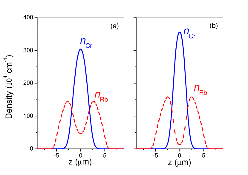
Figure 1: (Color online) Ground-state density profiles in the two-component dipolar BEC for $\varepsilon_{dd}=-0.3$ and different values of intercomponent scattering length: (A) $a_{12}=4$ nm; (B) $a_{12}=4.33$ nm (the critical point). In this figure and Figs. 2 and 3, the blue solid line represents the density profile of ⁵²Cr and the red dashed line is that of ⁸⁷Rb.

First, we assume $\varepsilon_{dd}=-0.3$ and calculate the density profiles of those two components for various $a_{12}$ using the coupled GP equations. For a relatively small value of the intercomponent scattering length $a_{12}$ (4 nm in Table 1), the two-component BEC does not separate [see Fig. 1 (A)]. Then we increase $a_{12}$ to the critical point (4.33 nm in Table 1), the phase separation of Cr and Rb atoms occurs and the density of Cr increases [see Fig. 1 (B)]. The dipoles in this case lie predominantly side by side, and the net dipolar interaction is attractive (repulsive) when $\varepsilon_{dd}<0$ $\left(\varepsilon_{dd}>0\right)$ Dell2008 . As a result, the effective interatomic interaction $U_{1}^{eff1}$ (containing the dipolar interaction and $s$-wave interaction) in Cr is less than the interatomic interaction $U_{2}$ in Rb, and both of them as well as the intercomponent interaction are repulsive (see Table 1). Then Cr pushes Rb out toward the edges of the trap, while the rubidium atoms also “squeeze” the chromium atoms, i.e., they act like a trap which enhances the trapping force on the chromium atoms and makes the peak density of Cr higher. In the one-dimensional case containing only $s$-wave scattering interactions, the criterion Eq. (10) works perfectly Nav . However, when we increase $\varepsilon_{dd}$ (as in Fig. 2 where $\varepsilon_{dd}=0.1$), the anticipated phase separation doesn’t occur at the critical point. Instead, the two components admix homogeneously [see Fig. 2 (A)]. By calculating the interactions’ strengths, we know that the two interatomic interactions and the intercomponent interaction have the same value (see Table 1); thus the two-component Bose gas behaves like a one-component Bose gas since all particles have, so to speak, the same hard-core diameter. As a result, all the atoms are in a homogeneous mixture. Increasing $a_{12}$ slightly beyond the critical value of the intercomponent scattering length, we find that the two components are repelled by each other. Since the intercomponent interaction is larger than the two interatomic interactions as shown in Table 1, none of the atoms stays at the center of the trap [see Fig. 2 (B)].

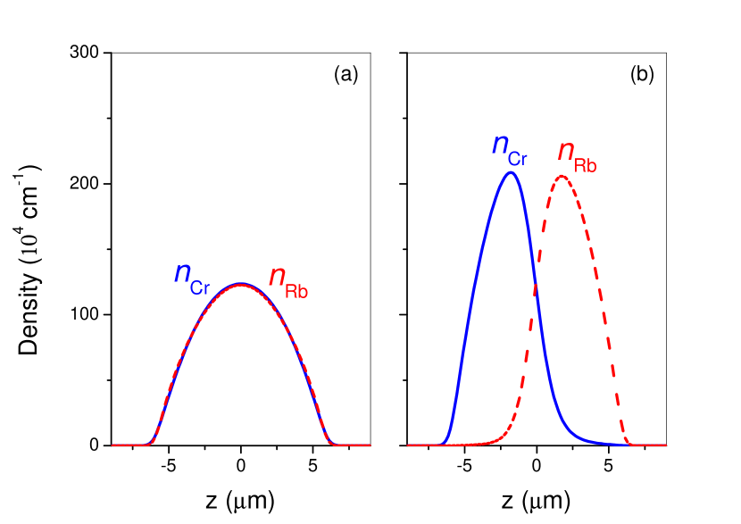
Figure 2: (Color online) Ground-state density profiles in the two-component dipolar BEC for $\varepsilon_{dd}=0.1$ and different values of the intercomponent scattering length: (A) $a_{12}=7.5$ nm (the critical point); (B) $a_{12}=7.6$ nm.

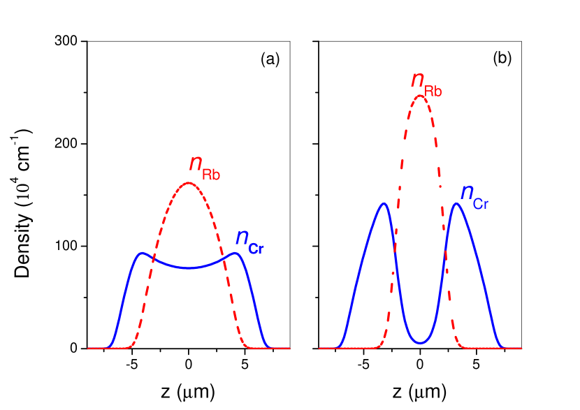
Figure 3: (Color online) Ground-state density profiles in the two-component dipolar BEC for $\varepsilon_{dd}=0.5$ and different values of the intercomponent scattering length: (A) $a_{12}=8$ nm; (B) $a_{12}=9.68$ nm (the critical point).

Increasing $\varepsilon_{dd}$ (as in the Fig. 3 where $\varepsilon_{dd}=0.5$), we find that the phase separation is different from that shown in Fig. 1. At the critical point, the rubidium atoms still occupy the center of the trap and their peak density becomes higher, while the chromium atoms are pushed out instead [see Fig. 3 (B)]. As we can see, this is because the effective interatomic interaction of the chromium BEC is now stronger than the interaction of the rubidium BEC (see Table 1), and the rubidium atoms get an extra trapping force from the chromium atoms. Based on this, we may control the component which we intend to move out of the trap center to some extent.

III Quasi-two-dimensional Regime (infinite cigar)

We now consider the two-component dipolar cigar-shaped BEC in a quasi-two-dimensional regime using a similar methodology to that for the pancake shape. If we neglect the axial trapping $\left(\omega_{iz}=0\right)$ and consider the BEC to be uniform along $z$, then Eq. (3) reduces to the contactlike form Dell2008 :

$$\Phi_{dd}=-U_{1}\varepsilon_{dd}n\left(\rho\right)=-U_{1}N_{1}\varepsilon_{dd}|\psi_{1}\left(\rho\right)|^{2}.$$ (11)

Then we can rewrite Eq. (5) and (6) as two dimensionless coupled differential equations:

$$H_{1} = -\frac{1}{2}\left(\frac{\partial^{2}}{\partial\rho^{2}}+\frac{1}{\rho}\frac{\partial}{\partial\rho}\right)+\frac{1}{2}\rho^{2}+4\pi N_{1}a_{1}(1-\varepsilon_{dd})\times$$ (12)

$$|\psi_{1}(\rho)|^{2}+\frac{1+a_{m}}{a_{m}}2\pi N_{2}a_{12}|\psi_{2}(\rho)|^{2}$$

$$H_{2} = -\frac{1}{2a_{m}}\left(\frac{\partial^{2}}{\partial\rho^{2}}+\frac{1}{\rho}\frac{\partial}{\partial\rho}\right)+\frac{1}{2}a_{m}a_{\omega}^{2}\rho^{2}+\frac{4\pi N_{2}a_{2}}{a_{m}}\times$$ (13)

$$|\psi_{2}\left(\rho\right)|^{2}+\frac{1+a_{m}}{a_{m}}2\pi N_{1}a_{12}|\psi_{1}\left(\rho\right)|^{2},$$

with units of length and energy and $a_{m}=m_{2}/m_{1}$ as in Sec. II, while $a_{\omega}=\omega_{2\rho}/\omega_{1\rho}$ is just different in form from that in Sec. II. Here, for simplicity and comparability, we assume that the values of these two $a_{\omega}$ are equivalent, i.e., $\omega_{2z}/\omega_{1z}=\omega_{2\rho}/\omega_{1\rho}$.

Using a similar methodology, we apply boundary conditions $\lim\limits_{\rho\rightarrow\infty}\psi_{i}\left(\rho\right)=0$ and $\frac{\partial}{\partial\rho}\psi_{i}(\rho)|_{\rho=0}=0$, and the finite-difference approximations finitediff

$$\frac{\partial^{2}\psi_{i}}{\partial\rho^{2}}=\frac{\psi_{i}^{l+1}-2\psi_{i}^{l}+\psi_{i}^{l-1}}{h^{2}},~{}\frac{\partial\psi_{i}}{\partial\rho}=\frac{\psi_{i}^{l+1}-\psi_{i}^{l-1}}{2h},$$

then we can write $H_{i}$ as a nonsymmetric tridiagonal matrix containing diagonal elements $\varsigma_{i}^{l}$, subdiagonal elements $\varpi_{i}^{l}$, and superdiagonal elements $\vartheta_{i}^{l}$ in $H_{i}$, where

$$\varsigma_{1}^{l}=2+2h^{2}\nu_{1}^{l},~{}\varsigma_{2}^{l}=\frac{2}{a_{m}}+2h^{2}\nu_{2}^{l},$$

$$\nu_{1}^{l} = \frac{1}{2}\rho_{l}^{2}+4\pi N_{1}a_{1}\left(1-\varepsilon_{dd}\right)|\psi_{1}^{l}|^{2}+\frac{1+a_{m}}{a_{m}}2\pi N_{2}a_{12}|\psi_{2}^{l}|^{2},$$

$$\nu_{2}^{l} = \frac{1}{2}\rho_{l}^{2}+\frac{4\pi N_{2}a_{2}}{a_{m}}|\psi_{2}^{l}|^{2}+\frac{1+a_{m}}{a_{m}}2\pi N_{1}a_{12}|\psi_{1}^{l}|^{2},$$

$$\varpi_{1}^{l}=-\left(1-\frac{h}{2\rho_{l}}\right),~{}\varpi_{2}^{l}=-\frac{1}{a_{m}}\left(1-\frac{h}{2\rho_{2}}\right),$$

$$\vartheta_{1}^{1}=-2,~{}\vartheta_{1}^{l\geq 2}=-\left(1+\frac{h}{2\rho_{l}}\right),$$

$$\vartheta_{2}^{1}=-\frac{2}{a_{m}},~{}\vartheta_{2}^{l\geq 2}=-\frac{1}{a_{m}}\left(1+\frac{h}{2\rho_{l}}\right),$$

$$\rho_{l}=\left(l-1\right)h,$$

with mesh length $h$ in the $\rho$ direction. By diagonalizing these two nonsymmetric tridiagonal matrices, we can get the ground state wave functions $\psi_{i}\left(\rho\right)$ and the density profiles of the dipolar BEC Pu . Here, the critical value $a_{12}^{c}$ is obtained by

$$a_{12}^{c}=\sqrt{\frac{4a_{1}\left(1-\varepsilon_{dd}\right)a_{2}a_{m}}{\left(1+a_{m}\right)^{2}}},$$ (14)

arising from $U_{1}^{eff2}U_{2}-U_{12}^{2}=0$ with $U_{1}^{eff2}=U_{1}\left(1-\varepsilon_{dd}\right)$.

We assume that $\omega_{1\rho}=2\pi\times 160$ Hz, the particle number is taken as $N_{1}=N_{2}=2000$, and $a_{m}a_{\omega}^{2}=1$ as well.

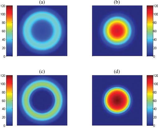
Figure 4: (Color online) Ground state density profiles in the two-component dipolar BEC for $\varepsilon_{dd}=-0.3$. The intercomponent scattering length $a_{12}=5.5$ nm in (A) and (B), while $a_{12}=7.81$ nm (the critical point) in (C) and (D). In this figure and Figs. 5 and 6, (A) and (C) represent the chromium atoms, while (B) and (D) represent the rubidium atoms. The numerical values of the units for density and length are respectively $1\times 10^{8}$ cm^-2 and $1$ $\mu$m in our calculations. The field of view for (A)-(D) is $10\times 10$ $\mu$m.

Table 2: Dimensionless values of interactions in quasi-two dimension

$\varepsilon_{dd}$	$U_{1}^{eff2}$ ($10^{-3}$)	$U_{12}$ ($10^{-3}$)	$U_{2}$ ($10^{-3}$)
-0.3	82	55 ($a_{12}=5.5$ nm) 78 ($a_{12}^{c}=7.81$ nm)	75
0.1	57	30 ($a_{12}=3$ nm) 65 ($a_{12}^{c}=6.5$ nm)	75
0.5	31	20 ($a_{12}=2$ nm) 49 ($a_{12}^{c}=4.84$ nm)	75

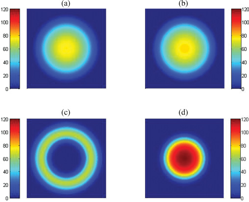
Figure 5: (Color online) Ground state density profiles in the two-component dipolar BEC for $\varepsilon_{dd}=0.1$. The intercomponent scattering length $a_{12}=3$ nm in (A) and (B), while $a_{12}=6.5$ nm, the critical point, in (C) and (D). The units are the same as in Fig. 4. The field of view for (A)-(D) is $10\times 10$ $\mu$m.

In this case, the dipoles are predominantly end to end, and the net dipolar interaction is repulsive (attractive) when $\varepsilon_{dd}<0$ $\left(\varepsilon_{dd}>0\right)$ Dell2008 . This is in contrast to the case in the quasi-one-dimensional regime. We then find that the chromium atoms are squeezed out when $\varepsilon_{dd}=-0.3$ at the critical point, and form a shell around the rubidium atoms which are situated at the center of the trap [see Fig. 4 (C) and (D)]. The critical point of $a_{12}$ in this case is not the same as in the quasi-one-dimensional regime, but higher. We believe the cause is that the effective interatomic interaction $U_{1}^{eff2}$ of Cr, which is repulsive, becomes stronger than in the former case (see Tables 1 and 2). We cannot observe a similar phase-separated state for $\varepsilon_{dd}=0.1$ as in Fig. 2 (B), other than in the quasi-one-dimensional regime. As shown in Fig. 5, the two components are mixed homogeneously at a small value of $a_{12}$ (3 nm in Table 2), and phase separation occurs at the critical point.

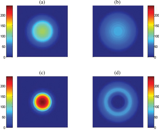
Figure 6: (Color online) Ground state density profiles in the two-component dipolar BEC for $\varepsilon_{dd}=0.5$. The intercomponent scattering length $a_{12}=2$ nm in (A) and (B), while $a_{12}=4.84$ nm, the critical point, in (C) and (D). The units are the same as in Fig. 4. The field of view for (A)-(D) is $10\times 10$ $\mu$m.

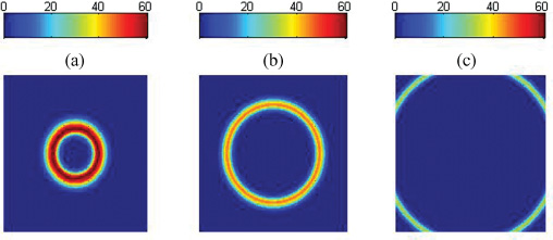
Figure 7: (Color online) Ground state density profiles of component 1 (Cr). $N_{1}=2\times 10^{3}$, $\varepsilon_{dd}=-0.3$, $a_{12}=a_{12}^{c}=7.81$. From (A) to (C), $N_{2}=2\times 10^{3}$, $N_{2}=2\times 10^{4}$, $N_{2}=2\times 10^{5}$, respectively. The units are the same as in Fig. 4. The field of view for (A)-(C) is $20\times 20$ $\mu$m.

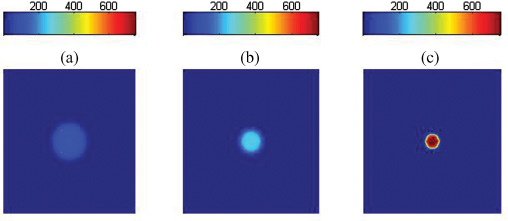
Figure 8: (Color online) Ground state density profiles of component 2 (Rb). $N_{2}=2\times 10^{3}$, $\varepsilon_{dd}=-0.3$, $a_{12}=a_{12}^{c}=7.81$. From (A) to (C), $N_{1}=2\times 10^{3}$, $N_{1}=2\times 10^{4}$, $N_{1}=2\times 10^{5}$, respectively. The units are the same as in Fig. 4. The field of view for (A)-(C) is $20\times 20$ $\mu$m.

On increasing $\varepsilon_{dd}$ to 0.5, we find that the attractive strength of the dipolar interaction becomes very large, and the chromium atoms begin to occupy the center of the trap, while the rubidium atoms form a shell around chromium (see Fig. 6). The phase-separated states for the same $\varepsilon_{dd}$ are totally different between the quasi-one- and quasi-two-dimensional regimes. The interactions are known to be the predominant factors which can affect the ground-state density profile of a BEC, so different properties of the dipolar interaction can make a difference to the phase separations between the two regimes. For the same value of $\varepsilon_{dd}$, the repulsion or attraction of the net dipolar interaction is opposite in the two regimes, so the effective interatomic interaction of Cr is totally different between the two regimes (compare $U_{1}^{eff2}$ of Table 2 with $U_{1}^{eff1}$ of Table 1). If $\varepsilon_{dd}$ is negative, the repulsion of the effective interatomic interaction in the quasi-two-dimensional regime is much stronger than in the quasi-one-dimensional regime (see Tables 1 and 2), so the rubidium atoms are held at the center of the trap while the chromium atoms are forced to form a shell around the center at the critical point of phase separation. The situation for a relatively large positive $\varepsilon_{dd}$ is the opposite.

In addition to the strength of the interactions, the density profiles also depend on the particle numbers $N_{1}$ and $N_{2}$ Pu . Thus we do some calculations where we hold constant the number of one component’s atoms and change the other in the quasi-two-dimensional regime. Clearly, the number of atoms plays a key role in the phase separation of a two-component BEC. In the case of $\varepsilon_{dd}=-0.3$, Cr forms a shell around Rb. When the number of Cr atoms is fixed, they are squeezed further out as the number of Rb atoms increases (See Fig. 7). If we fix the number of Rb atoms instead, one can see that the rubidium atoms are compressed further as the number of Cr increases (See Fig. 8). Finally, we would like to mention that the situation of the quasi-one-dimensional regime is similar to this case herein.

IV Conclusion

In the present work, we have analyzed the phase separation of a two-component dipolar BEC in the quasi-one- and quasi-two-dimensional regimes, as a natural parameter of the system (the intercomponent interaction strength) was varied. Our analysis was presented for the case of a two-component Bose-Einstein condensate trapped in a harmonic-oscillator potential.

We reduced the long-range dipole-dipole interaction to a contactlike form, when a dipole moment is aligned along the $z$ direction, and then used a numerical method to solve two coupled nonlinear Gross-Pitaevskii equations in the low-dimensional regime. We were able to elucidate the phase separation condition for the intercomponent coupling parameter as the dimensionless dipolar interaction strength parameter $\varepsilon_{dd}$ was varied.

Both repulsive and attractive dipolar interactions have been taken into consideration. Among all the phase-separated states, $\varepsilon_{dd}$ plays a significant role. By modulation of its strength, the two components might alternately stay in or be forced to be outside the center of the trap. In addition to the interactions, we considered the dependence of the density profiles on the number of atoms as well.

We also described the differences between the quasi-one- and quasi-two-dimensional regimes in detail. Due to the anisotropic property of the dipole-dipole interaction, phase separation in the axial direction differs from that in the radial direction.

A natural extension of this work is to try to generalize the ideas presented herein to higher dimensions or larger number of components (i.e., spinors). Especially in the former case, more complicated pattern formations on the interface, such as Rosensweig hexagonal peaks and a labyrinthine pattern, have been observed Ueda2009 . Such studies are presently in progress and will be presented in future work.

V Acknowledgement

J. B. L. is grateful to Yue Yu for his encouragement. We would also like to thank Su Yi for comments. This work is supported by the Natural Science Foundation of Jiangsu Province (NSFJS, Grant No. BK2010499) and MOE of China (Grant No. 20070287062).

References

- (1) S. Giovanazzi, A. Görlitz, and T. Pfau, Phys. Rev. Lett. 89, 130401 (2002).
- (2) A. Griesmaier, J. Werner, S. Hensler, J. Stuhler, T. Pfau, Phys. Rev. Lett. 94, 160401 (2005); J. Stuhler, A. Griesmaier, T. Koch, M. Fattori, T. Pfau, S. Giovanazzi, P. Pedri, L. Santos, ibid. 95, 150406 (2005); M. Fattori, T. Koch, S. Goetz, A. Griesmaier, S. Hensler, J. Stuhler, T. Pfau, Nature Phys. 2, 765 (2006).
- (3) A. Griesmaier, J. Stuhler, T. Koch, M. Fattori, T. Pfau, S. Giovanazzi, Phys. Rev. Lett. 97, 250402 (2006).
- (4) T. Lahaye, T. Koch, B. Frölich, M. Fattori, J. Metz, A. Griesmaier, S. Giovanazzi, T. Pfau, Nature 448, 672 (2007). T. Koch, T. Lahaye, J. Metz, B. Frölich, A. Griesmaier, T. Pfau, Nature Phys. 4, 218 (2008); T. Lahaye, J. Metz, B. Frölich, T. Koch, M. Meister, A. Griesmaier, T. Pfau, H. Saito, Y. Kawaguchi, M. Ueda, Phys. Rev. Lett. 101, 080401 (2008).
- (5) K. Góral, K. Rza̧żewski, and T. Pfau, Phys. Rev. A 61, 051601 (2000). L. Santos, G.V. Shlyapnikov, P. Zoller, and M. Lewenstein, Phys. Rev. Lett. 85, 1791 (2000).
- (6) S. Giovanazzi, D. O’Dell, and G. Kurizki, Phys. Rev. Lett. 88, 130402 (2002). K. Góral, L. Santos, and M. Lewenstein, ibid 88, 170406 (2002).
- (7) S. Yi and L. You, Phys. Rev. A 61, 041604(R) (2000).
- (8) S. Yi and L. You, Phys. Rev. A 63, 053607 (2001); S. Yi and L. You, ibid. 66, 013607 (2002).
- (9) K. Góral and L. Santos, Phys. Rev. A 66, 023613 (2002).
- (10) T. Lahaye, C. Menotti, L. Santos, M. Lewenstein, and T. Pfau, Rep. Prog. Phys. 72, 126401 (2009).
- (11) Tin-Lun Ho and V. B. Shenoy, Phys. Rev. Lett. 77, 3276 (1996); E. Timmermans, ibid. 81, 5718 (1998).
- (12) H. Pu and N. P. Bigelow, Phys. Rev. Lett. 80, 1130 (1998).
- (13) C.J. Myatt, E.A. Burt, R.W. Ghrist, E.A. Cornell, and C.E. Wieman, Phys. Rev. Lett. 78, 586 (1997); D.M. Stamper-Kurn, M.R. Andrews, A.P. Chikkatur, S. Inouye, H.-J. Miesner, J. Stenger, and W. Ketterle, Phys. Rev. Lett. 80, 2027 (1998); D.S. Hall, M.R. Matthews, J.R. Ensher, C.E. Wieman, and E.A. Cornell, Phys. Rev. Lett. 81, 1539 (1998).
- (14) V. Schweikhard, I. Coddington, P. Engels, S. Tung, and E.A. Cornell, Phys. Rev. Lett. 93, 210403 (2004); K.M. Mertes, J.W. Merrill, R. Carretero-González, D.J. Frantzeskakis, P.G. Kevrekidis, and D.S. Hall, ibid. 99, 190402 (2007); S.B. Papp, J.M. Pino, and C.E. Wieman, ibid. 101, 040402 (2008).
- (15) Hiroki Saito, Yuki Kawaguchi, and Masahito Ueda, Phys. Rev. Lett. 102, 230403 (2009).
- (16) Goran Gligorić, Aleksandra Maluckov, Milutin Stepić, Ljupčo Hadžievski, and Boris A. Malomed, Phys. Rev. A 82, 033624 (2010).
- (17) C. J. Pethick and H. Smith, Bose-Einstein Condensation in Dilute Gases, 2nd ed. (Cambridge University Press, Cambridge, U.K., 2008).
- (18) D. O’Dell, S. Giovanazzi, and C. Eberlein, Phys. Rev. Lett. 92, 250401 (2004); C. Eberlein, S. Giovanazzi, and D. O’Dell, Phys. Rev. A 71, 033618 (2005); D. O’Dell and C. Eberlein, ibid. 75, 013604 (2007).
- (19) N.G. Parker and D. O’Dell, Phys. Rev. A 78, 041601(R) (2008).
- (20) J.W. Thomas, Numerical Partial Differential Equations: Finite Difference Methods, Springer, 1995.
- (21) P. Ao and S. T. Chui, Phys. Rev. A 58, 4836 (1998).
- (22) M. Theis, G. Thalhammer, K. Winkler, M. Hellwig, G. Ruff, R. Grimm, and J. H. Denschlag, Phys. Rev. Lett. 93, 123001 (2004).
- (23) R. Navarro et al., Phys. Rev. A 80, 023613 (2009); S. Gautam and D. Angom, J. Phys. B: At. Mol. Opt. Phys. 44 025302 (2011).