Expanding the thermodynamical potential and the analysis of the possible phase diagram of deconfinement in FL model

Abstract

The deconfinement phase transition is studied in the FL model at finite temperature and chemical potential. At MFT approximation, the phase transition can only be the first order in the whole $\mu-T$ phase plane. By a Landau expansion we further study the phase transition order and the possible phase diagram of deconfinement. We discuss the possibilities of second order phase transitions in FL model. By our analysis the cubic term in the Landau expansion could be cancelled by the high order fluctuations. By an ansatz of the Landau parameters, we obtain the possible phase diagram with both first and second order phase transition including the tricritical point which is similar to that of the chiral phase transition.

I Introduction

It is generally believed that at sufficiently high temperatures and densities there is a QCD phase transition from normal nuclear matter to QGP ref1 ; ref2 . Theoretically there are two kinds of phase transitions associated with different symmetries for two opposite quark mass limit. For $N_{f}=2+1$ massless quark flavors, the QCD lagrangian posses a chiral symmetry $SU(N_{f})_{R}\times SU(N_{f})_{L}$, which is associated with the chiral phase transition. In the heavy quark limit, QCD reduces to a pure $SU(N_{c})$ gauge theory which is invariant under a global $Z(N_{c})$ center symmetry. This symmetry is associated with the deconfinement phase transition. The orders of these phase transitions have been studied extensively ref3 ; ref4 ; ref5 and still remained to be an interesting problem ref6a ; ref6b ; ref6c ; ref6d . For chiral phase transition at finite temperature in the chiral limit, the quark-antiquark condensate $\langle\bar{q}_{R}q_{L}\rangle$ serves as a good order parameter. The order of the phase transition depends on the quark flavors. For $N_{f}=3$ massless quark flavors, it is a first order phase transition. For $N_{f}=2$ massless quark flavors, it is a second order phase transition. At finite densities, the chiral phase transition have been studied by many effective models ref7 ; ref8 ; ref9 . It is generally regarded that at high densities it is a first order phase transition. In the $\mu-T$ phase diagram, from first chiral phase transition to second order phase transition there exists a tri-critical point(TCP). For deconfinement phase transition, it has not a good order parameter except for infinite quark mass limit, at which the Polyakov loop severs as an order parameter ref10 ; ref11 . In recent studies the Polyakov loop has been combined into the chiral models,such as Nambu-Jona-Lasinio model ref12 ; ref13 and linear sigma model ref14 ; ref15 ; ref16 , which allows to investigate the deconfinement phase transition within the chiral models. Though the Polyakov loop is not a good order parameter, it still serves as an indicator of a rapid crossover towards deconfinement. As we know in the Landau theory, for the study of the phase transition and the transition order, one should find a good order parameter. Once it is identified, the thermodynamic functions could be expanded over this order parameter and the transition order could be well studied. For the deconfinement phase transition, besides the Polyakov loop, one can also search for other proper order parameters in the effective field models. In the earlier studies of deconfinement, the bag models had been often used to investigate the confinement mechanics and the thermodynamics of deconfinement phase transition. In this paper we wish to use the effective bag model to study the deconfinement phase transition and mainly focus on the study of the transition order and the possible phase diagram of the deconfinement, especially the possible influence on the phase diagram by the fluctuations.

The model we used here is Friedberg-Lee(FL) soliton bag model. The FL model has been widely discussed in past decays ref17 ; ref18 ; ref19 . It has been very successful in describing phenomenologically the static properties of hadrons and their behaviors at low energy. The model consists of quark fields interacting with a phenomenological scalar field $\sigma$. The $\sigma$ field is introduced to describe the complicated nonperturbative features of QCD vacuum. It naturally gives a color confinement mechanism in QCD theory. The model has been also extended to finite temperatures and densities to study deconfinement phase transition ref20 ; ref21 ; ref22 ; ref23 ; ref24 . Here we will try to identify the proper order parameter in this model and make an analysis of deconfinement phase transition.

The organization of this paper is as follows: in section 2 we give a brief introduction of the FL model. The thermodynamic potential is derived and deconfinement phase transition is discussed at finite temperatures and densities at mean field theory (MFT) approximation. In section 3, we make a Landau expansion of the thermodynamic potential. In this way the transition order is studied by analyzing the Landau coefficients. By an ansatz of Landau coefficients we discuss the possible phase diagram of deconfinement in FL model. The last section is the summary.

II The thermodynamic potential and deconfinement phase transition in FL model at MFT

We start from the Lagrangian of the FL model,

$${\cal L}=\bar{\psi}(i\gamma_{\mu}\partial^{\mu}-g\sigma)\psi+\frac{1}{2}(\partial_{\mu}\sigma)(\partial^{\mu}\sigma)-U(\sigma),$$ (1)

where

$$U(\sigma)=\frac{1}{2!}a\sigma^{2}+\frac{1}{3!}b\sigma^{3}+\frac{1}{4!}c\sigma^{4}+B.$$ (2)

$\psi$ represents the quark field, and $\sigma$ denotes the phenomenological scalar field. $a,b,c,g$ and $B$ are the constants which are generally fitted in with producing the properties of hadrons appropriately at zero temperature. We shift the $\sigma$ field as $\sigma\rightarrow\bar{\sigma}+\sigma^{\prime}$ where $\bar{\sigma}$ and $\sigma^{\prime}$ are the vacuum expectation value and the fluctuation of the $\sigma$ field respectively. Then the lagrangian becomes

$${\cal L}_{eff}=\bar{\psi}(i\gamma_{\mu}\partial^{\mu}-m_{q})\psi+\frac{1}{2}(\partial_{\mu}\sigma^{\prime})(\partial^{\mu}\sigma^{\prime})-\frac{1}{2}m_{\sigma}^{2}\sigma^{\prime 2}-U(\bar{\sigma}),$$ (3)

where

$$U(\bar{\sigma})=\frac{1}{2!}a\bar{\sigma}^{2}+\frac{1}{3!}b\bar{\sigma}^{3}+\frac{1}{4!}c\bar{\sigma}^{4}+B.$$ (4)

$m_{q}=g\bar{\sigma}$ and $m_{\sigma}^{2}=a+b\bar{\sigma}+\frac{1}{2}c\bar{\sigma}^{2}$ are the effective masses of the quark and $\sigma$ fields respectively. The interactions associated with the fluctuation $\sigma^{\prime}$, such as $\sigma^{\prime 3}$, $\sigma^{\prime 4}$ and $\bar{\psi}\sigma^{\prime}\psi$, are neglected in MFT approximation.

According to finite temperature field theory, the partition function is

$$Z=\int[d\bar{\psi}][d\psi][d\sigma^{\prime}]\exp\left[\int_{0}^{\beta}d\tau\int d^{3}{\bf x}({\cal L}_{eff}+\mu\psi^{{\dagger}}\psi)\right].$$ (5)

where $\mu$ is chemical potential of quarks. Completing the integration in partition function $Z$, together with the thermodynamic potential: $\Omega=-TlnZ$, at mean field level, we could obtain

$$\Omega=U(\bar{\sigma})+\frac{1}{\beta}\int\frac{d^{3}\bf p}{(2\pi)^{3}}\ln(1-e^{-\beta E_{\sigma}})-\frac{\gamma}{\beta}\int\frac{d^{3}\bf p}{(2\pi)^{3}}\left[\ln(1+e^{-\beta(E_{q}-\mu)})+\ln(1+e^{-\beta(E_{q}+\mu)})\right],$$ (6)

where $\beta$ is the inverse of the temperature $T$ and $\gamma$ is a degenerate factor that $\gamma=2(spin)\times 2(flavor)\times 3(color)$. In addition, $E_{\sigma}=\sqrt{\vec{p}^{2}+m_{\sigma}^{2}}$ and $E_{q}=\sqrt{\vec{p}^{2}+m_{q}^{2}}$.

Figure 1: The thermodynamical potentials for different temperatures and zero chemical potential: $T_{0}=0MeV$, $T_{1}=100MeV$, $T_{c}=121MeV$ and $T_{2}=130MeV$.

Figure 2: The thermodynamical potentials for different chemical potentials and fixed temperature at $T=50MeV$: $\mu_{1}=100MeV$, $\mu_{2}=200MeV$, $\mu_{c}=255MeV$, and $\mu_{3}=300MeV$.

In our calculation, the parameters are chosen to be $a=17.7fm^{-2},b=-1457.4fm^{-1},c=20000,g=12.16$. The effective mass of $\sigma$ field is fixed at $m_{\sigma}=550MeV$ ref22 . Then one could plot $\Omega$ versus $\bar{\sigma}$ for different $T$ as shown in Fig.1. At zero temperature, where $\Omega=U(\bar{\sigma})$, there are two minima of the thermodynamic potential: one corresponds to the perturbative vacuum at $\bar{\sigma}=0$, another corresponds to the physical vacuum at $\bar{\sigma}=\sigma_{v}$. The system is stabled at the physical vacuum at $\bar{\sigma}=\sigma_{v}$. It is well known that at this time the quarks are confined in a soliton bag, and the system is in a hadronic phase. With temperature increased, the physical vacuum $\bar{\sigma}=\sigma_{v}$ is lifted up, while the quarks has been still confined until the two vacuums degenerate. At this time the deconfinement phase transition occurs, and the phase transition temperature is $T=T_{c}$. After that, the system is stabled at the perturbative vacuum $\bar{\sigma}=0$, where the quarks are deconfined and the system is in a deconfined phase. This is a first order phase transition.

One can also plot the $\Omega$ versus $\bar{\sigma}$ at different $\mu$ for $T=50MeV$ as shown in Fig.2. The deconfinement phase transition takes place at $\mu=\mu_{c}$ where the two vacuums degenerate. The analysis of deconfinement phase transition at finite chemical potential is similar to that at finite temperature.

Figure 3: The $\mu-T$ phase diagram of deconfinement at MFT in the FL model.

One can obtain the $\mu-T$ phase diagram as shown in Fig.3. In the whole $\mu-T$ phase plane, the transition is first order.

III A Landau expansion and the possible phase diagram of deconfinement phase transition

In above discussion, we know at MFT approximation in FL model the deconfinement phase transition is first order. One can plot the $\bar{\sigma}$ as a function of $T$, as shown in Fig.4. It could be seen that at $T=T_{c}$, $\bar{\sigma}$ jumps from nonzero value $\bar{\sigma}=\sigma_{v}$ to zero value $\bar{\sigma}=0$. In confined phase $\bar{\sigma}\neq 0$; in deconfined phase $\bar{\sigma}=0$. Here $\bar{\sigma}$ could be viewed as an order parameter of deconfinement phase transition in FL model, so we can do a Landau expansion of $\Omega$ based on $\bar{\sigma}$ and make a thorough investigation of the phase transition order.

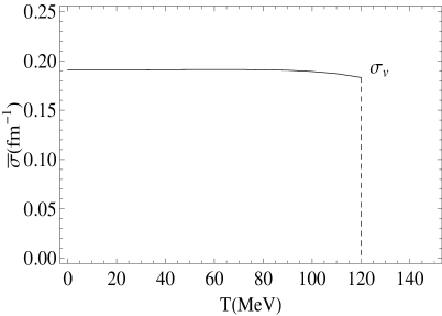
Figure 4: $\bar{\sigma}$ as a function of $T$ at zero chemical potential in the FL model.

At the MFT approximation, from equation (6) the thermodynamic potential could be power expanded by $\bar{\sigma}$ with $\bar{\sigma}^{2}$, $\bar{\sigma}^{3}$ and $\bar{\sigma}^{4}$. However, the analytical forms of the coefficients of the expansion are difficult to be obtained. Here we will write down the effective form of the expansion as

$$\Omega=\frac{1}{2}A(T,\mu)\bar{\sigma}^{2}+\frac{1}{3!}B(T,\mu)\bar{\sigma}^{3}+\frac{1}{4!}C(T,\mu)\bar{\sigma}^{4},$$ (7)

where $A(T,\mu)$, $B(T,\mu)$ and $C(T,\mu)$ are the effective parameters which could be determined by a numerical fitting process. That means at certain $T$ and $\mu$ from the configuration of the $\Omega$ versus $\bar{\sigma}$ one could fit the curve by the $\bar{\sigma}^{2}$, $\bar{\sigma}^{3}$ and $\bar{\sigma}^{4}$ to obtain the values of $A(T,\mu)$, $B(T,\mu)$ and $C(T,\mu)$. By the equation (7), from Landau theory, it is clear that the cubic term $\bar{\sigma}^{3}$ plays crucial role in determination of the transition order. At MFT approximation, the fitting results indicate that $B(T,\mu)$, as a negative value, will keep decreasing with temperature and/or chemical potential increasing. That means this term will never be zero, therefore the transition order of deconfinement at MFT approximation can only be first order.

Now we suppose equation (7) is the general form of expansion of thermodynamical potential by order parameter $\bar{\sigma}$ in FL model. And we regard the corrections coming from the fluctuations will effectively modify the parameters $A(T,\mu)$, $B(T,\mu)$ and $C(T,\mu)$. In principle they could be calculated by self-consistently resumming the higher order loop diagrams led by the fluctuations of $\sigma^{\prime}$. However it is very difficult to evaluate these corrections in this way. In the following we will treat the coefficients $A(T,\mu)$, $B(T,\mu)$ and $C(T,\mu)$ as the free parameters and make a general study of the phase transition order on the FL model by Landau theory.

Figure 5: Phase diagram of deconfinement on the $A-B$ plane in the FL model.

In Landau theory, one can make a derivative of the thermodynamic potential to $\bar{\sigma}$ as

$$\frac{d\Omega}{d\bar{\sigma}}=A(T,\mu)\bar{\sigma}+\frac{1}{2}B(T,\mu)\bar{\sigma}^{2}+\frac{1}{3!}C(T,\mu)\bar{\sigma}^{3}=0.$$ (8)

One can obtain three solutions:

$$\bar{\sigma}_{1}=0,\ \ \ \ \ \bar{\sigma}_{2,3}=\frac{-3B\pm\sqrt{9B^{2}-24AC}}{2C}.$$ (9)

In our case, we assume $C>0$ which guarantees that the vacuums are the minima. When $3B^{2}\leq 8AC$, there is only one minimum at $\bar{\sigma}=0$. When $3B^{2}>8AC$, there are two minima. They correspond to the perturbative vacuum at $\bar{\sigma}=0$ and the physical vacuum at $\bar{\sigma}=\sigma_{v}$. When the two minima degenerate, one can obtain the condition that: $B^{2}=3AC$, at which the deconfinement phase transition takes place. Thus one can draw the critical line of the deconfinement phase transition in the plane of $B$ versus $A$ as shown in Fig.5. The phase plane has been divided into two parts: the left area beside the line in the plane represents the confined phase, while the right area the deconfined phase. By analyzing the variation of the vacuum, one can obtain that the deconfinement phase transition can be either first or second order. If the system goes across the critical line at $B\neq 0$, the transition is first order. If the system goes across the line at $B=0$, the transition is second order.

Figure 6: The thermodynamical potentials for different temperatures and zero chemical potential. The temperatures are $100MeV,150MeV,180MeV$ and $200MeV$ from bottom to top.

From above discussion by Landau theory, we know there may be a second order phase transition in FL model, while at MFT level, the deconfinement phase transition can only be first order. But if we consider fluctuations beyond MFT, there are maybe additional terms which cancel the cubic $\bar{\sigma}^{3}$ term. The second order phase transition may be possible. That means the parameter $B(T,\mu)$ will go to zero before the transition takes place. The system will evolve from left area to right area across the critical line by the axis origin in the Fig.5. In our former calculation at MFT, the fluctuations of $\sigma^{\prime}$ in the Lagrangian have been neglected. These terms are possibly important in the cancellation of the cubic term. However, it is very difficult to calculate the thermodynamic potential including these fluctuations from the Lagrangian in FL model. In the following, we will make an ansatz based on the form of the Landau expansion of the thermodynamic potential to mimic the deconfinement phase transition which have both first and second order phase transition.

Figure 7: The thermodynamical potentials for different chemical potentials and zero temperature. The chemical potentials are $350MeV,392MeV,420MeV$ and $470MeV$ from bottom to top.

We can devise a possible variation pattern of $A(T,\mu)$, $B(T,\mu)$ and $C(T,\mu)$. We suppose at finite temperature and zero chemical potential, the absolute value of $B(T,\mu)$ keeps decreasing and tends to zero with temperature increasing, while $A(T,\mu)$ first decreases to a negative value and then increases with temperature increasing. $C(T,\mu)$ keeps positive in all the cases. By this kind of variation, from Fig.5, one could see that the system will evolve from the confined phase to the deconfined phase across the axis origin, and the transition will be second order. Thus we make the following ansatz of $A(T,\mu)$, $B(T,\mu)$ and $C(T,\mu)$ as

$$A(T,\mu) = a\left[(T-T_{c})(k_{1}T-\frac{1}{T_{c}})+\lambda_{1}\mu^{2}\right],$$ (10)

$$B(T,\mu) = bExp\left[-k_{2}\left(\frac{T+T_{c}}{T_{c}}\right)^{6}+k_{2}+\lambda_{2}\mu\right],$$ (11)

$$C(T,\mu) = c,$$ (12)

where $a,b$ and $c$ are the parameters of the FL model which have been already given in section II. $k_{1}=4fm^{2},k_{2}=0.15,\lambda_{1}=0.5fm^{2}$ and $\lambda_{2}=0.1fm$ are the effective parameters of the ansatz. $T_{c}$ is the critical temperature of the transition at zero chemical potential which could be seen in later analysis. It also serves as a temperature scaling factor which value can be taken as $T_{c}=180MeV$. When $T=\mu=0$, it is clear that $A(0,0)=a$, $B(0,0)=b$ and $C(0,0)=c$. One should notice that in our ansatz with the temperature increasing the parameter $B(T,\mu)$ will be infinitely close to zero but not zero. However when the second order phase transition takes place, the absolute value of $B(T,\mu)$ will be sufficiently small. At zero chemical potential, from equation (10), one could see at $T=T_{c}$, $A(T_{c},0)=0$. At the same time $B(T_{c},0)\approx 0$. Thus the deconfinement phase transition at zero chemical potential and finite temperature takes place at $T=T_{c}=180MeV$ and the transition order is second order. At zero temperature, from equation (11), one could see that $B(0,\mu)$ will never be zero with chemical potential increasing, which means the transition will be first order at zero temperature and finite chemical potential.

We can also evaluate the thermodynamic potential for different chemical potentials and temperatures. At finite temperature and zero chemical potential, the thermodynamic potential as a function of $\bar{\sigma}$ is plotted in Fig.6. It is clear that the phase transition is second order. At zero temperature and finite chemical potential, it could be seen from Fig.7 that the transition is first order. The deconfinement phase transition could be presented in a $\mu-T$ phase diagram as shown in Fig.8. From first order phase transition to second order phase transition there exists a TCP. The phase diagram is qualitatively consistent with that of the chiral phase transition. However, how to obtain the credible phase diagram of deconfinement through the direct calculations including the fluctuations from the Lagrangian of the FL model deserves a further investigation.

Figure 8: $\mu-T$ phase diagram of deconfinement with TCP in the FL model.

IV summary

In this paper we have discussed the possible phase diagram of deconfinement in FL model. By the calculation only in the MFT approximation and without the fluctuations, the deconfinement phase transition can only be first order at finite temperature and chemical potential. By the Landau expansion of the thermodynamic potential and the analysis through Landau theory, we show that the deconfinement phase transition can also be second order, which will not appear in the MFT approximation but will possibly appear when nonlinear fluctuations are considered. Thinking of the difficulties in calculating the fluctuations, we have not done the calculation here but made the ansatz that the Landau coefficients are certain functions of temperature and chemical potential. By this ansatz we obtain the possible $\mu-T$ phase diagram of deconfinement in FL model which is similar to that of the chiral phase transition. That means the deconfinement phase transition is first order at low temperature and high chemical potential while second order at high temperature and low chemical potential. From first order to second order phase transition there exists a TCP.

- (1) M. Gyulassy and L. McLerran, Nucl. Phys. A750, (2005) 30.
- (2) J.I. Kapusta, J. Phys. G34 (2007) S295-304.
- (3) B. Svetisky and L.G. Yaffe, Nucl. Phys. B210 (1982) 423.
- (4) R.D. Pisarski and F. Wilczek, Phys.Rev. D29 (1984) 338.
- (5) E. Shuryak and T. Schaefer, Phys. Rev. Lett. 75 (1995) 1707.
- (6) M. Alford, K. Rajagopal, and F. Wilczek, Phys. Lett. B 422 (1998) 247; J. Berges and K. Rajagopal, Nucl. Phys. B 538 (1999) 215.
- (7) L. McLerran and R.D. Pisarski, Nucl. Phys. A796 (2007) 83-100; L. McLerran, K. Redlich and C. Sasaki, Nucl. Phys. A824 (2009) 86-100.
- (8) K. Fukushima, Phys. Rev. D68 (2003) 045004; Y. Nishida, K. Fukushima and T. Hatsuda, Phys. Rept. 398 (2004) 281-300.
- (9) F. Karsch, Lect. Notes Phys. 583 (2002) 209-249.
- (10) O. Scavenius, A. Mocsy, I.N. Mishustin and D.H. Rischke, Phys. Rev. C64 (2001) 045202.
- (11) M. Stephanov, K. Rajagopal and E. Shuryak, Phys.Rev.Lett. 81 (1998) 4816-4819.
- (12) M. Alford, K. Rajagopal and F. Wilczek, Phys.Lett. B422 (1998) 247-256.
- (13) A.M. Polyakov, Phys. Lett. B72 (1978) 477.
- (14) B. Svetitsky, Phys. Rept. 132 (1986) 1.
- (15) K. Fukushima, Phys. Lett. B591 (2004) 277.
- (16) S. Roessner, C. Ratti and W. Weise, Phys. Rev. D75 (2007) 034007.
- (17) B.J. Schaefer, J.M. Pawlowski and J. Wambach, Phys. Rev. D76 (2007) 074023.
- (18) T. Kahara and K. Tuominen, Phys. Rev. D78 (2008) 034015.
- (19) H. Mao, J. Jin and M. Huang, J. Phys. G37 (2010) 035001.
- (20) R. Friedberg and T.D. Lee, Phys. Rev. D15, (1977) 1694; D16, (1977) 1096; D18, (1978) 2623.
- (21) R. Goldflam and L. Wilets, Phys. Rev. D25 (1982) 1951.
- (22) M.C. Birse, Prog. Part. Nucl. Phys. 25 (1990) 1.
- (23) H. Reinhardt, B.V. Dang and H. Schulz, Phys. Lett. B159 (1985) 161.
- (24) M. Li, M.C. Birse and L. Wilets, J.Phys. G13 (1987) 1.
- (25) E.K. Wang, J.R. Li and L.S. Liu, Phys. Rev. D41 (1990) 2288; S. Gao, E.K. Wang and J.R. Li, Phys. Rev. D46 (1992) 3211; S.H. Deng and J.R. Li, Phys.Lett. B302 (1993) 279.
- (26) H. Mao, R.K. Su and W.Q. Zhao, Phys. Rev. C74 (2006) 055204; H. Mao, M.J. Yao and W.Q. Zhao, Phys. Rev. C77 (2008) 065205.
- (27) S. Shu and J.R. Li, Phys. Rev. C82 (2010) 045203.