Finite-Size Scaling Analysis of the Distributions of Pseudo-Critical Temperatures in Spin Glasses

Abstract

Using the results of large scale numerical simulations we study the probability distribution of the pseudo critical temperature for the three dimensional Edwards-Anderson Ising spin glass and for the fully connected Sherrington-Kirkpatrick model. We find that the behaviour of our data is nicely described by straightforward finite-size scaling relations.

I Introduction

A proper phase transition takes place only in the idealised limit of an infinite number of interacting degrees of freedom. Although this limit is never realised in the laboratory (let alone in numerical simulations), everyday experience suggests that macroscopic samples are infinite for all practical purposes. Spin glasses mydosh:93 ; fisher:93 are an exception. The problem lies in their sluggish dynamics at the critical temperature and below. The system remains for very long times, or forever, out of equilibrium. In fact, letting the system relax for about one hour, the spatial size of the glassy magnetic domains is (at most) of the order of one hundred lattice spacings ORBACH .

It has become clear lately that, in order to interpret experimental data in spin glasses, the relevant equilibrium properties are those of systems of size similar to that of the experimentally achievable coherence length janus:10 ; janus:10b . Phase transitions on finite systems are actually crossover phenomena describable through the well known theory of finite size scaling (see e.g. amit:05 ). However, a conspicuous feature of disordered systems (and most notably, of spin glasses) is to undergo strong sample-to-sample fluctuations in many thermodynamic properties. It is thus natural to ask questions about the probability distribution, induced by the disorder, of the various physical quantities. Typically the size of these fluctuations decreases when enlarging the size of the equilibrated system; if we wish to have hints about their possible relevance in experimental systems, it is important to know the rate at which fluctuations decrease with system size. This is particularly important if we are to study dynamical heterogeneities BIROLI-BOUCHAUD in spin glasses janus:10b . In particular, a relevant but elusive physical quantity (potentially relevant to analyse dynamical effects close to the phase transition) is the finite-system pseudo-critical temperature. Our scope here is to characterise its statistical properties in spin glasses.

This problem has been extensively studied and is well understood for finite-size weakly bond-disordered spin models, below the upper critical dimension $d_{\text{up}}$. For a system of size $N=L^{d}$ and a disorder sample $J$, one can define a pseudo-critical temperature ${T_{\mathrm{c}}^{J}(L)}$ as the location of the maximum of a relevant susceptibility: this definition is clearly non unique, but all sensible definitions lead to the same scaling behaviour as $N\to\infty$. According to the Harris criterion Harris , a major role AH ; Paz1 ; Domany ; AHW ; Paz2 is played here by the value of the thermal critical exponent of the pure system, $\nu_{P}$. If $\nu_{P}>2/d$ the disorder is irrelevant, the value of $\nu$ is not modified by the disorder (i.e. $\nu=\nu_{P}$), and the width ${\Delta T_{\mathrm{c}}(L)}$ of the probability distribution of the pseudo-critical temperature, defined as ${\Delta T_{\mathrm{c}}(L)}^{2}\equiv E({T_{\mathrm{c}}^{J}(L)}^{2})-E({T_{\mathrm{c}}^{J}(L)})^{2}$, where $E(\cdots)$ denotes the disorder average, behaves as ${\Delta T_{\mathrm{c}}(L)}\propto 1/L^{d/2}$ as expected naively Domany95 . In such a situation in the infinite volume limit the (disorder induced) fluctuations of ${T_{\mathrm{c}}^{J}(L)}$ are negligible with respect to the width of the critical region and to the finite-size shift of $T_{\mathrm{c}}$, that both behave like $L^{-1/\nu_{P}}$. In the other case, when $\nu_{P}<2/d$. disorder is relevant, the value of $\nu$ for the disordered model is different from $\nu_{P}$ and obeys Chayes the bound $\nu>2/d$. In this case ${\Delta T_{\mathrm{c}}(L)}$, the width of the critical region, and the finite-size shift of $T_{\mathrm{c}}$ behave like $L^{-1/\nu}$. The behaviour ${\Delta T_{\mathrm{c}}(L)}\propto 1/L^{d/2}$ that would be naively dominant is destroyed by the disorder. The case of weakly bond-disordered spin models above the upper critical dimension needs a very careful analysis, as shown in Sarlat .

To the best of our knowledge, the distribution of the pseudo-critical temperature in finite size spin glass models has not been studied numerically before: this is the object of the present note. Recent analytical work has predicted ${\Delta T_{\mathrm{c}}(N)}\propto 1/N^{2/3}$ (where $N$ is the number of spins, i.e. the system volume) for the (mean field) Sherrington-Kirkpatrick model (SK) for spin glasses Castellana : we establish in this note that the realised scenario is indeed different. Very recently, while this work was being completed, ref. Castellana2 has also tried (and failed) to verify numerically the analytical predictions of Castellana . A former attempt to analyse numerically the distribution of the pseudo-critical temperature in the SK model was useful to investigate the numerical techniques of choice coluzzi:03 .

Here, we present numerical results both for the three-dimensional ($3d$) and the mean-field SK spin glass models. In the $3d$ case, we show that the probability distribution of pseudo-critical temperatures verifies finite size scaling. From the scaling of this distribution we obtain a precise estimate of the critical temperature and of the critical exponent for the correlation length, $\nu$. On the other hand, we find that for the mean-field spin glass ${\Delta T_{\mathrm{c}}(N)}\propto 1/N^{1/3}$ (in agreement with analytical findings for the scaling with $N$ of disordered-averaged quantities in mean field models parisi:93 ). Since this is in plain contradiction with the results of Ref. Castellana , we briefly revisit their analytical argument and show where the error in Castellana stems from. We also believe that a second analytic conclusion of Castellana , stating that the ${\Delta T_{\mathrm{c}}(N)}$ is distributed according to a Tracy Widom probability law, is based on very shaky grounds, and we will give hints of the fact that it is not substantiated numerically.

Our first step is to define a pseudo-critical temperature for a given finite-size sample. Random bond and site diluted models allow Paz1 ; Domany ; AHW ; Paz2 a straightforward definition of ${T_{\mathrm{c}}^{J}(L)}$ as the location of the maximum of the relevant susceptibility $\chi$. In our case the situation is more complex (even if, as we will see, the analysis of the spin glass susceptibility $\chi_{SG}$ will be very useful and revealing). Here the relevant diverging quantity is Foot1 $\chi_{SG}$

$$\chi^{J}_{\mathrm{SG}}=\frac{1}{N}\ \sum_{x,y}(\langle S_{x}S_{y}\rangle_{J}-\langle S_{x}\rangle_{J}\langle S_{y}\rangle_{J})^{2}\;,$$ (1)

(where the $S_{x}$ are the local spin variables) that is of order $N$ in the whole low temperature phase. $\chi_{SG}$ is a continuously decreasing function of the temperature, and has no peak close to $T_{\mathrm{c}}$: this requires, as we will discuss in the following, a slightly more sophisticated analysis in order to extract a pseudo critical temperature.

An alternative and simpler procedure is very straightforward: let us introduce it first. We first assume (as done in AH ; Paz1 ; Domany ; AHW ; Paz2 ) that for a given disorder sample $J$ the finite-size scaling of an observable $P$ of dimension $\zeta$ is $\langle P\rangle_{J}\simeq L^{\zeta}\;F((T-{T_{\mathrm{c}}^{J}(L)})L^{1/\nu})$, where $F(\cdot)$ is a $L$ and $J$ independent finite-size scaling function: the whole disorder sample dependence is encoded inside the pseudo-critical temperature ${T_{\mathrm{c}}^{J}(L)}$. This is in fact an approximation since the scaling function has a residual $J$ dependence Domany . We next build dimensionless combinations of operators: we call them $O^{J}(T,L)$, and they are build in such a way to scale as

$$O^{J}(T,L)\simeq G((T-{T_{\mathrm{c}}^{J}(L)})L^{1/\nu})\;,$$ (2)

where $G(\cdot)$ is a $T$, $L$ and $J$ independent finite size scaling function. A familiar looking combination is the single sample pseudo-Binder cumulant $B^{J}\equiv{\langle q^{4}\rangle_{J}}/{\langle q^{2}\rangle_{J}^{2}}$ (notice that this is defined for a given disorder realisation): the genuine Binder cumulant is defined as $B\equiv{E(\langle q^{4}\rangle)}/{E(\langle q^{2}\rangle)^{2}}$. For sensible choice of $y$ the solution $T_{y}^{J}$ of the equation $O^{J}(T_{y}^{J},L)=y$, with a disorder independent constant $y$, is a proxy of the pseudo-critical temperature, namely $T_{y}^{J}={T_{\mathrm{c}}^{J}(L)}+C_{y}\;L^{-1/\nu}=T_{\mathrm{c}}+D_{y}L^{-1/\nu}$ with an $L$ and $J$ independent constant $C_{y}$. For example for a function $O$ that in the infinite volume limit is zero in one phase and one in the other phase any constant $y$ in the interval $[0,1]$ will do: it is wise, in order to minimise the corrections to scaling to choose a legitimate value for $y$ such that $T_{y}^{J}$ is typically inside the critical region (the value of $T_{y}^{J}$ depends on $y$ and on the choice made of a dimensionless combination $O^{J}$).

We are also able to use $\chi_{SG}$ for determining ${T_{\mathrm{c}}^{J}(L)}$: in this way we are able to monitor a quantity that diverges in the infinite volume limit, and to use it to extract a pseudo-critical temperature. The approach used to define ${T_{\mathrm{c}}^{J}(L)}$ in this case is based on the same technique: we compare the single sample spin glass susceptibility to a value close to the average spin glass susceptibility at the critical temperature on a given lattice size. This measurement is a good proxy for the direct measurement of the position of an emerging divergence.

We have applied these ideas to the Edwards-Anderson model in $3d$ and to the SK model. We used existing data obtained by the Janus collaboration on systems with $L=8$ to $L=32$ for the $3d$ EA model janus:10 , and from ABMM for the SK model with $N$ ranging from $64$ up to $4096$. In both cases the quenched random couplings can take the two values $\pm 1$ with probability one half.

The layout of the rest of this work is as follows. In Sect. II we discuss our numerical methods, and we present our results for the Edwards-Anderson model. An analogous analysis for the SK model is presented in Sect. III. This study is complemented in Sect. III.2 with our analysis of the analytically predicted scaling for the distribution of pseudo-critical temperatures. We also present in Sect. III.3 an analysis of the distribution function of the pseudo critical points. Finally, we give our conclusions in Sect. IV.

II The Edwards-Anderson $3d$ model

The Hamiltonian of the model is

$$H_{3d}\equiv-\sum_{{\boldsymbol{x}},{\boldsymbol{y}}}S_{\boldsymbol{x}}\,J_{{\boldsymbol{x}},{\boldsymbol{y}}}\,S_{\boldsymbol{y}}\;,$$ (3)

where the sum runs over the couples of first neighbouring sites of a $3d$ simple cubic lattice with periodic boundary conditions. The Ising $S_{\boldsymbol{x}}$ spin variables can take the two values $\pm 1$ and the couplings are quenched binary variables that can take the value $\pm 1$ with probability one half.

In order to analyse the single sample pseudo-critical temperatures of Edwards-Anderson $3d$ systems we need to construct several dimensionless quantities. We define the Fourier Transform of the replica-field $q_{\boldsymbol{x}}=S_{\boldsymbol{x}}^{a}S_{\boldsymbol{x}}^{b}$ ($S^{a}$ and $S^{b}$ are two real replicas, i.e. two independent copies of the system evolving under the same couplings, but with different thermal noise)

$$\phi(\boldsymbol{k})=\sum_{\boldsymbol{x}}q_{\boldsymbol{x}}\mathrm{e}^{\mathrm{i}\boldsymbol{k}\cdot\boldsymbol{x}}\;,$$ (4)

which we use to construct the two-point propagator

$$G^{J}(\boldsymbol{k})=\langle\phi(\boldsymbol{k})\phi(-\boldsymbol{k})\rangle_{J}\;,$$ (5)

where $\langle\cdots\rangle_{J}$ denotes the thermal average for the sample $J$. Since the smallest momentum compatible with the periodic boundary conditions is $|k|=2\pi/L$ we define

$$\boldsymbol{k}_{1}^{(1)} =\bigl{(}2\pi/L,\ 0,\ 0\bigr{)}\;, \boldsymbol{k}_{1}^{(2)} =\bigl{(}0,\ 2\pi/L,\ 0\bigr{)}\;, \boldsymbol{k}_{1}^{(3)} =\bigl{(}0,\ 0,\ 2\pi/L\bigr{)}\;,$$ (6)

and

$$G^{J}(\boldsymbol{k}_{1})=\frac{1}{3}\sum_{i}G^{J}(\boldsymbol{k}_{1}^{(i)})\;.$$ (7)

Similarly, the second smallest momentum is given by $(2\pi/L,2\pi/L,0)$ and by the two other possibilities: we use it to define $G(\boldsymbol{k}_{2})$.

We consider the following dimensionless quantities:

$$\xi^{J}/L \equiv\frac{1}{2L\sin(\pi/L)}\left[\frac{G^{J}(0)}{G^{J}(\boldsymbol{k}_{1})}-1\right]^{1/2}\;,$$ (8)

$$B^{J} \equiv\frac{\langle q^{4}\rangle_{J}}{\langle q^{2}\rangle^{2}_{J}}\;,$$ (9)

$$B_{G}^{J} \equiv\frac{\sum_{i}\bigl{\langle}\bigr{[}\phi(\boldsymbol{k}_{1}^{(i)})\phi(-\boldsymbol{k}_{1}^{(i)})\bigr{]}^{2}\bigr{\rangle}_{J}}{[G^{J}(\boldsymbol{k}_{1})]^{2}}\;,$$ (10)

$$R_{12}^{J} \equiv\frac{G^{J}(\boldsymbol{k}_{1})}{G^{J}(\boldsymbol{k}_{2})}\;.$$ (11)

In Eq. 9 we have used the global spin-overlap, which is defined as

$$q=\frac{\phi({\boldsymbol{k}}=0)}{N}\,,$$ (12)

where $N=L^{d}$ is the total number of spins. Let us start by considering the sample-averaged observables (which we denote by dropping the super-index $J$). Up to scaling corrections, they do not depend $L$ at the critical point,

$$O(T_{\text{c}},L)=y_{\text{c}}+O(L^{-\alpha})\;,\mbox{ with }\alpha>0\;.$$ (13)

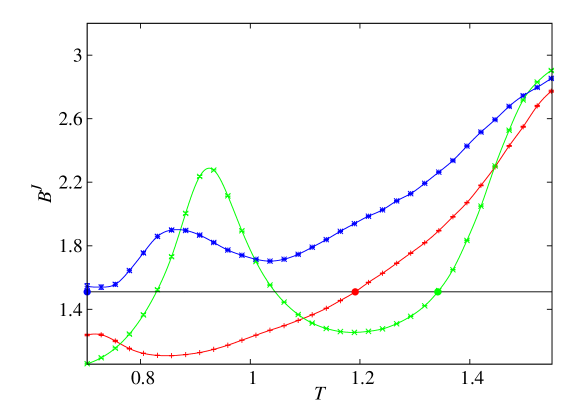
Figure 1: Computation of the pseudo-critical temperature using the Binder ratio defined in eq. 9. Here $y=1.51$, that is a good approximation to $B(T_{\text{c}})$, and we plot $B^{J}(T)$ for three samples with $L=32$. The red curve has exactly one solution (in our range) for $B^{J}(T)=y$, which defines its $T_{y=1.51}^{J}$: this is the normal behaviour of this observable. The green sample has three solutions, so we pick the largest one (green dot). The blue sample has $B^{J}(T)>y$: in this case we take the lowest simulated temperature $T\approx 0.7$ as an upper bound for the pseudo-critical temperature (this ignorance will not affect our estimate for the median). Error bars are included in the plot and are very small.

For each value of $L$ we can search for the temperature $T_{c,y}^{L}$ such that

$$O(T_{c,y}^{L},L)=y\;.$$ (14)

Then, provided we are not very far from the scaling region (so that $y$ is not too different from $y_{\text{c}}$), we expect that

$$T_{c,y}^{L}\simeq T_{\text{c}}+A_{y}L^{-1/\nu}(1+B_{y}L^{-\omega})\;,$$ (15)

where we have included the first corrections to scaling.

We can use this same approach to define a single-sample critical temperature $T_{\text{c}}^{J}$. Let us choose a fixed value of $y$ close enough to the value $y_{\text{c}}$ defined from the sample average at the critical point. For each sample we use cubic splines to determine $T_{y}^{L,J}$ such that

$$O^{J}(T_{y}^{L,J},L)=y\;.$$ (16)

For some samples the $O^{J}(T,L)$ turn out not to be monotonic: there can be several solutions to this equation. In those cases we simply pick the largest solution. This process is illustrated in Figure 1.

The motivation for this choice is simple. The physical meaning of a pseudo-critical temperature is a characteristic temperature that separates the paramagnetic phase from the low-temperature one. Indeed, any temperature $T_{y}^{J}$, solving the equation $O^{J}(T_{y},L)=y$, is a temperature where non-paramagnetic behaviour has already arisen. Therefore, only the largest $T_{y}^{J}$ makes sense as a divider among both phases. In fact, the non-monotonic behaviour of $O^{J}(T,L)$ may be due to other reasons (in particular, temperature chaos), unrelated to the paramagnetic/spin-glass phase transition. In any case, our definition will be justified a posteriori, on the view of the simplicity of the emerging physical picture.

The values of $T_{y}^{J}$ have a very wide probability distribution. For a few disorder samples the solution of eq. (16) falls out of our simulated range of temperatures and we only obtain an upper or (less frequently) a lower bound (see the blue curve in Figure 1). In this situation the arithmetic average of the $T_{y}^{J}$ is not well defined: we consider instead the median temperature, that we denote by $\tilde{T}_{y}^{J}$. Since, by definition, the median does not change as long as the proportion of samples without a solution is less than 50%, this is a robust estimator in these circumstances (we are well below this limit for all the cases considered, the typical proportion being about $\sim 1\%$). From fig. 1 it is also clear that the statistical uncertainty over the determination of $T_{y}^{J}$ in a given sample is very small as compared to the size of sample to sample fluctuations.

In analogy with the sample averaged case (15), we make the ansatz

$$\tilde{T}_{y}^{J}(L)\simeq T_{\text{c}}+A_{y}L^{-1/\nu}\;,$$ (17)

where we have ignored sub-leading corrections. A fit to this equation would, in principle, yield the values of $T_{\text{c}}$ and $\nu$. However, for a fixed value $y$, we do not have enough degrees of freedom to determine simultaneously $\nu$ and $T_{\text{c}}$.

Following the approach of janus:10b , we get around this problem by considering $n$ values of $y$ at the same time: this allows us to fit at the same time all the resulting $\tilde{T}_{y}^{J}(L)$, with fit parameters $\{T_{\text{c}},\nu,A_{y_{1}},\ldots,A_{y_{n}}\}$: in other words we force the $\tilde{T}_{y}^{J}$ obtained for different $y$ values to extrapolate to the same $T_{\text{c}}$ with the same exponent. This procedure may seem dangerous, since we are extracting several transition temperatures from each of the $O^{J}(T,L)$, that are correlated variables. However, the effect of these correlations can be controlled by considering the complete covariance matrix of the data.

The set of points $\{\tilde{T}_{y_{i}}^{J}(L_{a})\}$ are labelled by their $L$ and their $y$: we have data for ${\cal L}=5$ different values of $L$, with $L_{1}=8$, $L_{2}=12$, $L_{3}=16$, $L_{4}=24$, $L_{5}=32$ ($4000$ samples in all cases but for $L=32$, where we have $1000$). We also select $n$ values of $y_{i}$ in the critical region ($y_{1}$, $\ldots$, $y_{n}$). The appropriate chi-square estimator is

$$\chi^{2}=\sum_{i,j=1}^{n}\sum_{a,b=1}^{\cal L}\bigl{[}\tilde{T}_{y_{i}}^{J}(L_{a})-T_{\text{c}}-A_{y_{i}}L_{a}^{-1/\nu}\bigr{]}\sigma^{-1}_{(ia)(jb)}\bigl{[}\tilde{T}_{y_{j}}^{J}(L_{b})-T_{\text{c}}-A_{y_{j}}L_{b}^{-1/\nu}\bigr{]}\;,$$ (18)

where $\sigma_{(ia)(jb)}$ is the covariance matrix of the set of $T_{y}^{J}$, which we compute by a bootstrap approach boostrap (each point of the set is identified by $L$ and $y$): it is a block-diagonal matrix, since the data for different $L$ values are uncorrelated.

Thus far we have considered just a single observable $O$, for different values of $y$. Since the fitting function (17) is the same for the different $O$ we have selected, with common $T_{\text{c}}$ and $\nu$, and only amplitudes differ, we can include in the same fit data for the four dimensionless quantities (8–11), considering several values of $y$ for each. In order to simplify the notation, from here on we shall denote our set of points in the fit as $\{\tilde{T}_{\alpha}^{J}(L)\}$, taking $\alpha$ as labelling both the observable $O$ and the height $y$ (so that it will range from $1$ to $4\,n$).

We can use the usual disorder averaged spin-glass susceptibility $\chi_{\mathrm{SG}}$ to arrive at yet another determination of the single-sample critical temperature, with the definition

$$\chi_{\text{SG}}^{J}(T^{J}_{\chi})=\chi_{\mathrm{SG}}(T_{\mathrm{c}})\;y\;,$$ (19)

with $y$ close to one, and we expect $\tilde{T}^{J}_{\chi}$ to follow the same scaling behaviour of (17): we include the values of $\tilde{T}^{J}_{\chi}$ in the global fit to the individual pseudo critical temperatures. In this case the pathologies that affect the analysis of other single sample observables are far less frequent.

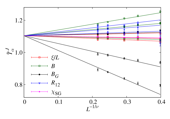
Figure 2: Global fit for the median single-sample critical temperature $\tilde{T}_{\alpha}^{J}$ computed with different observables. The parameters in the fit are the common extrapolation point $T_{\text{c}}$, the common exponent $\nu$ and an individual amplitude for each set of data points. We include in the fit the data for $L\geq 12$.

We show the results of this combined fitting procedure in Figure 2, where we have included data for the four dimensionless ratios $\xi/L$, $B$, $B_{G}$ and $R_{12}$, using three values of $y$ for each ratio (we plot the three fits for the same observable with the same colour). We have also used the data for $T_{\chi}^{J}$, with $y=1$ (we select the value of $T_{\text{c}}$ reported in hasenbusch:08b ). We have discarded the $L=8$ data, which showed strong corrections to the leading scaling of (17). The best fit gives

$$T_{\text{c}} =1.104(6)\;, \nu =2.26(13)\;,$$ (20)

with $\chi^{2}=32.6$ for $37$ degrees of freedom (giving a $P$ value of $68\%$). This results nicely agree with the determination of hasenbusch:08b ,

$$T_{\text{c}} =1.109(10), \nu =2.45(15).$$ (21)

Ref. hasenbusch:08b includes corrections to scaling, as in (15), with $\omega=1.0(1)$. Ref. K1 gives a comprehensive list of estimates for $T_{c}$ and $\nu$. In order to take these scaling corrections into account and to include the $L=8$ data in the fit, we can therefore rewrite (17) as

$$\tilde{T}_{\alpha}^{J}(L)\simeq T_{\text{c}}+A_{\alpha}L^{-1/\nu}(1+B_{\alpha}L^{-\omega}),$$ (22)

where again we use the same $\omega$ parameter for all the observables and all values of $y$. Unfortunately, our numerical data are not precise enough to allow a reliable determination of $\omega$, $\nu$ and $T_{\text{c}}$ at the same time (the resulting error in $\omega$ would be greater than $100\%$). We have been able to check consistency of our approach by taking the values of $\nu$ and $\omega$ from hasenbusch:08b and fitting only for $T_{\text{c}}$ and for the amplitudes, including now the data for $L=8$. The resulting best fit gives $T_{\text{c}}=1.105(8)$, with $\chi^{2}=41.9$ for $38$ degrees of freedom ($P$ value: $35\%$): this is a satisfactory check of consistency.

The results we have discussed make us confident of the fact that our determination of the single-sample critical temperatures yields reasonable results. We can now take the analysis one step further and consider the width of the distribution of $T_{\text{c}}^{J}$. We consider the two temperatures $T^{+}_{\alpha}$ and $T^{-}_{\alpha}$ such that

$$P(T_{\alpha}^{J}>T_{\alpha}^{+}) =0.16\;, P(T_{\alpha}^{J}<T_{\alpha}^{-}) =0.16\;.$$ (23)

The value $0.16$ is such that the temperature interval $[T_{\alpha}^{-},T_{\alpha}^{+}]$ defines the same probability as an interval of two standard deviations around the mean for a Gaussian probability distribution. We define the width $\Delta T_{\alpha}^{J}$ as

$$\Delta T_{\alpha}^{J}=\frac{T^{+}_{\alpha}-T^{-}_{\alpha}}{2}\;.$$ (24)

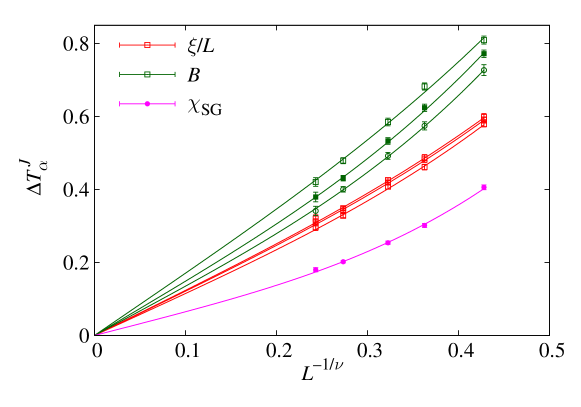
Figure 3: Global fit to $\Delta T_{\alpha}^{J}$, computed using $\xi^{J}/L$, $B^{J}$ and $\chi_{\text{SG}}^{J}$.

The simplest ansatz for the scaling behaviour of $\Delta T_{\alpha}^{J}$ is

$$\Delta T_{\alpha}^{J}\simeq A_{\alpha}L^{-1/\nu}(1+B_{\alpha}L^{-\omega})\;.$$ (25)

In principle we could repeat the global fitting procedure that we have applied to the medians $\tilde{T}_{\alpha}^{J}$. Unfortunately, not all the observables that we considered in Figure 2 can be used to analyse $\Delta T_{\alpha}^{J}$, since the distribution of some of them is too wide, so that the critical temperature of too many samples falls out of our simulated range of $T$, and the width defined in eq. 25 is undefined. Because of that we analyse $\Delta T_{\alpha}^{J}$ by only using the $T_{y}^{J}$ derived from $\xi^{J}/L$, $B^{J}$ and $\chi_{\text{SG}}^{J}$. The corrections to scaling are now stronger than for the median $\tilde{T}_{y}^{J}$, so that we cannot obtain a good fit to leading order even if we discard the data for $L=8$. Using once again as an input the critical exponents from hasenbusch:08b and fitting for the amplitudes we obtain a very good fit with $\chi^{2}=19.1$ for $21$ degrees of freedom ($P$ value: $58\%$). The results of the best fit are plotted in Figure 3. According to the ansatz of eq. 2, the width of $T_{y}^{J}$ must be equal to the width of ${T_{\mathrm{c}}^{J}(L)}$ (since $C_{y}$ is $J$ independent): the width of $T_{y}^{J}$ should accordingly be $y$ independent. Figure 3 shows that this is indeed the case for $\Delta T_{\xi/L}^{J}$, but less so for $\Delta T_{B}^{J}$: as mentioned before the disorder independence of the scaling function in eq. 2 is only approximate Domany .

III The Sherrington-Kirkpatrick mean field theory

The Hamiltonian of the Sherrington-Kirkpatrick mean field model is

$$H_{\text{SK}}\equiv-\frac{1}{\sqrt{N}}\sum_{i,j}S_{i}\,J_{i,j}\,S_{j}\;,$$ (26)

where the sum runs over all couples of spins of the system, the Ising $S_{i}$ spin variables can take the two values $\pm 1$ and the couplings are quenched binary variables that can take the value $\pm 1$ with probability one half.

III.1 The pseudo-critical temperatures

Our analysis of the mean field SK model is very similar to the one we have discussed in the case of the Edwards-Anderson model. Here we have seven values of the system size $N$ (of the form $N=2^{p}$, with $p$ ranging from $6$ to $12$: in all cases we have $1024$ disorder samples but for $N=4096$ where we have $256$ and for $N=128$ where we have $8192$), that makes the fitting procedure stable. It is also of use the fact that in this case the value of the (infinite volume) critical temperature, $T_{c}=1$ is known exactly.

We consider three definitions of $T_{\mathrm{c}}$:

• the one based on the single sample Binder cumulant of eq. 9, $B^{J}(T^{J}_{B})=B(T_{\mathrm{c}})$;

• one based on the low order cumulant $D=E(\langle q^{2}\rangle)/E(\langle|q|\rangle)^{2}$ and the single sample quantity $D^{J}={\langle q^{2}\rangle_{J}}/{\langle|q|\rangle^{2}_{J}}$, i.e. $D^{J}(T^{J}_{D})=D(T_{\mathrm{c}})$;

• one based on the spin-glass susceptibility $\chi_{SG}^{J}(T^{J}_{\chi})=\chi_{\mathrm{SG}}(T_{\mathrm{c}})$.

For a given value of $N$, we use for the left hand sides $B(T_{\mathrm{c}})$, $D(T_{\mathrm{c}})$ and $\chi_{\mathrm{SG}}(T_{\mathrm{c}})$ the values measured for this same size, at $T_{\mathrm{c}}=1$. We solve eq. (16) by using a simple linear interpolation.

Like for the EA model, in some cases eq. (16) can have more than one solution. We again choose the largest solution, which in the case of SK turns out to be always the one closer to the infinite volume value $T_{\mathrm{c}}$. In a few cases, for small values of $N$, the equation has only solutions outside the range of temperatures that was used in the parallel tempering Monte Carlo simulation ($0.4\leq T\leq 1.30$). We fix this problem again by basing our statistical analysis on the median of the distribution and on the definition of the width given by eq. 24. It turns out that these pathological cases are less numerous for the SK model than for the EA model, and that the width given by eq. 24 is always defined.

In terms of the number of sites $N$ of the SK fully connected lattice the ansatz of eq. 17 becomes

$$\tilde{T}_{y}^{J}(L)\simeq T_{\text{c}}+A_{y}N^{-1/(\nu d_{\text{up}})}=T_{\text{c}}+A_{y}N^{-1/3}\;.$$ (27)

We show in fig. 4 the data for the median of the distribution of $T^{J}_{\chi}$ as a function of $1/N^{1/3}$, together with the results of two best fits. We first notice that the data are well compatible with the fact that in the $N\to\infty$ limit $T_{c}=1$. The first fit is a linear fit to the form $T^{J}_{\chi}=1+a/N^{1/3}$ (with $N\geq 256$ and $\chi^{2}=4.44$ with $4$ degrees of freedom). This is a good fit for the large systems, but it fails below $N=256$. We also show a (very good) best fit including the next to leading corrections, with an exponent $2/3$ (including all $N$ values, $\chi^{2}=2.07$ with $5$ degrees of freedom). The analysis of the data for $T^{J}_{B}$ and $T^{J}_{D}$ leads to the same conclusions: here however the leading term ($\propto 1/N^{1/3}$) has a small coefficient and the effect of the next to leading term is stronger. In conclusion our data are in excellent agreement with an asymptotic $1+{\cal O}(1/N^{1/3})$ behaviour for the median of the distribution.

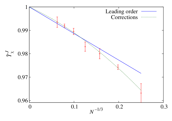
Figure 4: The median of the distribution of $T^{J}_{\chi}$ as function of $1/N^{1/3}$, together with the results of two best fits: a leading order fit, and a fit including a higher order correction (see text).

We show in fig. 5 the width of the distribution of $T^{J}_{\chi}$ as a function of $1/N^{1/3}$, together with the results of two fits, namely $\Delta T_{\chi}^{J}=c_{1}/N^{1/3}$, and $\Delta T_{\chi}^{J}=c_{1}N^{-1/3}+c_{2}N^{-2/3}$ respectively. The data are well compatible with $\Delta T=0$ in the limit $N\to\infty$, as expected. The leading order fit, including $N\geq 256$, has a $\chi^{2}=5.36$ with $4$ degrees of freedom. The two-parameter fit gives an excellent representation of the data (with a $\chi^{2}=2.475$ with $5$ degrees of freedom) including now the $N=64$ and $N=128$ points. Very similar results are obtained for $\Delta T_{B}^{J}$ and $\Delta T_{C}^{J}$.

In conclusion our finite size, numerical analysis of the SK model strongly support an asymptotic ${\cal O}(N^{-1/3})$ scaling behaviour for the width of the distribution of the pseudo-critical temperatures.

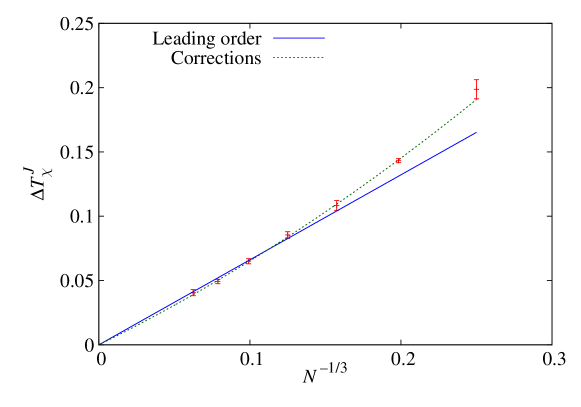
Figure 5: The width of the distribution of $T^{J}_{\chi}$ as function of $N^{-1/3}$, together with the results of two fits: a leading order fit, and a fit including a higher order correction (see text).

III.2 Scaling with the system size and the stability of TAP states

Our results are in contradiction with the claim made in Castellana that the width of the finite-size fluctuations due to quenched disorder of the critical temperature of the SK spin glass scales like $N^{-2/3}$. We show here that we can give support to our numerical finding by means of a very simple scaling argument.

The SG susceptibility can be computed from the TAP free energy Thouless:77 as

$$\chi_{\mathrm{SG}}=\frac{1}{N}\mathrm{Tr}\mathcal{M}^{-2}\;,$$ (28)

where ${\cal M}$ is the Hessian of the TAP free energy at the relevant minimum. If we seat deep in the paramagnetic phase, the only relevant minimum of the TAP free energy is $m_{i}=0$ for all $i=1,2,\ldots,N$. Note that in the pseudo-critical region, where $(\beta-\beta_{\mathrm{c}})N^{1/3}\sim 1$, is not at all obvious that the such TAP solution is the relevant one (for instance a sub-extensive set of sites of size $N^{\alpha}$, with $\alpha<1$, could have non-vanishing $m_{i}$, or maybe one could have for all sites $|m_{i}|\sim N^{-\alpha^{\prime}}$, with $\alpha^{\prime}>0$): the following discussion is relevant only in the paramagnetic phase and for system sizes so large that $(\beta_{\mathrm{c}}-\beta)\gg N^{-1/3}$.

It was shown some time ago Mike that, at $\beta=\beta_{\mathrm{c}}$, the smallest eigenvalue of the Hessian at the fully-paramagnetic TAP solution is of order $N^{-2/3}$. In Ref. Castellana it has been argued that

$$\lambda_{\mathrm{min},J}=(1-\beta)^{2}+\frac{\beta}{N^{2/3}}\Phi^{(N)}_{J}\,,$$ (29)

where $\Phi_{J}^{(N)}$ is a random variable that, in the limit of large $N$, converges in distribution to a Tracy-Widom random-variable TW . In particular, note that at the critical temperature $\beta_{\mathrm{c}}=1$ the $N^{-2/3}$ scaling is recovered.

Now, only for the purpose of discussing the crudest features of the scaling laws, let us assume that $\chi_{\mathrm{SG}}$ is dominated by the contribution of the smallest eigenvalue:

$$\chi_{\mathrm{SG}}^{J} \sim \frac{1}{N\lambda_{\mathrm{min},J}^{2}}\,,$$ (30)

$$= \frac{1}{N\left((1-\beta)^{2}+\frac{\beta}{N^{2/3}}\Phi^{(N)}_{J}\right)^{2}}\,,$$ (31)

$$= N^{1/3}\frac{1}{\left(\left[N^{1/3}(1-\beta)\right]^{2}+\beta\Phi^{(N)}_{J}\right)^{2}}\,.$$ (32)

The analysis of Ref. Castellana is based entirely on eq. (31).

Now, note that eq. (32) implies that interesting behaviour appears only when $(1-\beta)\leq 1/N^{1/3}$: this makes sensible to replace $\beta\Phi^{(N)}_{J}$ with $\Phi^{(N)}_{J}$. At this point, an implication emerges for the scaling with $N$ of the average susceptibility. We have that

$$\chi_{\mathrm{SG}}(T,N)=N^{1/3}G\bigl{(}N^{1/3}(1-\beta)\bigr{)}\;,$$ (33)

where the scaling function $G$ has the form

$$G(x)=\int_{-\infty}^{+\infty}\,\mathrm{d}\Phi\,p_{\mathrm{TW}}(\Phi)\,\frac{1}{(x^{2}+\Phi)^{2}}\,.$$ (34)

In the above expression $p_{\mathrm{TW}}(\Phi)$ is the Tracy-Widom probability density function.

Eq. (34) is not acceptable for two main reasons:

• the function $G(x)$ in eq.(34) is ill-defined, as the integrand has a non-integrable singularity at $\Phi=-x^{2}$;

• if one devises some regularisation procedure, dimensional analysis would indicate that $G(x)\sim x^{-4}$ in the limit of large $x$. However, in order to recover the correct critical divergence $\chi_{\mathrm{SG}}^{N=\infty}\sim 1/(1-\beta)$, one obviously needs $G(x)\sim 1/x$.

The solution of these two caveats is of course in the fact that the initial assumption, $\chi_{\mathrm{SG}}^{J}\sim 1/(N\lambda_{\mathrm{min},J}^{2})$, is incorrect. The contribution of $\sim N$ eigenvalues is crucial in order to recover the correct scaling behaviour $G(x)\sim 1/x$. Thus, the only lesson that we may take from this oversimplified analysis is that the $J$-dependent SG susceptibility will probably scale as

$$\chi_{\mathrm{SG}}^{J}=N^{1/3}\mathcal{F}\left(\left[N^{1/3}(1-\beta)\right]+\Psi_{J}^{(N)}\right)\,.$$ (35)

This is exactly the scaling ansatz we made at the beginning, where $\Psi_{J}^{(N)}$ is some random-variable that (in distribution) remains of order $1$ in the large-$N$ limit. This result is consistent with our numerical findings.

Merely rewriting eq. (31) as eq. (32) suffices to make it obvious that the asymptotic statement in Ref. Castellana is incorrect: the width of the distribution of the pseudo-critical temperatures scales with $N^{-1/3}$. Indeed, if as done in Ref. Castellana , one simply derives in eq. (31) with respect to $\beta$ in order to get the maximum of the susceptibility, one finds that $1-\beta_{\mathrm{c},J}\sim N^{-2/3}$. But at such value of $\beta_{\mathrm{c},J}$ we have that $(1-\beta)^{2}\sim N^{-4/3}\ll\frac{\beta}{N^{2/3}}\Phi^{(N)}_{J}$, In other words, at the scale of $(1-\beta)\sim 1/N^{2/3}$ eq. (31) predicts an essentially constant behaviour, hence the supposed maximum of the susceptibility (recall that at such value of $\beta$ the fully paramagnetic TAP minimum is probably no longer the relevant one) has no physical meaning.

III.3 The probability distribution of the pseudo-critical inverse temperatures

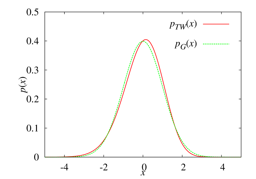
Figure 6: Probability density functions for the Gaussian distribution and for the Tracy-Widom distribution for the Gaussian Orthogonal Ensemble, both with zero average and unitary variance.

We have discussed in some detail about the features of the pseudo-critical, sample dependent temperatures in the mean field SK theory, and we have determined their scaling properties. The next step, that we present here, is in the study of their probability distribution. Unfortunately, there is not any clean analytical prediction for the shape that this distribution function should take in the large-$N$ limit. The only proposal known to us was put forward in ref. Castellana : when properly scaled, the pseudo-critical temperatures should follow a Tracy-Widom (TW) distribution, in our case for the Gaussian Orthogonal Ensemble (GOE). Unfortunately, as we have explained in Sect. III.2, the reasoning leading to that prediction is flawed (although, on the long run, the prediction itself could be correct).

Lacking an analytical guidance, we will simply check whether our numerical data can be described by either a TW distribution, or by the ubiquitous Gaussian distribution. Within our limited statistics and system sizes, the two distributions turn out to be acceptable (the Gaussian hypothesis fits slightly better our data, but a Tracy-Widom hypothesis is certainly consistent as well). Given the preliminary nature of this study, we shall restrict ourselves to the simplest determination of pseudo-critical temperatures, the one coming from the spin-glass susceptibility.

Let us start by noticing that the difference of a Gaussian distribution $F_{G}(\phi)$ and a TW distribution for the GOE $F_{TW}(\phi)$ is indeed very small. We show in figure 6 both a Gaussian and a TW distribution with zero average and variance equal to one: it is clear that they are very similar. Some numerical values can be of help. In the case of zero average and unitary variance a Gaussian has a fourth moment equal to $3$, as opposed to $3.165$ for a TW. The Gaussian is symmetric and has zero skewness, while the TW distribution has a small asymmetry, with a skewness equal to -0.29, The Gaussian has a kurtosis equal to zero, while a TW has a kurtosis equal to $0.165$. We will use these numerical remark at the end of this section for sharpening the outcome of our quantitative analysis.

It is clear that in this situation, where the two target distributions are very similar, one has to keep under very strong control finite size effects, that could completely mask the asymptotic behaviour. It is important to notice that the effects we are looking at characterise not only the tails but the bulk of the distribution.

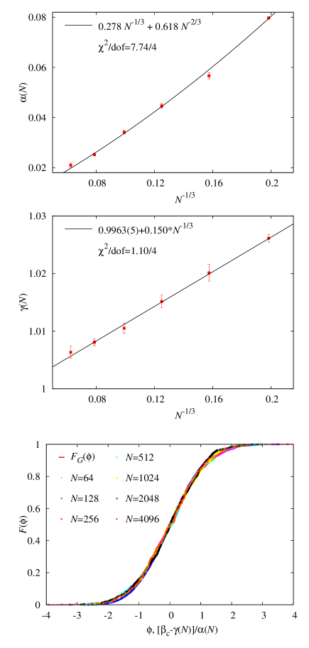
Figure 7: (top): $\alpha(N)$, defined in equation 36, versus $N^{-1/3}$, and our best fit including the first scaling corrections. (middle): $\gamma(N)$, defined in equation 36, versus $N^{-1/3}$, and our best fit. Here the fitting function only includes the leading term, since this form already gives a good value for $\chi^{2}$. (bottom): collapse of the EDF for different $N$ values and of the theoretical distribution function, as described in the text. Here we show the case of a Gaussian distribution.

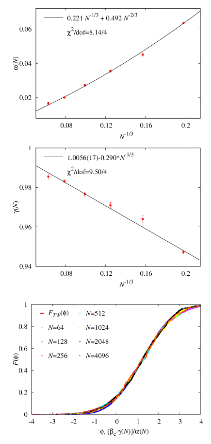
Figure 8: As in figure 7, but for a TW probability distribution.

Let us give the basic elements of our approach. We consider the value of the pseudo-critical inverse temperatures computed from the spin glass susceptibility for different $N$ values. We try to verify if a relation of the form

$$\beta_{c}^{(N)}=\gamma_{N}+\alpha_{N}\,\phi\;,$$ (36)

(where $\phi$ is a random variable with null expectation values and unit variance, Gaussian or TW like) can account for our numerical data and, if yes, to determine the scaling behaviour of $\gamma_{N}$ and of $\alpha_{N}$. We now define the variable $\tilde{\beta_{\mathrm{c}}}\equiv(\beta_{c}-\gamma)/\alpha$. Let us assume that for a system of size $N$ we have $K_{N}$ samples, and therefore $K_{N}$ pseudo-critical temperatures $\tilde{\beta_{\mathrm{c}}}(N,s),s=1,2,\ldots,K_{N}$. The empirical distribution function (EDF) is then

$$H_{N}(\tilde{\beta_{\mathrm{c}}})\equiv\frac{1}{K_{N}}\sum_{s=1}^{K_{N}}\theta(\tilde{\beta_{\mathrm{c}}}-\tilde{\beta_{\mathrm{c}}}(N,s))\,,$$ (37)

where $\theta$ is the Heaviside step function. Note that the parameters $\alpha(N)$ and $\gamma(N)$ in Eq. 36 are unknown a priori. They will be determined through a fitting procedure (see Eq. 38 below). In particular, they typically take different numerical values if we adopt the TW hypothesis, or the Gaussian hypothesis.

We define the distance among the EDF and the theoretical distribution as

$$D\equiv\frac{1}{K_{N}}\sum_{s=1}^{K_{N}}\left[F(\tilde{\beta}_{\mathrm{c}}(N,s))-H_{N}(\tilde{\beta}_{\mathrm{c}}(N,s))\right]^{2}\,.$$ (38)

In order to get an error estimate we repeat the procedure for $1000$ bootstrap samples for each value of $N$. In fig. 7 we consider the theoretical hypothesis of a Gaussian distribution. We show in the top part of the figure $\alpha(N)$ versus $N^{-1/3}$, and our best fit including the first scaling corrections. In the middle frame we show $\gamma(N)$ versus $N^{-1/3}$, and our best fit. Here the fitting function only includes the leading term, since this form already gives a good value for $\chi^{2}$. In the bottom frame we show the collapse of the EDF for different $N$ values and of the theoretical distribution function, as described in the text. In fig. 8 we show the same data for the hypothesis of a TW distribution.

In short, even if the Gaussian hypothesis is slightly favoured over the TW one, this analysis does not allow us to decide clearly in one sense or in the other one. The values of $D$ are always comparable among the two cases. The estimates of $\gamma(N)$ are indeed more consistent for the Gaussian case, but the difference of the quality of the two fits does not allow us to say a clear, final word.

In order to try to sharpen our analysis we have used the Cramer-von Mises criterion Anderson ; Darling ; Darling-par . We will not give here technical details (see, however, endnote noteCvM ), but will only discuss the most important features and the results. When we normalise the distribution to zero average we and unitary width we introduce a correlations about the values to be tested: also because of that we find a better fit to our needs the two sample formulation of the criterion, with a non-parametric approach, where we have to start by fitting the test statistics (since we cannot use tabulated values, because we are determining $\alpha_{N}$ and $\gamma_{N}$ in Eq. 36 from our finite-size statistics). Again, as in our previous analysis, tests do not allow us to select a Gaussian or a TW distribution: they are both characterised by very similar levels of significance.

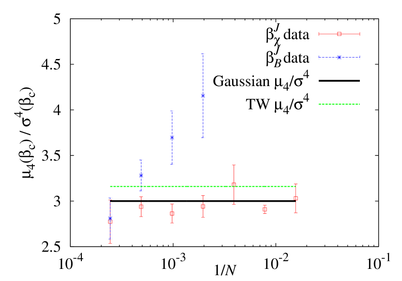
Figure 9: Measured fourth moment of the probability distribution, both for data from $\chi_{SG}$ and for data from the pseudo Binder parameter, versus $1/N$. Thick straight line is for a Gaussian distribution (where the value is three), while the thinner straight line is for a TW distribution.

A very simple analysis is maybe the most revealing. As we have discussed at the start of this section the fourth moment of a normalised Gaussian is equal to three, while the fourth moment of a TW distribution is equal to $3.165$. We plot in fig. 9 the measured fourth moment of the probability distribution, both for data from $\chi_{SG}$ and for data from the pseudo Binder parameter, versus $1/N$. The thick straight line is for a Gaussian distribution (where the value is three), while the thinner straight line is for a TW distribution. Again, these data do not allow for a precise statement, but they seem to favour the possibility of a Gaussian behaviour (the data for $\chi_{SG}$ give maybe the clearer indication).

Our conclusions is that, given the quality of our data and the sizes of our thermalised configurations, that do not go beyond $N=4096$, a Gaussian distribution is favoured, but we cannot give a clear, unambiguous answer.

IV Conclusions

We have presented a simple method to study the probability distribution of the pseudo-critical temperature for spin glasses. We have applied this method to the $3d$ EA Ising spin glass and to the fully connected SK models. Our results are in excellent agreement with a median of the distribution that behaves asymptotically like $T_{\mathrm{c}}+{\cal O}(L^{-1/\nu})$ (or $1+{\cal O}(N^{-1/3})$ for the SK model), and a width of the distribution that behaves like ${\cal O}(L^{-1/\nu})$ (or $1+{\cal O}(N^{-1/3})$ for the SK model). The value of $\nu$ we find for the EA model is compatible with state of the art results. Furthermore, even if our number of samples is modest as compared with Ref. hasenbusch:08b , our determination of $\nu$ and $T_{\mathrm{c}}$ is competitive. An analysis of the probability distribution of the pseudo-critical inverse temperatures for the SK mean field model does not lead to firm conclusions, but hints to a Gaussian behaviour.

- (1) J. A. Mydosh, Spin Glasses: an Experimental Introduction (Taylor and Francis, London 1993)
- (2) K. H. Fisher and J. A. Hertz, Spin Glasses (Cambridge University Press, Cambridge 1993).
- (3) Y. G. Joh et al., Phys. Rev. Lett. 82, 438 (1999).
- (4) R. Álvarez Baños, A. Cruz, L. A. Fernandez, J. M. Gil-Narvion, A. Gordillo-Guerrero, M. Guidetti, A. Maiorano, F. Mantovani, E. Marinari, V. Martin-Mayor, J. Monforte-Garcia, A. Muñoz Sudupe, D. Navarro, G. Parisi, S. Perez-Gaviro, J. Ruiz-Lorenzo, S. F. Schifano, B. Seoane, A. Tarancon, R. Tripiccione and D. Yllanes (Janus Collaboration), J. Stat. Mech. 2010, P06026.
- (5) R. Álvarez Baños, A. Cruz, L. A. Fernandez, J. M. Gil-Narvion, A. Gordillo-Guerrero, M. Guidetti, A. Maiorano, F. Mantovani, E. Marinari, V. Martin-Mayor, J. Monforte-Garcia, A. Muñoz Sudupe, D. Navarro, G. Parisi, S. Perez-Gaviro, J. Ruiz-Lorenzo, S. F. Schifano, B. Seoane, A. Tarancon, R. Tripiccione and D. Yllanes (Janus Collaboration), Phys. Rev. Lett. 105, 177202 (2010).
- (6) D. J. Amit and V. Martin-Mayor, Field Theory, the Renormalization Group and Critical Phenomena (World Scientific, Singapore 2005).
- (7) See e.g. L. Berthier et al., Science 310, 1797 (2005), and references therein.
- (8) A. B. Harris, J. Phys. C 7, 1671 (1974).
- (9) A. Aharony and A. B. Harris, Phys Rev Lett 77, 3700 (1996).
- (10) F. Pázmándi, R. T. Scalettar and G. T. Zimányi, Phys. Rev. Lett. 79, 5130 (1997).
- (11) S. Wiseman and E. Domany, Phys. Rev. Lett. 81, 22 (1998); Phys Rev E 58, 2938 (1998).
- (12) A. Aharony, A. B. Harris and S. Wiseman, Phys. Rev. Lett. 81, 252 (1998).
- (13) K. Bernardet, F. Pázmándi and G. G. Batrouni, Phys. Rev. Lett. 84, 4477 (2000).
- (14) S. Wiseman and E. Domany, Phys Rev E 52, 3469 (1995).
- (15) J. T. Chayes, L. Chayes, D. S. Fisher and T. Spencer, Phys. Rev. Lett. 57, 2999 (1986).
- (16) T. Sarlat, A. Billoire, G. Biroli and J.-P. Bouchaud, J. Stat. Mech. P08014 (2009).
- (17) M. Castellana and E. Zarinelli, Phys. Rev. B 84, 144417 (2011).
- (18) M. Castellana, A. Decelle and E. Zarinelli, preprint arXiv:1107.1795.
- (19) A. Billoire and B. Coluzzi (2006), unpublished.
- (20) G. Parisi, F. Ritort and F. Slanina, J. Phys. A: Math. Gen. 26, 247 (1993).
- (21) We are assuming that in the low temperature phase, i.e. for example that we are working with an infinitesimal magnetic field.
- (22) T. Aspelmeier, A. Billoire, E. Marinari and M. A. Moore, J. Phys. A 41, 324008 (2008).
- (23) See for example B. Efron and R. J. Tibshirani, An Introduction to the Boostrap (Chapman & Hall/CRC,London 1994).
- (24) M. Hasenbusch, A. Pelissetto and E. Vicari, Phys. Rev. B 78, 214205 (2008).
- (25) H. G. Katzgraber, M. Körner and A. P. Young, Phys. Rev. B 73, 224432 (2006).
- (26) D. J. Thouless, P. W. Anderson and R. G. Palmer, Philos. Mag. 35, 593 (1977).
- (27) A. J. Bray and M. A. Moore, J. Phys. C: Solid State Phys. 12, L441 (1979).
- (28) C. A. Tracy and H. Widom, Comm. Math. Phys. 177, 727 (1996); M. Dieng, Distribution functions for edge eigenvalues in orthogonal and symplectic ensembles: Painlevé representation PhD thesis, UC Davis (2005), arXiv:math/0506586; P. Deift and D.Gioev, Comm. Pure Appl. Math. 60, 867 (2007), arXiv:math-ph/0507023.
- (29) T. W. Anderson, Ann. Math. Statist. 33, 1148 (1962).
- (30) D. A. Darling, Ann. Math. Statist. 28, 823 (1957).
- (31) D. A. Darling, Ann. Math. Statist. 26, 1 (1955).
- (32) Given two independent samples of and values respectively of a random variable , whose empirical distribution functions are and , and being the empirical distribution function of the sample obtained by combining the two original samples together, the two-samples Cramér-von Mises statistics is the distance .