Quantization of the interior Schwarzschild black hole

Abstract

We study a Hamiltonian quantum formalism of a spherically symmetric space-time which can be identified with the interior of a Schwarzschild black hole. The phase space of this model is spanned by two dynamical variables and their conjugate momenta. It is shown that the classical Lagrangian of the model gives rise the interior metric of a Schwarzschild black hole. We also show that the the mass of such a system is a Dirac observable and then by quantization of the model by Wheeler-DeWitt approach and constructing suitable wave packets we get the mass spectrum of the black hole.
PACS numbers: 04.70.-s, 04.70.Dy, 04.60.Ds
Keywords: Quantum black hole, interior Schwarzschild black hole, Dirac observables

1 Introduction

Black hole physics has played a central role in conceptual discussion of general relativity in classical and quantum levels. For example regarding event horizons, space-time singularities and also studying the aspects of quantum field theory in curved space-time. In classical point of view, the horizon of a black hole which is a one way membrane, and the space-time singularities are some interesting features of the black hole solutions in general relativity [1]. In spirit of the Ehrenfest principle, any classical adiabatic invariant corresponds to a quantum entity with discrete spectrum, Bekenstein conjectured that the horizon area of a non extremal quantum black hole should have a discrete eigenvalue spectrum [2]. Also, the black hole thermodynamics is based on applying quantum field theory to the curved space-time of a black hole [3]. According to this formalism, the Hawking radiation of a black hole is due to random processes in the quantum fields near the horizon. The mechanism of this thermal radiation can be explained in terms of pair creation in the gravitational potential well of the black hole [4]. The conclusions of the above works are that the temperature of a black hole is proportional to the surface gravity and that the area of its event horizon plays the role of its entropy. In this scenario, the black hole is akin to a thermodynamical system obeying the usual thermodynamic laws, often called the laws of black hole mechanics, first formulated by Hawking [3]. In more recent times, this issue has been at the center of concerted efforts to describe and make clear various aspects of the problem that still remain unclear, for a review see [5]. With the birth of string theory [6], as a candidate for quantum gravity and loop quantum gravity [7], a new window was opened to the problem of black hole radiation. This was because the nature of black hole radiation is such that quantum gravity effects cannot be neglected [8]. According to all of the above remarkable works, it is believed that a black hole is a quantum mechanical system and thus like any other quantum system its physical states can be described by a wavefunction. Indeed, due to its fundamental conceptual role in quantum general relativity, we may use it as a starting point for testing different constructions of quantum gravity [9, 10].

On the other hand, studying the interior of the Schwarzschild black hole is interesting for various reasons [11]. Many authors expressed the idea that the interior of a black hole can be considered as an anisotropic cosmological model [12]. In this direction, the author of [13] used it as a cosmological model to describe time dependent cosmological constant. One of the most important and interesting cosmological usage of the interior solution is considering black hole as a spawn of mother universe so that our universe was born from it as a daughter universe [14]. Many cosmological models in which our universe emerges from the interior of a black hole have been proposed in [15]. From a mathematical point of view, the space-time metric of the interior of a black hole can be constructed from its exterior metric. Indeed, one of the interesting features of general relativity is to generate cosmological solutions from known static solutions of the Einstein field equations. The methods from which one finds such solutions are investigated in [16]. Generally, these methods are based on a diffeomorphism between the known static solutions and the corresponding cosmological model. For example, the coordinate transformation $t\leftrightarrow r$ converts the Schwarzschild metric to a dynamical model which can be identified with its inside space-time. Indeed, at the horizon of a Schwarzschild black hole the light cone tips over and for $r<r_{s}$, $\partial/\partial r$ become time-like while $\partial/\partial t$ become space-like. This means that inside the black hole the metric has time-dependent coefficients. Thus, one can use this correspondence to make a quantum theory of black holes based on a quantized cosmological model.

In this letter we deal with the Hamiltonian formalism of a time-dependent spherically symmetric space-time. We show that the classical solutions of such a dynamical system can be identified with the interior space-time of a Schwarzschild black hole. In this model the metric functions play the role of independent dynamical variables which with their conjugate momenta construct the corresponding phase space. We then consider a Hamiltonian quantum theory by replacing the classical phase space variables by their Hermitian operators. We study the various aspects of the resulting quantum model and corresponding Wheeler-DeWitt (WD) equation and present closed form expressions for the wavefunction of the black hole. We shall see that the quantum solutions also represent a quantization rule for the mass of the black hole. In what follows, we work in units where $c=\hbar=1$.

2 The model

We start with the Einstein-Hilbert action

$${\cal S}=\frac{1}{16\pi G}\int d^{4}x\sqrt{-g}{\cal R}+S_{YGH},$$ (1)

where ${\cal R}$ is the Ricci scalar, $g$ is the determinant of the metric tensor and $S_{YGH}$ is the York-Gibbons- Hawking boundary term . We assume that the geometry of space-time is described by a spherically symmetric metric with time-dependent line element as

$$ds^{2}=-\frac{N^{2}(t)}{\nu(t)}dt^{2}+\nu(t)dr^{2}+h^{2}(t)(d\vartheta^{2}+\sin^{2}\vartheta d\varphi^{2}),$$ (2)

where $N(t)$ is the lapse function, while $\nu(t)$ and $h(t)$ are functions of $t$ only, which play the role of our dynamical variables to construct the phase space. It is clear that the above metric with $t=\mbox{const.}$ and $r=\mbox{const.}$ describes the surface of a $2$-sphere with radius $h(t)$ and area $A=4\pi h^{2}(t)$. By substituting (2) into (1) and integrating over spatial dimensions, we are led to an effective Lagrangian in the minisuperspace $(\nu,h)$ as

$${\cal L}=-\frac{V_{0}}{8\pi G}\left[\frac{1}{N}\left(h\dot{h}\dot{\nu}+\dot{h}^{2}\nu\right)-N\right],$$ (3)

in which $V_{0}$ is the volume of the space part of the action where is treated to be a finite constant. A point $(\nu,h)$ in this minisuperspace represents a $4$-geometry. Although, in this step we can vary the above Lagrangian to get the equation of motion for $h$ and $\nu$, but the Hamiltonian constraint resulting from this Lagrangian does not have the desired form for construction of WD equation describing the relevant quantum model. Thus, to transform Lagrangian (3) to a more manageable form, consider the following change of variables

$$x-y=h,\hskip 14.22636ptx+y=h\nu.$$ (4)

In terms of these new variables, Lagrangian (3) takes the form

$${\cal L}=-\frac{V_{0}}{8\pi G}\left[\frac{1}{N}\left(\dot{x}^{2}-\dot{y}^{2}\right)-N\right].$$ (5)

Now, if we use the following coordinate transformation which is introduced in [12]

$$\begin{array}[]{cc}(x-y)^{\frac{1}{2}}=\frac{1}{2}(u-v),\\ \\ (x+y)^{\frac{1}{2}}=\frac{1}{2}(u+v),\end{array}$$ (9)

and the lapse rescaling

$$N=(x^{2}-y^{2})^{\frac{1}{2}}\widetilde{N},$$ (10)

then the corresponding Lagrangian becomes

$${\cal L}=-{M^{2}_{Pl}V_{0}}\widetilde{N}^{-1}(\dot{u}^{2}-\dot{v}^{2})+{M_{Pl}^{2}V_{0}}\widetilde{N}(u^{2}-v^{2}),$$ (11)

which describes an isotropic oscillator-ghost-oscillator system.

To construct the Hamiltonian of the model, note that the momenta conjugate to $u$ and $v$ are

$$\begin{array}[]{cc}\Pi_{u}=-\frac{2V_{0}M^{2}_{Pl}}{\widetilde{N}}\dot{u},\\ \\ \Pi_{v}=\frac{2V_{0}M^{2}_{Pl}}{\widetilde{N}}\dot{v}.\end{array}$$ (15)

Also, the primary constraint is given by

$$\Pi_{\widetilde{N}}=\frac{\partial{\cal L}}{\partial\dot{\widetilde{N}}}=0.$$ (16)

In terms of the conjugate momenta the Hamiltonian is given by

$$H=\dot{u}\Pi_{u}+\dot{v}\Pi_{v}-{\cal L},$$ (17)

leading to

$$H=-\frac{\widetilde{N}}{4M^{2}_{Pl}V_{0}}(\Pi_{u}^{2}-\Pi_{v}^{2})-V_{0}M^{2}_{Pl}\widetilde{N}(u^{2}-v^{2}).$$ (18)

Because of the existence of constraint (16), the Lagrangian of the system is singular and the total Hamiltonian can be constructed by adding to $H$ the primary constraints multiplied by arbitrary functions of time $\lambda(t)$

$$H_{T}=-\frac{\widetilde{N}}{4M^{2}_{Pl}V_{0}}(\Pi_{u}^{2}-\Pi_{v}^{2})-V_{0}M^{2}_{Pl}\widetilde{N}(u^{2}-v^{2})+\lambda\Pi_{\widetilde{N}}.$$ (19)

The requirement that the primary constraint should hold during the evolution of the system means that

$$\dot{\Pi}_{N}=\left\{\Pi_{N},H_{T}\right\}\approx 0,$$ (20)

which leads to the secondary (Hamiltonian) constraint

$${\cal H}=-\frac{1}{4V_{0}M_{Pl}^{2}}(\Pi_{u}^{2}-\Pi_{v}^{2})-{V_{0}M_{Pl}^{2}}(u^{2}-v^{2})\approx 0.$$ (21)

Before going any further, some remarks are in order about the mass of the system. In the usual classical theory, the unique solution to the vacuum Einstein equation for the spherically symmetric space-time is the Schwarzschild solution in which there exists an integration constant representing the mass of the black hole. In the canonical formalism for the spherically symmetric space-time, by following Fischler-Morgan-Polchinski [17] and Kuchar [18] calculations the mass of a black hole can be regarded as a dynamical variable, which can be expressed as a function of canonical data. The spherically symmetric hypersurface on which the canonical data is given is supposed to be embedded in a Schwarzschild black hole space-time whose metric is given by

$$N=1,\hskip 14.22636pt\nu=\frac{2MG}{t}-1,\hskip 14.22636pth=t.$$ (22)

This identification of the space-time with the canonical data enables us to connect the Schwarzschild mass $M$ with the canonical data on any small piece of a space-like hypersurface. As a result, from combination of the relations (4), (9), (15) and (22) the mass function can be expressed by the canonical variables as

$$M=\frac{\pi}{2V_{0}}\left(\frac{1}{4M^{2}_{Pl}V_{0}}\left(\Pi_{u}+\Pi_{v}\right)^{2}+V_{0}M^{2}_{Pl}(u-v)^{2}\right).$$ (23)

It is easy to show that the Poisson bracket of mass function with the Hamiltonian vanishes strongly

$$\{M,{\cal H}\}=0,$$ (24)

which shows that the mass is a constant of motion.

3 Classical solutions

The setup for constructing the phase space and writing the Lagrangian and Hamiltonian of the model is now complete. The classical dynamics is governed by the variation of Lagrangian (11) with respect to $u$ and $v$, that is

$$\ddot{u}+\widetilde{N}^{2}u=0,\hskip 14.22636pt\ddot{v}+\widetilde{N}^{2}v=0.$$ (25)

Up to this point the model, in view of the concerning issue of time, has been of course under-determined. Before trying to solve these equations we must decide on a choice of time in the theory. The under-determinacy problem at the classical level may be removed by using the gauge freedom via fixing the gauge. A glance at the above equations shows that a suitable gauge is $\widetilde{N}=M_{Pl}$ which results the following equations

$$\ddot{u}+M^{2}_{Pl}u=0,\hskip 14.22636pt\ddot{v}+M^{2}_{Pl}v=0.$$ (26)

Choosing some parameters $\theta_{1}$ and $\theta_{2}$ as the integration constants, the solutions are obtained as

$$u=A\cos(M_{Pl}t+\theta_{1}),\hskip 14.22636ptv=B\cos(M_{Pl}t+\theta_{2}),$$ (27)

where $A$ and $B$ are constants to be determined later. Now, the above solutions should satisfy the constraint of a vanishing Hamiltonian. Thus, substitution (27) into (21) gives a relation between the constants $A$ and $B$

$$A=\pm B,$$ (28)

implying that we can rewrite the solutions (27) as

$$u=A\cos(M_{Pl}t+\theta_{1}),\hskip 14.22636ptv=A\eta\cos(M_{Pl}t+\theta_{2}),$$ (29)

where $\eta$ takes the values $\pm 1$ according to the choices in (28). Since in the quantum version of the model we are interested in constructing wave packets from the WD equation, we would like to obtain a classical trajectory in configuration space $(u,v)$, where the classical time $t$ is eliminated. This is because no such parameter exists in the WD equation. It is easy to see that the classical solutions (29) may be displayed as the following trajectories

$$u^{2}+v^{2}-2\eta\cos(\Delta\theta)uv-A^{2}\sin^{2}(\Delta\theta)=0,$$ (30)

where $\Delta\theta=\theta_{1}-\theta_{2}$. Equation (30) describes ellipses which their major axes make angle $\pi/4$ with the positive/negative $u$ axis according to the choices $\pm 1$ for $\eta$. Also, the eccentricity and the size of each trajectory are determined by $\Delta\theta$ and $A$ respectively.

On the other hand, inserting solution (27) into the mass function, we obtain

$$M=2\pi M^{2}_{Pl}A^{2}\sin(\frac{\Delta\theta}{2}).$$ (31)

To obtain the usual Schwarzschild solution, consider time rescaling $Ndt=d\tau$, where from (10) we have $N=M_{Pl}(u^{2}-v^{2})/4$. Consequently, solutions (27) give

$$\cos(2M_{Pl}t+\theta_{1}+\theta_{2})=\frac{-8(\tau-\tau_{0})}{A^{2}\sin\Delta\theta},$$ (32)

where $\tau_{0}$ is a constant of integration. From equations (4) and (9) one then has

$$\begin{array}[]{cc}h=\begin{cases}-2\coth(\frac{\Delta\theta}{2})\tau,\hskip 14.22636pt\eta=1,\hskip 8.5359pt\Delta\theta<0,\\ 2\tanh(\frac{\Delta\theta}{2})\tau,\hskip 14.22636pt\eta=-1,\hskip 8.5359pt\Delta\theta>0.\\ \end{cases}\end{array}$$ (34)

and

$$\nu=\begin{cases}\cot^{2}(\frac{\Delta\theta}{2})\left(\frac{2GM}{\tau}\cot(\frac{\Delta\theta}{2})-1\right),\hskip 14.22636pt\eta=1,\hskip 14.22636pt\Delta\theta<0,\\ \tan^{2}(\frac{\Delta\theta}{2})\left(\frac{2GM}{\tau}\tan(\frac{\Delta\theta}{2})-1\right),\hskip 14.22636pt\eta=-1,\hskip 14.22636pt\Delta\theta>0,\\ \end{cases}$$ (35)

in which we put

$$\begin{array}[]{cc}\tau_{0}=-\frac{\eta}{8}A^{2}\sin\Delta\theta.\end{array}$$ (37)

Thus, in terms of the metric functions $(h,\nu)$ the classical trajectories (30) take the form

$$\nu=\frac{1}{2}\left(\frac{A^{2}\sin^{2}\Delta\theta}{1-\eta\cos\Delta\theta}\right)\frac{1}{h}-\left(\frac{1+\eta\cos\Delta\theta}{1-\eta\cos\Delta\theta}\right).$$ (38)

Therefore, the above Lagrangian formalism leads us to the following interior Schwarzschild black hole metric if we assume $\Delta\theta=2n\pi-\pi/2$ when $\eta=1$ and $\Delta\theta=2n\pi+\pi/2$ when $\eta=-1$, respectively

$$ds^{2}=-\left(\frac{2MG}{\tau}-1\right)^{-1}d\tau^{2}+\left(\frac{2MG}{\tau}-1\right)dr^{2}+\tau^{2}\left(d\vartheta^{2}+\sin^{2}\vartheta d\varphi^{2}\right).$$ (39)

It is clear from the condition $\nu(\tau)>0$ that this solution is only valid for $\tau<2MG$. The above metric has an apparent singularity at $\tau=2MG$. This singularity is like the coordinate singularity associated with horizon in the Schwarzschild or de Sitter space-time, and as is well known, there are other coordinate system for which this type of singularity is removed [1]. Another singularity associated with the metric (39) is its essential singularity at $\tau=0$. As we know, in general relativity, to investigate the types of singularities one has to study the invariants characteristics of space time and to find where these invariants become infinite so that the classical description of space-time breaks down. In a 4- dimensional Riemannian space-time there are $14$ independent invariants, but to detecting the singularities it is sufficient to study only three of them, the Ricci scalar ${\cal R}$, $R_{\mu\nu}R^{\mu\nu}$ and the so-called Kretschmann scalar $R_{\mu\nu\sigma\delta}R^{\mu\nu\sigma\delta}$. For the metric (39) the Kretschmann scalar reads

$$K=R_{\mu\nu\sigma\delta}R^{\mu\nu\sigma\delta}=\frac{48G^{2}M^{2}}{\tau^{6}}.$$ (40)

Now, it is clear that the space-time describing by the metric (39) has an essential singularity at $\tau=0$, where can not be removed by a coordinate transformation. Note that the Schwarzschild manifold contains an anisotropic expanding universe, the white hole portion of the extended geometry, and also an anisotropic collapsing universe, the black hole interior as well. In this paper we focus attention on the black hole interior portion of the geometry, but all conclusions may be restated in terms of the expanding white hole geometry due to the time reversal symmetry of both Schwarzschild geometries.

4 Dirac Observables

As is well known general relativity is invariant under the group of diffeomorphisms of the space-time manifold ${\cal M}$. The main consequences of such a diffeomorphism invariance are that the Hamiltonian can be expressed as a sum of constraints and any observable must commute with these constraints. An observable is a function on the constraint surface such that is invariant under the gauge transformations generated by all of the first class constraints. By a first class constraint we mean a phase space function with the property that it has weakly vanishing Poisson bracket with all constraints. As an example the momentum and Hamiltonian constraints are always first class, see (16) and (21). The Hamiltonian and momentum constraints in general relativity are generators of the corresponding gauge transformations, and so a function on the phase space is an observable if has weakly vanishing Poisson brackets with the first class constraints. To find gauge invariant observables, we can proceed as follows. In Lagrangian (11), the unconstrained phase space $\Gamma$ is $\mathbb{R}^{4}$ with global canonical coordinates $(x_{i},\Pi_{i})$, $i=1,2$, with Poisson brackets $\{x_{i},\Pi_{j}\}=\delta_{ij}$. Now, let us define on $\Gamma$ the complex-valued functions

$$\begin{array}[]{cc}C_{i}=M_{Pl}\sqrt{V_{0}}x_{i}+i\frac{1}{2M_{Pl}\sqrt{V_{0}}}\Pi_{i},\\ \\ C^{*}_{i}=M_{Pl}\sqrt{V_{0}}x_{i}-i\frac{1}{2M_{Pl}\sqrt{V_{0}}}\Pi_{i},\end{array}$$ (44)

where $x_{i}=\{u,v\}$ and $\Pi_{i}=\{\Pi_{u},\Pi_{v}\}$. The set $S=\{C_{i},C^{*}_{i},1\}$ on $\Gamma$ is closed under the Poisson bracket, $\{C_{i},C^{*}_{j}\}=-i\delta_{ij}$ and every sufficiently regular function on $\Gamma$ can be expressed in terms of the sums and products of the elements of $S$. Hence, the Hamiltonian and mass can be viewed as

$${\cal H}=C^{*}_{v}C_{v}-C^{*}_{u}C_{u},$$ (45)

and

$$M=\frac{\pi}{2V_{0}}\left(C_{u}-C^{*}_{v}\right)\left(C^{*}_{u}-C_{v}\right).$$ (46)

Therefore, the classical Poisson algebra generated by the elements of $S$ is sufficiently large for describing the classical dynamics of the system. In the next section we will use this algebra as the starting point for quantization of the model. The classical dynamics of these variables is

$$\begin{array}[]{cc}C_{u}=AV_{0}^{\frac{1}{2}}M_{Pl}^{2}e^{i(t+\theta_{1})},\\ \\ C_{v}=\eta AV_{0}^{\frac{1}{2}}M_{Pl}^{2}e^{-i(t+\theta_{2})}.\end{array}$$ (50)

To find a set of constraints of motion, consider on $\Gamma$ the functions

$$\begin{array}[]{cc}J_{0}=-\frac{1}{2}(C^{*}_{v}C_{v}+C^{*}_{u}C_{u}),\\ \\ J_{+}=C_{v}C_{u},\\ \\ J_{-}=C^{*}_{v}C^{*}_{u},\end{array}$$ (56)

whose Poisson brackets form a closed algebra by

$$\begin{array}[]{cc}\{J_{+},J_{-}\}=2iJ_{0},\\ \\ \{J_{0},J_{\pm}\}=\mp iJ_{\pm}.\end{array}$$ (60)

The elements of this algebra have strongly vanishing Poison brackets with the Hamiltonian. Since the physical space is two dimensional, there will be at most two independent constraints. On the constraint surface ${\cal H}=0$, the functions $J$’s are not algebraically independent but satisfy the identity

$$J_{0}^{2}-J_{+}J_{-}=0.$$ (61)

Also, we can write the mass function as a combination of $J$’s as

$$M=-\frac{\pi}{2V_{0}}(2J_{0}+J_{+}+J_{-}).$$ (62)

Thus, the quantity $M$ is a gauge invariant observable.

5 Quantization of the model

We now focus attention on the study of the quantization of the model described above. The quantum version of the model described by relations $\{x_{i},\Pi_{j}\}=\delta_{ij}$ can be achieved via the canonical quantization procedure which leads the following commutation relations

$$[u,\Pi_{u}]=i,\hskip 14.22636pt[v,\Pi_{v}]=i.$$ (63)

Then, the set of hermitian quantum operators $\hat{S}=\{C_{i},C_{i}^{\dagger},1\}$ will have the following commutator algebra

$$\begin{array}[]{cc}[C_{i},C_{j}^{\dagger}]=\delta_{ij}1,\hskip 14.22636pt[C_{i},1]=[C^{\dagger}_{i},1]=0.\end{array}$$ (65)

The set $\hat{S}$ and its commutator algebra are the quantum counterpart of the set $S$ and its Poisson bracket algebra. The operator version of the classical Hamiltonian constraint takes the form

$$H=C_{v}^{\dagger}C_{v}-C_{u}^{\dagger}C_{u}.$$ (66)

Let us define vacuum state according to

$$C_{u}|0,0>=0,\hskip 14.22636ptC_{v}|0,0>=0,$$ (67)

so that $C_{i}$ and $C_{i}^{\dagger}$ are annihilation and creation operators respectively. Note that by the Hamiltonian operator (66), zero point energy is canceled out. Consequently, the WD equation can be written as

$$H\Psi(u,v)=\left(-\frac{\partial^{2}}{\partial u^{2}}+\frac{\partial^{2}}{\partial v^{2}}+\omega^{2}(u^{2}-v^{2})\right)\Psi(u,v)=0,$$ (68)

where $\omega=V_{0}/8\pi G$. This equation is a quantum isotropic oscillator-ghost-oscillator system with zero energy. Therefore, its solutions belong to a subspace of the Hilbert space spanned by separable eigenfunctions of a two-dimensional isotropic simple harmonic oscillator Hamiltonian. Separating the eigenfunctions of (68) in the form

$$\Phi_{n_{1},n_{2}}(u,v)=X_{n_{1}}(u)Y_{n_{2}}(v),$$ (69)

yields

$$\begin{array}[]{cc}X_{n_{1}}(u)=\left(\frac{\omega}{\pi}\right)^{1/4}\left[\frac{H_{n_{1}}(\omega^{1/2}u)}{\sqrt{2^{n_{1}}n_{1}!}}\right]e^{-\omega u^{2}/2},\\ \\ Y_{n_{2}}(v)=\left(\frac{\omega}{\pi}\right)^{1/4}\left[\frac{H_{n_{2}}(\omega^{1/2}v)}{\sqrt{2^{n_{1}}n_{2}!}}\right]e^{-\omega v^{2}/2}.\end{array}$$ (73)

subject to the restriction $n_{1}=n_{2}=n$. In (73), $H_{n}(x)$ are Hermite polynomials and the eigenfunctions are normalized according to

$$\int_{-\infty}^{+\infty}e^{-x^{2}}H_{n}(x)H_{m}(x)dx=2^{n}\pi^{1/2}n!\delta_{mn}.$$ (74)

The set $\{\Phi_{n_{1},n_{2}}(u,v)\}$ forms a closed span of the zero sector subspace of the Hilbert space $L_{2}$ of measurable square-integrable functions on $\mathbb{R}^{2}$ with the usual inner product defined as

$$\int\Phi_{n_{1},n_{2}}(u,v)\Phi_{m_{1},m_{2}}(u,v)dudv=\delta_{n_{1},m_{1}}\delta_{n_{2},m_{2}},$$ (75)

that is, the orthonormality and completeness of the basis functions follow from those of the Hermite polynomials. Therefore, in the position representation, we may write the general solution of the WD equation as a superposition of the above eigenfunctions

$$\Psi(u,v)=\left(\frac{\omega}{\pi}\right)^{1/2}\sum_{n=0}^{\infty}\frac{c_{n}}{2^{n}n!}e^{-\frac{\omega}{2}(u^{2}+v^{2})}H_{n}(\sqrt{\omega}u)H_{n}(\sqrt{\omega}v).$$ (76)

where $c_{n}$ are a set of complex constants. In general, one of the most important features in quantum WD approach is the recovery of classical solutions from the corresponding quantum model or, in other words, how can the WD wavefunctions predict a classical model. In this approach, one usually constructs a coherent wave packet with good asymptotic behavior in the minisuperspace, peaking in the vicinity of the classical trajectory. Therefore, for our subsequent analysis, by using the equality

$$\sum_{n=0}^{\infty}\frac{s^{n}}{n!}H_{n}(x)H_{n}(y)=\frac{1}{\sqrt{1-s^{2}}}\exp\left[\frac{2xys-s^{2}(x^{2}+y^{2})}{2(1-s^{2})}\right],$$ (77)

we can evaluate the sum over $n$ in (76) and simple analytical expression for this sum is found if we choose the coefficients $c_{n}$ to be $c_{n}=B2^{n}\tanh\zeta$, where $B$ and $\zeta$ are arbitrary complex constants, which results in

$$\begin{array}[]{cc}\Psi(x,y)={\cal N}\exp[-\frac{1}{4}\cos(2\beta)\cosh(2\alpha)(x^{2}+y^{2}-2\eta\tanh(2\alpha)xy)]\\ \\ \times\exp[-\frac{i}{4}\sinh(2\alpha)\sin(2\beta)(x^{2}+y^{2}-2\eta\coth(2\alpha)xy)].\end{array}$$ (81)

In this expression $\alpha$ and $\beta$ are the real and imaginary parts of $\zeta$ respectively, that is, $\zeta=\alpha+i\beta$, $x=\sqrt{\omega}u$, $y=\sqrt{\omega}v$ and ${\cal N}$ is a numerical factor. In figure 1 we have plotted the square of the wavefunction for typical values of the parameters in which we have taken the following combination of the solutions

$$\Phi(x,y)=\Psi_{\eta,\alpha,\beta}(x,y)-\Psi_{\eta,\alpha+\delta\alpha,\beta+\delta\beta},$$ (82)

for some $\delta\alpha$ and $\delta\beta$ in the vicinity of $\alpha$ and $\beta$. It is seen that a good correlation exists between the quantum pattern shown in this figure and the classical trajectories (30) in configuration space $(u,v)$.

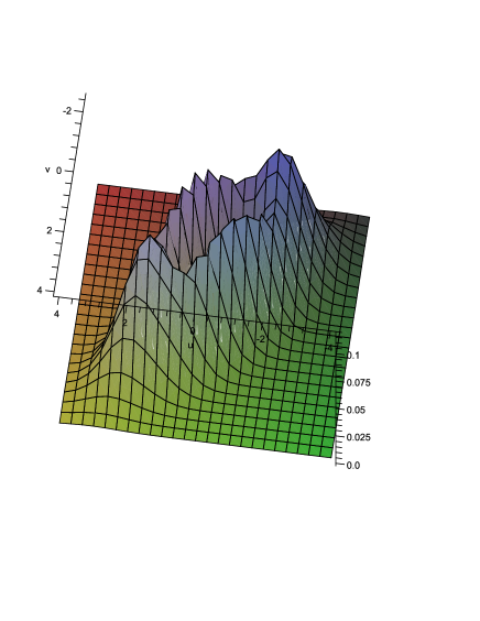
Figure 1: The figure shows $|\Phi(x,y)|^{2}$ the square of the wavefunction. This figure is plotted for numerical values $\alpha=1$, $\delta\alpha=0.3$, $\beta=\pi/4$, $\delta\beta=3\pi/20$, $\eta=1$ and $\omega=1$.

In continuation of this section we focus attention on the Dirac observables of the black hole and try to build an algebra of physical operators, that is, a subalgebra of ${\cal A}$ that would leave $V_{HH,0}$ invariant. To do this, notice that the Poisson bracket algebra of the classical $J$’s can be promoted into a commutator algebra version by setting

$$J_{+}=C_{v}C_{u},\hskip 14.22636ptJ_{-}=C_{v}^{\dagger}C_{u}^{\dagger},\hskip 14.22636ptJ_{0}=-\frac{1}{2}\left(C_{v}^{\dagger}C_{v}+C_{u}^{\dagger}C_{u}+1\right),$$ (83)

so that the corresponding commutators are

$$[J_{+},J_{-}]=2J_{0},\hskip 14.22636pt[J_{0},J_{\pm}]=\mp J_{\pm}.$$ (84)

Equations (84) are recognized as the commutators of the Lie algebra of $SO(2,1)$. Since all these operators commute with Hamiltonian $H$, we choose our physical operator algebra to be the algebra generated by the set $\{J_{\pm},J_{0},1\}$. Note that in analogy to the classical algebraic identity (61) the quantum $J$’s are not independent and satisfy the following algebraic relation

$$J_{0}^{2}-\frac{1}{2}(J_{+}J_{-}+J_{-}J_{+})+\frac{1}{4}=0.$$ (85)

Now, the action of the operators $\{C_{i},C_{i}^{\dagger}\}$ on the states of the physical Hilbert space is

$$\begin{array}[]{cc}C_{u}|n_{1},n_{2}>=\sqrt{n_{1}}|n_{1}-1,n_{2}>,\hskip 14.22636ptC_{u}^{\dagger}|n_{1},n_{2}>=\sqrt{n_{1}+1}|n_{1}+1,n_{2}>,\\ \\ C_{v}|n_{1},n_{2}>=\sqrt{n_{2}}|n_{1},n_{2}-1>,\hskip 14.22636ptC_{v}^{\dagger}|n_{1},n_{2}>=\sqrt{n_{2}+1}|n_{1},n_{2}+1>,\end{array}$$ (89)

so that with the help of (83), one can put the action of $J$’s on the physical states as

$$\begin{array}[]{cc}J_{0}|n_{1},n_{2}>=-\frac{1}{2}(n_{1}+n_{2}+1)|n_{1},n_{2}>,\\ \\ J_{+}|n_{1},n_{2}>=\sqrt{n_{1}n_{2}}|n_{1}-1,n_{2}-1>,\\ \\ J_{-}|n_{1},n_{2}>=\sqrt{(n_{1}+1)(n_{2}+1)}|n_{1}+1,n_{2}+1>,\end{array}$$ (95)

with constraint $n_{1}=n_{2}$. Consequently the expectation value of mass operator for the interior solution will be

$$<M>_{n}=\left(\frac{\pi}{V_{0}}\right)\left(n+\frac{1}{2}\right),$$ (96)

which means that black hole is quantized in discrete states with energies $E_{n}$, that is (in ordinary units)

$$E_{n}=\frac{\pi c\hbar}{V_{0}}\left(n+\frac{1}{2}\right).$$ (97)

It is well known that the parameter $M$ in the outside of a black hole is measured at spatial infinity where the Newtonian approximation is valid and so it is a measure of mass of the black hole. In this sense, we know that the energy spectrum of a quantized black hole from an outside observer point of view is (see [2] and [20])

$$E_{n}=M_{Pl}c^{2}\sqrt{n},$$ (98)

which gives the following relation for the difference between two nearby states

$$\Delta E=\frac{M_{Pl}c^{2}}{\sqrt{n+1}+\sqrt{n}}.$$ (99)

Now, it is obvious that $\Delta E$ tends to zero as $n\rightarrow\infty$ which is in agreement with the correspondence principle and the black hole can be described classically in this regime. On the other hand, the physical meaning of black hole mass parameter may be different inside the event horizon. As equation (97) shows, the energy eigenvalues consist of equally spaced spectrum which resemble the energy spectrum of the harmonic oscillator. This is not surprising, since a decomposition of the quantum fields inside the black hole into normal modes is essentially a decomposition into harmonic oscillators that are decoupled. Also, from (97) we see even the lowest energy level, i.e. the level $n=0$, has some nonzero energy, the so called ground state energy. The existence of such a energy level is a purely quantum mechanical effect and may be interpreted in terms of the uncertainty principle. Indeed, it is this zero-point energy that is responsible for the fact that the system under consideration (interior of the black hole in our case) does not ”freeze” at extremely low energies. Another feature of the result (97) is its agreement with the correspondence principle in the sense that $\frac{E_{n+1}}{E_{n}}\rightarrow 1$ as $n\rightarrow\infty$. As the quantum number $n$ increases the system tends to its classical regime which in this case is a superposition of the eigenstates of the type (76). Such a so-called coherent state consists of unblurred wave packets which minimize the uncertainty relation.

6 Conclusions

It is interesting to investigate how the interior of a black holes would be quantized. Discrete spectra arise in quantum mechanics in the presence of a periodicity in the classical system, which in turn leads to the existence of an adiabatic invariant or action variable. Boher-Somerfeld quantization implies that this adiabatic invariant has an equally spaced spectrum in the semi-classical limit. Using this approach one can determine the mass and the area spectrum of the black holes in view of an outside observer [19]. In this paper we have evaluated analytically the mass spectrum of the interior Schwarzschild black hole by implementing WD equation. The corresponding phase space of the interior of a Schwarzschild black hole is spanned by two dynamical variables and their conjugate momenta. We have shown that the classical Lagrangian of the model gives rise the interior of Schwarzschild solution. Then, we studied quantization of the model through WD equation and by imposing suitable conditions on the solutions of WD equation we have obtained the mass spectrum of the interior of the black hole. Our result shows that the mass spectrum, not only is discrete, but also is equally spaced.

References

-
[1]
S.W. Hawking and G.F.R. Ellis, The large scale
structure of space time, (Cambridge University Press, Combridge,
England, 1973)
R. M. Wald, General relativity, (Chicago University Press, Chicago, 1984) -
[2]
J.D. Bekenstein, Phys. Rev. D 7 (1973) 2333
J.D. Bekenstein, Phys. Rev. D 9 (1974) 3292
J.D. Bekenstein, Nuovo Cimento 11 (1974) 467 -
[3]
J.M. Bardeen, B. Carter and S.W. Hawking, Commun. Math. Phys. 31 (1973) 161
S.W. Hawking, Commun. Math. Phys. 43 (1975) 199
G.W. Gibbons and S.W. Hawking, Phys. Rev. D 15 (1977) 2752 - [4] N.D. Birrell and P.C.W. Davies, Quantum Fields in Curved Space (Cambridge University Press, UK, 1982)
- [5] T. Padmanabhan, Phys. Rep. 406 (2005) 49
-
[6]
N. Seiberg and E. Witten, J. High Energy Phys. 9 (1999) 032
G.T. Horowitz, New J. Phys. 7 (2005) 201 - [7] A. Ashtekar, New J. Phys. 7 (2005) 198
-
[8]
S. Mukherji and S.S. Pal, J. High Energy Phys. 205 (2002) 026 (arXiv: hepth/
0205164)
A. Ashtekar and K. Krasnov, in Black holes, Gravitational Radiation and the Universe, eds. B. Iyer and B. Bhawal (Kluwer Dodrecht, 1999) 149 (arXiv: gr-qc/9804039) -
[9]
J. Louko and J. Mäkelä, Phys. Rev. D 54 (1996) 4982
J. Mäkelä, Schroedinger Equation of the Schwarzschild Black Hole (arXiv: gr-qc/9602008)
J. Mäkelä and P. Repo, Phys.Rev. D 57 (1998) 4899 (arXiv: gr-qc/9708029)
B. Vakili, Int. J. Theor. Phys. (2011), DOI 10.1007/s10773-011-0887-7 (arXiv: arXiv:1102.1682 [gr-qc]) -
[10]
C. Kiefer, J. Marto and P.V. Moniz, Ann. Phys. (Berlin) 18 (2009) 722
(arXiv: 0812.2848 [gr-qc])
K. Nakamura, S. Konno, Y. Oshiro and A. Tomimatsu, Prog. Theor. Phys. 90 (1993) 861 (arXiv: gr-qc/9308029)
M. Kenmoku, H. Kubotani, E. Takasugi and Y. Yamazaki, Phys. Rev. D 59 (1999) 124004 (arXiv: gr-qc/9810042)
B.-B. Wang, Gen. Rel. Grav. 41 (2009) 1181
J.C. Lopez-Domingues, O. Obregon and M. Sabido, Phys. Rev. D 74 (2006) 084024 (arXiv: hep-th/0607002)
O. Obregon, M. Sabido and V.I. Tkach, Gen. Rel. Grav. 33 (2001) 913 (arXiv: gr-qc/0003023)
M. Kenmoku, H. Kubotani, E.Takasugi and Y. Yamazaki, Phys. Rev. D 57 (1998) 4925 (arXiv: gr-qc/9711039) -
[11]
R. Doran, F.S.N. Lobo and P. Crawford, Found. Phys. 38 (2008) 160 (arXiv: gr-qc/0609042)
T.M. Nieuwenhuizen, Exact solution for the interior of a black hole (arXiv: 0805.4169 [gr-qc]) - [12] R.W. Brehme, Am. J. Phys. 45 (1977) 423
- [13] H. Culetu, Int. J. Mod. Phys. A 24 (2009) 1593
- [14] D.A. Easson and R.H. Brandenberger, J. High Energy Phys. 0106 (2001) 024 (arXiv: hep-th/0103019)
-
[15]
V.P. Frolov, M.A. Markov and V.F. Mukhanov, Phys. Lett. B 216 (1989) 272
D. Morgan, Phys. Rev. D 45 (1992) R1005
V. Mukhanov and R. Brandenberger, Phys. Rev. Lett. 68 (1992) 1969 - [16] H. Quevedo and M.P. Ryan, in Mathematical and Quantum Aspects of Relativity and Cosmology, edited by S. Cotsakis and G.W. Gibbons, (Springer Verlag, Berlin, 2000) 191 (arXiv: gr-qc/0305001)
- [17] W. Fischler, D. Morgan, and J. Polchinski, Phys. Rev. D 42 (1990) 4042
- [18] K.V. Kuchar, Phys. Rev. D 50 (1994) 3961
-
[19]
S. Hod, Phys. Rev. Lett. 81 (1998) 4293
O. Dreyer, Phys. Rev. Lett. 90 (2003) 081301 - [20] X.-G. He and B.-Q. Ma, Quantization of Black Holes (arXiv: 1003.2510 [hep-th])