Abstract

We consider incompressible flows between two transversely vibrating solid walls and construct an asymptotic expansion of solutions of the Navier-Stokes equations in the limit when both the amplitude of vibrations and the thickness of the Stokes layer are small and have the same order of magnitude. Our asymptotic expansion is valid up to the flow boundary. In particular, we derive equations and boundary conditions, for the averaged flow. In the leading order, the averaged flow is described by the stationary Navier-Stokes equations with an additional term which contains the leading-order Stokes drift velocity. In a slightly different context (for a flow induced by an oscillating conservative body force), the same equations had been derived earlier by Riley [3]. The general theory is applied to two particular examples of steady streaming induced by transverse vibrations of the walls in the form of standing and travelling plane waves. In particular, in the case of waves travelling in the same direction, the induced flow is plane-parallel and the Lagrangian velocity profile can be computed analytically. This example may be viewed as an extension of the theory of peristaltic pumping to the case of high Reynolds numbers.

1 Introduction

In this paper we study oscillating flows of a viscous incompressible fluid between two solid walls produced by the transverse vibrations of the walls. It is well-known that high-frequency oscillations of the boundary of a domain occupied by a viscous fluid generate not only an oscillating flow but also a (relatively) weak steady flow, which is usually called the steady streaming (see, e.g., the review papers [1] and [2, 3]). Recently such flows attracted considerable attention in the context of application of steady streaming to micro-mixing [4, 5, 6] and to drag reduction in channel flows [7].

The basic parameters of the problem are the inverse Strouhal number $\epsilon$ and the streaming Reynolds number $R_{s}$, defined as

$$\epsilon=\frac{V_{0}^{*}}{\omega d},\quad R_{s}=\frac{V_{0}^{*2}}{\omega\nu^{*}}$$ (1)

where $V_{0}^{*}$ is the amplitude of the velocity of the oscillating walls, $d$ is the mean distance between the walls, $\omega$ is the angular frequency of the vibrations and $\nu^{*}$ is the kinematic viscosity of the fluid. Parameter $\epsilon$ measures the ratio of the amplitude of the displacement of the vibrating wall to the mean distance between the walls and is assumed to be small: $\epsilon\ll 1$. Note that the relation between the standard Reynolds number $R$ based on $V_{0}^{*}$ and $d$ and the streaming Reynolds number $R_{s}$ is given by $R=V_{0}^{*}d/\nu^{*}=R_{s}/\epsilon$, so that $R_{s}\sim 1$ corresponds to $R\gg 1$ when ${\epsilon}$ is small. The present paper deals with the flow regimes with $R_{s}\sim 1$. This implies that the amplitude of the wall displacement is of the same order of magnitude as the thickness of the Stokes layer.

Steady streaming at $R_{s}\sim 1$ (and even for large $R_{s}$) induced by translational oscillations of a rigid body in a viscous fluid had been studied by many authors (see [8, 9, 10, 11, 12, 13, 14]). In the case of a body in an infinite fluid, the problem can be reduced to an equivalent problem about a fixed body placed in an oscillating flow, which considerably simplifies the analysis. A related problem of steady streaming and mass transport produced by water waves had been treated in [17, 18]) where flow regimes with large $R_{s}$ were considered. Previous studies of flows produced by transverse oscillations of solid walls had been mostly focused on the problem of peristaltic pumping in channels and pipes under the assumption of low Reynolds numbers ($R\ll 1$) and small amplitude-to-wavelength ratio (see, e.g., [15, 16, 6]). Although there are a few paper where the case of large Reynolds numbers ($R\gg 1$) had been considered [4, 5, 7], these studies still correspond to $R_{s}\ll 1$. As far as we know, the flow regimes with $R_{s}\sim 1$ have not been treated before.

The aim of this paper is to construct an asymptotic expansion of the solution of the Navier-Stokes equation in the limit ${\epsilon}\to 0$ and $R_{s}\sim 1$. The procedure includes the derivation of the equations and boundary conditions for a steady component of the flow (steady streaming) that persists everywhere except thin layers near the vibrating walls (whose thickness is of the same order as the amplitude of vibrations). Since the thickness of the Stokes layer $\delta=\sqrt{\nu^{*}/\omega}$ and the amplitude of the displacements of the walls $a$ are of the same order of magnitude, the boundary conditions on the moving walls cannot be transferred to the fixed mean positions of the walls. This is what makes the problem difficult.

To obtain an asymptotic expansion, we employ the Vishik-Lyusternik method (see, e.g., [19, 20]) rather than the standard method of matched asymptotic expansions. In comparison with the latter, the Vishik-Lyusternik method does not require the procedure of matching the inner and outer expansions and the boundary layer part of the expansion satisfies the condition of decay at infinity (in boundary layer variable) in all orders of the expansion (this is not so in the method of matched asymptotic expansions where the boundary layer part usually does not decay and may even grow at infinity). The Vishik-Lyusternik method had been used to study viscous boundary layers at a fixed impermeable boundary by Chudov [21]. Recently, it has been applied to viscous boundary layers in high Reynolds number flows through a fixed domain with an inlet and an outlet [22], to viscous flows in a half-plane produced by tangential vibrations on its boundary [23] and to the steady streaming between two cylinders [24]. A similar technique had been used in [25] to construct an asymptotic expansion in a problem of vibrational convection.

The outline of the paper is as follows. In Section 2, we formulate the mathematical problem. In Section 3, the asymptotic equations and boundary conditions are derived. Section 4 outlines the construction of the asymptotic solution. In Section 5, we consider examples of the steady streaming induced by vibrations of the walls in the form of standing or travelling waves. Finally, discussion of results and conclusions are presented in Section 6.

2 Formulation of the problem

We consider a three-dimensional viscous incompressible flow between two parallel walls produced by normal, periodic (in time) vibrations of the walls. Let ${\bf x}^{*}=(x^{*},y^{*},z^{*})$ be the Cartesian coordinates, $t^{*}$ the time, ${\bf v}^{*}=(u^{*},v^{*},w^{*})$ the velocity of the fluid, $p^{*}$ the pressure, $\rho$ the fluid density, $\nu^{*}$ the kinematic viscosity and $d$ the mean distance between the walls. We introduce the non-dimensional quantities

$$\tau=\omega t^{*},\quad{\bf x}=\frac{{\bf x}^{*}}{d},\quad{\bf v}=\frac{{\bf v}^{*}}{\omega\,a},\quad p=\frac{p^{*}}{\rho\,a\,d\,\omega^{2}},$$

where $\omega$ and $a$ are the angular frequency and the amplitude of the vibrations. In these variables, the Navier-Stokes equations take the form

$${\bf v}_{\tau}+{\epsilon}\,({\bf v}\cdot\nabla){\bf v}=-\nabla p+{\epsilon}^{2}\nu\,\nabla{\bf v},\quad\nabla\cdot{\bf v}=0.$$ (2.1)

where

$${\epsilon}=\frac{a}{d},\quad\nu=\frac{\nu^{*}}{\omega a^{2}}.$$

Parameter ${\epsilon}$ is the ratio of the amplitude of vibrations to the mean distance between the walls, $\nu=R_{s}^{-1}$ where $R_{s}$ is the Reynolds number based on the amplitudes of the velocity and the normal displacement of the vibrating boundary (the streaming Reynolds number). The walls are described by the equations

$$z={\epsilon}\,f(x,y,\tau)\quad{\rm and}\quad z=1+{\epsilon}\,g(x,y,\tau),$$ (2.2)

where $f(x,y,\tau)$ and $g(x,y,\tau)$ are given functions that are $2\pi$-periodic in $\tau$ and have zero mean value, i.e.

$$\bar{f}(x,y)\equiv\frac{1}{2\pi}\int\limits_{0}^{2\pi}f(x,y,\tau)\,d\tau=0,\quad\bar{g}(x,y)\equiv\frac{1}{2\pi}\int\limits_{0}^{2\pi}g(x,y,\tau)\,d\tau=0.$$ (2.3)

We also assume that $f(x,y,\tau)$ and $g(x,y,\tau)$ are periodic both in $x$ and in $y$ with periods $L_{x}$ and $L_{y}$, respectively. Boundary conditions for the velocity at the walls are the standard no-slip conditions:

$${\bf v}\!\bigm{|}_{z={\epsilon}f}=f_{\tau}(x,y,\tau)\,{\bf e}_{z},\quad{\bf v}\!\bigm{|}_{z=1+{\epsilon}g}=g_{\tau}(x,y,\tau)\,{\bf e}_{z}.$$ (2.4)

The incompressibility of the fluid implies that functions $f$ and $g$ must satisfy an additional condition which, in the periodic case, is given by

$$\int\limits_{0}^{L_{x}}\int\limits_{0}^{L_{y}}f(x,y,\tau)\,dx\,dy=\int\limits_{0}^{L_{x}}\int\limits_{0}^{L_{y}}g(x,y,\tau)\,dx\,dy.$$ (2.5)

The non-dimensional equations and boundary conditions depend only on two parameters ${\epsilon}$ and $\nu$. In what follows we are interested in the asymptotic behaviour of periodic solutions of Eqs. (2.1), (2.4) in the limit when ${\epsilon}\to 0$ and $\nu=O(1)$. In other words, we consider the situation where the amplitude of the vibration is small and of the same order as the thickness of the Stokes layer.

It is convenient to separate vertical and horizontal components of the velocity as follows:

$${\bf v}={\bf u}+w\,{\bf e}_{z},\quad{\bf u}=u\,{\bf e}_{x}+v\,{\bf e}_{y},$$

i.e. ${\bf u}$ is the projection of the velocity onto the horizontal plane (the $xy$ plane). We will also use the notation: ${\bf r}=(x,y)$ and ${\bf x}=(x,y,z)$.

We seek a solution of (2.1), (2.4) in the form

$${\bf u}={\bf u}^{r}({\bf r},z,\tau,{\epsilon})+{\bf u}^{a}({\bf r},\xi,\tau,{\epsilon})+{\bf u}^{b}({\bf r},\eta,\tau,{\epsilon}),$$

$$w=w^{r}({\bf r},z,\tau,{\epsilon})+{\epsilon}\,w^{a}({\bf r},\xi,\tau,{\epsilon})+{\epsilon}\,w^{b}({\bf r},\eta,\tau,{\epsilon}),$$

$$p=p^{r}({\bf r},z,\tau,{\epsilon})+p^{a}({\bf r},\xi,\tau,{\epsilon})+p^{b}({\bf r},\eta,\tau,{\epsilon}).$$ (2.6)

Here $\xi=z/\epsilon$ and $\eta=(1-z)/\epsilon$ are the boundary layer variables; all functions are assumed to be periodic in $\tau$, $x$ and $y$ with periods $2\pi$, $L_{1}$ and $L_{2}$, respectively. Functions ${\bf u}^{r}$, $w^{r}$, $p^{r}$ represent a regular expansion of the solution in power series in ${\epsilon}$ (an outer solution), and $\{{\bf u}^{a},w^{a},p^{a}\}$ and $\{{\bf u}^{b},w^{b},p^{b}\}$ correspond to boundary layer corrections (inner solutions) to this regular expansion. We assume that the boundary layer parts of the expansion rapidly decay outside thin boundary layers, namely:

$${\bf u}^{a},w^{a},p^{a}=o(\xi^{-s})\quad{\rm as}\quad\xi\to\infty\quad{\rm and}\quad\quad{\bf u}^{b},w^{b},p^{b}=o(\eta^{-s})\quad{\rm as}\quad\eta\to\infty$$ (2.7)

for every $s>0$. In other words, we require that at a distance of order unity from the wall, the boundary layer corrections are smaller than any power of ${\epsilon}$. This assumption will be verified a posteriori. We begin with the regular part of the expansion.

3 Asymptotic expansion

3.1 Regular part of the expansion

Let

$${\bf v}^{r}={\bf v}^{r}_{0}+{\epsilon}\,{\bf v}^{r}_{1}+{\epsilon}^{2}{\bf v}^{r}_{2}+\dots,\quad p^{r}=p^{r}_{0}+{\epsilon}\,p^{r}_{1}+{\epsilon}^{2}p^{r}_{2}+\dots,$$ (3.1)

where ${\bf v}^{r}={\bf u}^{r}+w^{r}\,{\bf e}_{z}$ and ${\bf v}^{r}={\bf u}^{r}_{k}+w^{r}_{k}\,{\bf e}_{z}$ ($k=0,1,2,\dots$). The successive approximations ${\bf v}^{r}_{k}$, $p^{r}_{k}$ ($k=0,1,2,\dots$) satisfy the equations:

$${\partial}_{\tau}{\bf v}^{r}_{k}=-\nabla p^{r}_{k}+{\bf F}^{r}_{k}({\bf x},\tau),\quad\nabla\cdot{\bf v}^{r}_{0}=0,$$ (3.2)

where ${\bf F}^{r}_{0}({\bf x},\tau)\equiv 0$, ${\bf F}^{r}_{1}({\bf x},\tau)=-({\bf v}^{r}_{0}\cdot\nabla){\bf v}^{r}_{0}$ and

$${\bf F}^{r}_{k}({\bf x},\tau)=-\sum_{j=0}^{k-1}({\bf v}^{r}_{j}\cdot\nabla){\bf v}^{r}_{k-j-1}+\nu\nabla^{2}{\bf v}^{r}_{k-2}\quad(k=2,3\dots).$$

In what follows, we will use the following notation: for any $2\pi$-periodic function $f(\tau)$,

$$f(\tau)=\bar{f}+\tilde{f}(\tau),\quad\bar{f}=\frac{1}{2\pi}\int\limits_{0}^{2\pi}f(\tau)d\tau$$ (3.3)

where $\bar{f}$ is the mean value of $f(\tau)$ and, by definition, $\tilde{f}(\tau)=f(\tau)-\bar{f}$ is the oscillating part of $f(\tau)$ that has zero mean value.

3.1.1 Leading-order equations

Consider Eqs. (3.2) for $k=0$. We seek a solution ${\bf v}^{r}_{0}$ which is periodic in $\tau$. It can be written as

$${\bf v}^{r}_{0}=\bar{{\bf v}}^{r}_{0}+\tilde{{\bf v}}_{0},\quad\tilde{{\bf v}}^{r}_{0}=\nabla\phi_{0}$$ (3.4)

where $\phi_{0}$ has zero mean value and is the solution of the boundary value problem

$$\nabla^{2}\phi_{0}=0,\quad\phi_{0}(x+L_{x},y,z)=\phi_{0}(x,y,z),\quad\phi_{0}(x,y+L_{y},z)=\phi_{0}(x,y,z),$$

$$\phi_{0z}\!\bigm{|}_{z=0}=f_{\tau}(x,y,\tau),\quad\phi_{0z}\!\bigm{|}_{z=1}=g_{\tau}(x,y,\tau).$$ (3.5)

Boundary conditions for $\phi_{0z}$ at $z=0$ and $z=1$ will be justified later. On averaging Eqs. (3.2) for $k=1$, we obtain

$$(\bar{{\bf v}}^{r}_{0}\cdot\nabla)\bar{{\bf v}}^{r}_{0}+\overline{(\tilde{{\bf v}}^{r}_{0}\cdot\nabla)\tilde{{\bf v}}^{r}_{0}}=-\nabla\bar{p}^{r}_{1},\quad\nabla\cdot\bar{{\bf v}}^{r}_{0}=0.$$ (3.6)

Since, according to (3.4), $\tilde{{\bf v}}^{r}_{0}$ is irrotational, we have: $\overline{(\tilde{{\bf v}}^{r}_{0}\cdot\nabla)\tilde{{\bf v}}^{r}_{0}}=\overline{(\nabla\phi_{0}\cdot\nabla)\nabla\phi_{0}}=\nabla\bigl{(}\overline{|\nabla\phi_{0}|^{2}}/2\bigr{)}$. Therefore, we can rewrite (3.6) as

$$(\bar{{\bf v}}^{r}_{0}\cdot\nabla)\bar{{\bf v}}^{r}_{0}=-\nabla\Pi_{0},\quad\nabla\cdot\bar{{\bf v}}^{r}_{0}=0,$$ (3.7)

where $\Pi_{0}=\bar{p}^{r}_{1}+\overline{|\nabla\phi_{0}|^{2}/2}$. Equations (3.7) represent the time-independent Euler equations that describe steady flows of an inviscid incompressible fluid. It will be shown later that boundary conditions for $\bar{{\bf v}}^{r}_{0}$ are

$$\bar{{\bf v}}^{r}_{0}\!\bigm{|}_{z=0}={\bf 0},\quad\bar{{\bf v}}^{r}_{0}\!\bigm{|}_{z=1}={\bf 0}.$$ (3.8)

Thus, $\bar{{\bf v}}^{r}_{0}({\bf x})$ is a steady solution of the Euler equations (3.7), which is periodic in $x$ and $y$ and subject to zero boundary condition at $z=0$ and $z=1$. We choose zero solution:

$$\bar{{\bf v}}^{r}_{0}\equiv{\bf 0}$$ (3.9)

(evidently, it satisfies the Euler equations as well as the boundary conditions). This choice implies that there is no steady streaming in the leading order of the expansion.

3.1.2 First-order equations

Separating the oscillatory part of Eqs. (3.2) for $k=1$, we find that

$${\partial}_{\tau}\tilde{{\bf v}}^{r}_{1}=-\nabla\tilde{p}^{r}_{1}-\widetilde{({\bf v}^{r}_{0}\cdot\nabla){\bf v}^{r}_{0}},\quad\nabla\cdot\tilde{{\bf v}}^{r}_{1}=0,$$ (3.10)

Using (3.9) and the fact that $\tilde{{\bf v}}^{r}_{0}$ is irrotational, (3.10) can be written in the form

$${\partial}_{\tau}\tilde{{\bf v}}^{r}_{1}=-\nabla Q_{1},\quad\nabla\cdot\tilde{{\bf v}}^{r}_{1}=0,$$ (3.11)

where $Q_{1}=\tilde{p}^{r}_{1}+\widetilde{(\nabla\phi_{0})^{2}}/2$. It follows from (3.11) that

$${\bf v}^{r}_{1}=\bar{{\bf v}}^{r}_{1}+\tilde{{\bf v}}_{1},\quad\tilde{{\bf v}}^{r}_{1}=\nabla\phi_{1}$$ (3.12)

where $\phi_{1}$ has zero mean value and is the solution of the problem

$$\nabla^{2}\phi_{1}=0,\quad\phi_{1}(x+L_{x},y,z)=\phi_{1}(x,y,z),\quad\phi_{1}(x,y+L_{y},z)=\phi_{1}(x,y,z),$$

$$\phi_{1z}\!\bigm{|}_{z=0}=a_{1}(x,y,\tau),\quad\phi_{1z}\!\bigm{|}_{z=1}=b_{1}(x,y,\tau),$$ (3.13)

where functions $a_{1}(x,y,\tau)$ and $b_{1}(x,y,\tau)$ will be defined later.

On averaging equation for ${\bf v}^{r}_{3}$ and using (3.4) and (3.9), we find that

$$(\bar{{\bf v}}^{r}_{1}\cdot\nabla)\bar{{\bf v}}^{r}_{1}=-\nabla\Pi^{*}_{3}+\nu\nabla^{2}\bar{{\bf v}}^{r}_{1}-\overline{\tilde{\boldsymbol{\omega}}^{r}_{2}\times\nabla\phi_{0}},\quad\nabla\cdot\bar{{\bf v}}^{r}_{1}=0.$$ (3.14)

where $\Pi^{*}_{3}=\bar{p}^{r}_{3}+\overline{(\nabla\phi_{1})^{2}}/2+\overline{\tilde{{\bf v}}^{r}_{2}\cdot\nabla\phi_{0}}$ and $\tilde{\boldsymbol{\omega}}^{r}_{2}=\nabla\times\tilde{{\bf v}}^{r}_{2}$. It is clear from Eq. (3.14) that in order to obtain a closed equation for $\bar{{\bf v}}^{r}_{1}$, we need to find $\tilde{{\bf v}}^{r}_{2}$.

3.1.3 Second-order equations

Consider Eqs. (3.2) for $k=2$. Averaging yields

$$0=-\nabla\bar{p}^{r}_{2}-\overline{({\bf v}^{r}_{0}\cdot\nabla){\bf v}^{r}_{1}}-\overline{({\bf v}^{r}_{0}\cdot\nabla){\bf v}^{r}_{1}},\quad\nabla\cdot\bar{{\bf v}}^{r}_{2}=0.$$

In view of (3.4), (3.9) and (3.12), the first of these reduces to the equation $\nabla\left(\bar{p}^{r}_{2}+\overline{\nabla\phi_{0}\cdot\nabla\phi_{1}}\right)=0$ that can be integrated to obtain

$$\bar{p}^{r}_{2}=-\overline{\nabla\phi_{0}\cdot\nabla\phi_{1}}+{\rm const}.$$ (3.15)

The oscillatory part of (3.2) for $k=2$ gives us the equations for $\tilde{{\bf v}}^{r}_{2}$:

$$\tilde{{\bf v}}^{r}_{2\tau}=-\nabla Q_{2}-(\tilde{{\bf v}}^{r}_{0}\cdot\nabla)\bar{{\bf v}}^{r}_{1}-(\bar{{\bf v}}^{r}_{1}\cdot\nabla)\tilde{{\bf v}}^{r}_{0},\quad\nabla\cdot\tilde{{\bf v}}^{r}_{2}=0,$$ (3.16)

where $Q_{2}=\tilde{p}^{r}_{2}+\widetilde{\nabla\phi_{0}\cdot\nabla\phi_{1}}$, and we have used (3.4), (3.9) and (3.12). Taking curl of the first equation and using (3.4), we obtain

$$\tilde{\boldsymbol{\omega}}^{r}_{2\tau}=\left[\tilde{{\bf v}}_{0}^{r},\bar{\boldsymbol{\omega}}^{r}_{1}\right]$$ (3.17)

where $\bar{\boldsymbol{\omega}}^{r}_{1}=\nabla\times\bar{{\bf v}}^{r}_{1}$ and where $\left[{\bf a},{\bf b}\right]=({\bf b}\cdot\nabla){\bf a}-({\bf a}\cdot\nabla){\bf b}=\nabla\times({\bf a}\times{\bf b})$ for any divergence-free vector fields ${\bf a}({\bf x})$ and ${\bf b}({\bf x})$. Now let $\boldsymbol{\zeta}({\bf x},\tau)$ be such that

$$\boldsymbol{\zeta}_{\tau}=\tilde{{\bf v}}^{r}_{0},\quad\bar{\boldsymbol{\zeta}}={\bf 0}.$$ (3.18)

Then, it follows from (3.17) that

$$\tilde{\boldsymbol{\omega}}^{r}_{2}=\left[\boldsymbol{\zeta},\bar{\boldsymbol{\omega}}^{r}_{1}\right].$$ (3.19)

3.1.4 A closed system of equations for $\bar{{\bf v}}^{r}_{1}$

In view of (3.18) and (3.19), we have

$$-\overline{\tilde{\boldsymbol{\omega}}^{r}_{2}\times\nabla\phi_{0}}=\overline{\boldsymbol{\zeta}_{\tau}\times\tilde{\boldsymbol{\omega}}^{r}_{2}}=\overline{\boldsymbol{\zeta}_{\tau}\times\left[\boldsymbol{\zeta},\bar{\boldsymbol{\omega}}^{r}_{1}\right]}=-\overline{\boldsymbol{\zeta}\times\left[\boldsymbol{\zeta}_{\tau},\bar{\boldsymbol{\omega}}^{r}_{1}\right]}=\overline{\boldsymbol{\zeta}\times\left[\bar{\boldsymbol{\omega}}^{r}_{1},\boldsymbol{\zeta}_{\tau}\right]},$$ (3.20)

where we have used the fact that $\overline{f^{\prime}(\tau)g(\tau)}=-\overline{f(\tau)g^{\prime}(\tau)}$ for any periodic functions $f$ and $g$. It follows from (3.20) that $-\overline{\tilde{\boldsymbol{\omega}}^{r}_{2}\times\nabla\phi_{0}}=\frac{1}{2}\left(\overline{\boldsymbol{\zeta}_{\tau}\times\left[\boldsymbol{\zeta},\bar{\boldsymbol{\omega}}^{r}_{1}\right]}+\overline{\boldsymbol{\zeta}\times\left[\bar{\boldsymbol{\omega}}^{r}_{1},\boldsymbol{\zeta}_{\tau}\right]}\right)$. With the help of the identity ${\bf a}\times[{\bf b},{\bf c}]+{\bf c}\times[{\bf a},{\bf b}]+{\bf b}\times[{\bf c},{\bf a}]=\nabla\left({\bf a}\cdot({\bf b}\times{\bf c})\right)$ (which is valid for any divergence-free ${\bf a}$, ${\bf b}$ and ${\bf c}$), this can be simplified to

$$-\overline{\tilde{\boldsymbol{\omega}}^{r}_{2}\times\nabla\phi_{0}}=\frac{1}{2}\,\overline{\left[\boldsymbol{\zeta}_{\tau},\boldsymbol{\zeta}\right]}\times\bar{\boldsymbol{\omega}}^{r}_{1}+\nabla\left(\bar{\boldsymbol{\omega}}^{r}_{1}\cdot\overline{(\boldsymbol{\zeta}_{\tau}\times\boldsymbol{\zeta})}\right).$$

Finally, substituting the last formula into Eq. (3.14), we obtain

$$(\bar{{\bf v}}^{r}_{1}\cdot\nabla)\bar{{\bf v}}^{r}_{1}=-\nabla\Pi_{3}+\nu\nabla^{2}\bar{{\bf v}}^{r}_{1}+{\bf V}\times\bar{\boldsymbol{\omega}}^{r}_{1}.$$ (3.21)

where $\Pi_{3}=\Pi^{*}_{3}-\bar{\boldsymbol{\omega}}^{r}_{1}\cdot\overline{(\boldsymbol{\zeta}_{\tau}\times\boldsymbol{\zeta})}$ and

$${\bf V}=\frac{1}{2}\overline{\left[\boldsymbol{\zeta}_{\tau},\boldsymbol{\zeta}\right]}.$$ (3.22)

When ${\bf V}$ is zero, (3.21) coincides with the stationary Navier-Stokes equations. In the two-dimensional case, (3.22) reduces to the equation derived earlier in [3]. It was also noticed in [3] that ${\bf V}$ represents the Stokes drift velocity of fluid particles.

3.2 Boundary layer equations

In this subsection we will obtain asymptotic equations that describe boundary layers near the vibrating walls.

Boundary layer at the bottom wall. To derive boundary layer equations near the bottom wall, we ignore ${\bf u}^{b}$, $w^{b}$ and $p^{b}$, because they are supposed to be small relative to any power of ${\epsilon}$ everywhere except a thin boundary layer near $y=1$, and assume that

$${\bf u}={\bf u}^{r}_{0}+{\bf u}^{a}_{0}+{\epsilon}({\bf u}^{r}_{1}+{\bf u}^{a}_{1})+\dots,\quad w=w^{r}_{0}+{\epsilon}(w^{r}_{1}+w^{a}_{0})+\dots,\quad p=p^{r}_{0}+p^{a}_{0}+{\epsilon}(p^{r}_{1}+p^{a}_{1})+\dots\quad$$ (3.23)

We insert (3.23) into Eq. (2.1) and take into account that ${\bf u}^{r}_{k}$, $w^{r}_{k}$, $p^{r}_{k}$ ($k=0,1,\dots$) satisfy the equations (3.2). Then we make the change of variables $z={\epsilon}\,\xi$, expand every function of ${\epsilon}\,\xi$ in Taylor’s series at ${\epsilon}=0$ and collect terms of the equal powers in ${\epsilon}$. This produces the following sequence of equations:

$${\partial}_{\tau}{\bf u}^{a}_{k}+w^{r}_{0}\!\bigm{|}_{z=0}{\partial}_{\xi}{\bf u}^{a}_{k}+\nabla_{\|}\,p^{a}_{k}-\nu\,{\partial}_{\xi}^{2}{\bf u}^{a}_{k}={\bf F}_{k}^{a},\quad{\partial}_{\xi}p^{a}_{k}=G_{k}^{a},\quad\nabla_{\|}\cdot{\bf u}^{a}_{k}+{\partial}_{\xi}w^{a}_{k}=0$$ (3.24)

for $k=0,1,\dots$ Here $\nabla_{\|}={\bf e}_{x}\,{\partial}_{x}+{\bf e}_{y}\,{\partial}_{y}$. Functions ${\bf F}_{k}^{a}$ and $G_{k}^{a}$ are defined in terms of lower order approximations. In particular, ${\bf F}_{0}^{a}\equiv 0$, $G_{0}^{a}\equiv 0$, $G_{1}^{a}\equiv 0$ and

$${\bf F}_{1}^{a}=-\left(w^{r}_{1}+\xi\,w^{r}_{0z}\right)\!\bigm{|}_{z=0}{\bf u}^{a}_{0\xi}-\left({\bf u}^{r}_{0}\cdot\nabla_{\|}\right)\!\bigm{|}_{z=0}{\bf u}^{a}_{0}-\left({\bf u}^{a}_{0}\cdot\nabla_{\|}\right){\bf u}^{r}_{0}\!\bigm{|}_{z=0}-\left({\bf u}^{a}_{0}\cdot\nabla_{\|}\right){\bf u}^{a}_{0}-w^{a}_{0}{\bf u}^{a}_{0\xi}.$$ (3.25)

Boundary layer at the upper wall. A similar procedure leads to the following equations of the boundary layer near the upper wall:

$${\partial}_{\tau}{\bf u}^{b}_{k}-w^{r}_{0}\!\bigm{|}_{z=1}{\partial}_{\eta}{\bf u}^{b}_{k}+\nabla_{\|}\,p^{b}_{k}-\nu\,{\partial}_{\eta}^{2}{\bf u}^{b}_{k}={\bf F}_{k}^{b},\quad{\partial}_{\eta}p^{b}_{k}=G_{k}^{b},\quad\nabla_{\|}\cdot{\bf u}^{b}_{k}-{\partial}_{\eta}w^{b}_{k}=0$$ (3.26)

for $k=0,1\dots$, where ${\bf F}_{0}^{b}\equiv 0$, $G_{0}^{b}\equiv 0$, $G_{1}^{b}\equiv 0$ and

$${\bf F}_{1}^{b}=\left(w^{r}_{1}-\eta\,w^{r}_{0z}\right)\!\bigm{|}_{z=1}{\bf u}^{b}_{0\eta}-\left({\bf u}^{r}_{0}\cdot\nabla_{\|}\right)\!\bigm{|}_{z=1}{\bf u}^{b}_{0}-({\bf u}^{b}_{0}\cdot\nabla_{\|}){\bf u}^{r}_{0}\!\bigm{|}_{z=1}-({\bf u}^{b}_{0}\cdot\nabla_{\|}){\bf u}^{b}_{0}+w^{b}_{0}{\bf u}^{b}_{0\eta}.$$ (3.27)

In accordance with (2.7), we require that

$${\bf u}^{a}_{k},w^{a}_{k},p^{a}_{k}=o(\xi^{-s})\quad{\rm as}\quad\xi\to\infty\quad{\rm and}\quad\quad{\bf u}^{b}_{k},w^{b}_{k},p^{b}_{k}=o(\eta^{-s})\quad{\rm as}\quad\eta\to\infty$$ (3.28)

for every $s>0$ and for each $k=0,1,\dots$.

3.3 Boundary conditions

Now we substitute (3.23) in (2.4), expand all functions corresponding to the outer flow in Taylor’s series at $z=0$ and collect terms of equal powers in ${\epsilon}$. This leads to the following boundary conditions at the bottom wall:

$${\bf u}^{r}_{0}\!\bigm{|}_{z=0}+\,{\bf u}^{a}_{0}\!\bigm{|}_{\xi=f}=0,\quad w^{r}_{0}\!\bigm{|}_{z=0}=f_{\tau};$$ (3.29)

$${\bf u}^{r}_{k}\!\bigm{|}_{z=0}+{\bf u}^{a}_{k}\!\bigm{|}_{\xi=f}=-\sum_{n=1}^{k}\frac{f^{n}}{n!}\,{\partial}_{z}^{n}{\bf u}^{r}_{k-n}\!\bigm{|}_{z=0}\quad(k=1,2,\dots),$$ (3.30)

$$w^{r}_{k}\!\bigm{|}_{z=0}=-w^{a}_{k-1}\!\bigm{|}_{\xi=f}-\sum_{n=1}^{k}\frac{f^{n}}{n!}\,{\partial}_{z}^{n}w^{r}_{k-n}\!\bigm{|}_{z=0}\quad(k=1,2,\dots).$$ (3.31)

A similar procedure yields the following boundary conditions at the upper wall:

$${\bf u}^{r}_{0}\!\bigm{|}_{z=1}+\,{\bf u}^{b}_{0}\!\bigm{|}_{\eta=-g}=0,\quad w^{r}_{0}\!\bigm{|}_{z=1}=g_{\tau};$$ (3.32)

$${\bf u}^{r}_{k}\!\bigm{|}_{z=1}+{\bf u}^{b}_{k}\!\bigm{|}_{\eta=-g}=-\sum_{n=1}^{k}\frac{g^{n}}{n!}\,{\partial}_{z}^{n}{\bf u}^{r}_{k-n}\!\bigm{|}_{z=1}\quad(k=1,2,\dots),$$ (3.33)

$$w^{r}_{k}\!\bigm{|}_{z=1}=-w^{b}_{k-1}\!\bigm{|}_{\eta=-g}-\sum_{n=1}^{k}\frac{g^{n}}{n!}\,{\partial}_{z}^{n}w^{r}_{k-n}\!\bigm{|}_{z=1}\quad(k=1,2,\dots).$$ (3.34)

Note that the boundary conditions for $\phi_{0z}$ at $z=0$ and $z=1$ in problem (3.5) follow directly from (3.29) and (3.32).

4 Construction of the asymptotic solution

4.1 Leading order equations

Oscillatory outer flow. In the leading order, the oscillatory outer flow is irrotational, and the velocity potential $\phi_{0}$ is a solution the boundary value problem (3.5) (which is unique up to a constant).

Boundary layer at the bottom wall. In the leading order, the boundary layer is described by Eqs. (3.24) with $k=0$. The decay condition (3.28) for $p^{a}_{0}$ and the second equation (3.24) imply that $p^{a}_{0}\equiv 0$. Hence, the equation for ${\bf u}^{a}_{0}$ reduces to

$${\bf u}^{a}_{0\tau}+f_{\tau}{\bf u}^{a}_{0\xi}=\nu\,{\bf u}^{a}_{0\xi\xi}.$$ (4.1)

Here we have used boundary condition (3.29) for $w^{r}_{0}$. Let

$$s=\xi-f({\bf r},\tau)\quad{\rm and}\quad{\bf u}^{a}_{0}({\bf r},\xi,\tau)={\bf U}^{a}_{0}({\bf r},s({\bf r},\xi,\tau),\tau).$$

Then Eq. (4.1) simplifies to the standard heat equation for ${\bf U}^{a}_{0}({\bf r},s,\tau)$:

$${\bf U}^{a}_{0\tau}=\nu\,{\bf U}^{a}_{0ss}.$$ (4.2)

Boundary conditions for ${\bf U}^{a}_{0}$ are the decay condition at infinity and the condition

$${\bf U}^{a}_{0}\!\bigm{|}_{s=0}=-{\bf u}_{0}^{r}\!\bigm{|}_{z=0},$$ (4.3)

which follows from (3.29). Averaging Eq. (4.2), we obtain the equation $\bar{{\bf U}}^{a}_{0ss}=0$. The only solution of this equation that satisfies the decay condition at infinity is zero solution $\bar{{\bf U}}^{a}_{0}\equiv 0$. [Note that this doesn’t mean that $\bar{{\bf u}}^{a}_{0}=0$, because ${\bf U}^{a}_{0}$ is averaged for fixed $s$, and ${\bf u}^{a}_{0}$ - for fixed $\xi$. This fact, however, is inessential for what follows.]

A periodic (in $\tau$) solution of Eq. (4.2) satisfying the decay condition at infinity and boundary condition (4.3) and having zero mean can be found by standard methods (see, e.g., [26]). Once ${\bf U}^{a}_{0}$ is found, the normal velocity $w^{a}_{0}$ is determined from the continuity equation (the third equation (3.24)) that can be written as

$$\nabla_{\|}\cdot{\bf U}^{a}_{0}-{\bf U}^{a}_{0s}\cdot\nabla_{\|}f+W^{a}_{0s}=0$$ (4.4)

where function $W^{a}_{0}({\bf r},s,\tau)$ is defined by the relation $w^{a}_{0}({\bf r},\xi,\tau)=W^{a}_{0}({\bf r},s({\bf r},\xi,\tau),\tau)$. Integration of Eq. (4.4) in $s$ yields

$$W^{a}_{0}({\bf r},s,\tau)={\bf U}^{a}_{0}\cdot\nabla_{\|}f+\nabla_{\|}\cdot\int\limits_{s}^{\infty}{\bf U}^{a}_{0}({\bf r},s^{\prime},\tau)\,ds^{\prime},$$ (4.5)

where the constant of integration was chosen so as to guarantee that $W^{a}_{0}\to 0$ as $s\to\infty$.

Boundary condition (3.31) for $k=1$ is

$$w^{r}_{1}\!\bigm{|}_{z=0}=-\,f\,w^{r}_{0z}\!\bigm{|}_{z=0}-\,w^{a}_{0}\!\bigm{|}_{\xi=f}\quad{\rm or,\ equivalently,}\quad w^{r}_{1}\!\bigm{|}_{z=0}=-\,f\,w^{r}_{0z}\!\bigm{|}_{z=0}-\,W^{a}_{0}\!\bigm{|}_{s=0}.$$ (4.6)

This means that function $a_{1}(x,y,\tau)$ in the boundary value problem (3.13) is given by

$$a_{1}(x,\tau)=-\,\widetilde{f\,w^{r}_{0z}}\!\bigm{|}_{z=0}-\,\tilde{W}^{a}_{0}\!\bigm{|}_{s=0}.$$ (4.7)

Boundary layer at the upper wall. Exactly the same analysis as in the case of the bottom wall leads to the heat equation

$${\bf U}^{b}_{0\tau}=\nu\,{\bf U}^{b}_{0qq},$$ (4.8)

where $q$ and ${\bf U}^{b}$ are defined as

$$q=\eta+g({\bf r},\tau)\quad{\rm and}\quad{\bf u}^{b}_{0}({\bf r},\eta,\tau)={\bf U}^{b}_{0}({\bf r},q({\bf r},\eta,\tau),\tau).$$

Boundary conditions for ${\bf U}^{b}_{0}$ are the decay condition at infinity and the condition

$${\bf U}^{b}_{0}\!\bigm{|}_{q=0}=-{\bf u}_{0}^{r}\!\bigm{|}_{z=1},$$ (4.9)

that follows from (3.32). Equation (4.8) has a consequence that $\bar{{\bf U}}^{b}_{0qq}=0$. This, together with the condition of decay at infinity (3.28), implies that $\bar{{\bf U}}^{b}_{0}\equiv 0$.

Again, an oscillatory solution of Eq. (4.8) can be found by standard methods. The normal velocity $w^{b}_{0}$ is determined from the continuity equation (the third equation (3.26)):

$$W^{b}_{0}({\bf r},q,\tau)={\bf U}^{b}_{0}\cdot\nabla_{\|}g-\nabla_{\|}\cdot\int\limits_{q}^{\infty}{\bf U}^{b}_{0}({\bf r},q^{\prime},\tau)\,dq^{\prime},$$ (4.10)

where function $W^{b}_{0}$ is defined by $w^{b}_{0}({\bf r},\eta,\tau)=W^{b}_{0}({\bf r},q({\bf r},\eta,\tau),\tau)$. and where the constant of integration was chosen so as to guarantee that $W^{b}_{0}\to 0$ as $q\to\infty$.

Boundary condition (3.34) for $k=0$ can be written as

$$w^{r}_{1}\!\bigm{|}_{z=1}=-\,g\,w^{r}_{0z}\!\bigm{|}_{z=1}-\,W^{b}_{0}\!\bigm{|}_{q=0}.$$ (4.11)

This means that function $b_{1}(x,y,\tau)$ in the boundary value problem (3.13) is given by

$$b_{1}(x,\tau)=-\,\widetilde{g\,w^{r}_{0z}}\!\bigm{|}_{z=1}-\,\tilde{W}^{b}_{0}\!\bigm{|}_{q=0}.$$ (4.12)

Averaged outer flow. Averaging boundary conditions (3.29) and (3.32), we find that

$$\bar{{\bf u}}^{r}_{0}\!\bigm{|}_{z=0}=-\,\overline{{\bf u}^{a}_{0}\!\bigm{|}_{\xi=f}}=-\bar{{\bf U}}^{a}_{0}\!\bigm{|}_{s=0}=0,\quad\bar{w}^{r}_{0}\!\bigm{|}_{z=0}=\overline{f_{\tau}}=0,$$

$$\bar{{\bf u}}^{r}_{0}\!\bigm{|}_{z=1}=-\,\overline{{\bf u}^{b}_{0}\!\bigm{|}_{\eta=-g}}=-\bar{{\bf U}}^{b}_{0}\!\bigm{|}_{q=0}=0,\quad\bar{w}^{r}_{0}\!\bigm{|}_{z=1}=\overline{g_{\tau}}=0.$$

This justifies our earlier assumption (3.8) and our conclusion (3.9) that there is no steady streaming in the leading order of the expansion.

4.2 First-order equations

Oscillatory outer flow. The oscillatory part of the (first-order) outer flow is determined by the boundary value problem (3.13) for the Laplace equation. Since functions $a_{1}({\bf r},\tau)$ and $b_{1}({\bf r},\tau)$, which appear in the boundary conditions for $\phi_{1z}$, are now known, problem (3.13) can be solved, thus giving us $\tilde{{\bf v}}^{r}_{1}({\bf x},\tau)$.

Boundary layer at the bottom wall. Consider now the first-order boundary layer equations (Eqs. (3.24) for $k=1$). Again, the condition of decay at infinity for $p^{a}_{1}$ and the second equation (3.24) imply that $p^{a}_{1}\equiv 0$, so that the first equation (3.24) simplifies to

$${\bf u}^{a}_{1\tau}+\,f_{\tau}\,{\bf u}^{a}_{1\xi}-\nu{\bf u}^{a}_{1\xi\xi}={\bf F}_{1}^{a}.$$ (4.13)

We are looking for a solution of (4.13) which satisfies the decay condition at infinity (3.28) and boundary condition (3.30) for $k=1$. To find it, we again employ variable $s=\xi-f({\bf r},\tau)$ and rewrite (4.13) and (3.30) in the form

$${\bf U}^{a}_{1\tau}-\nu{\bf U}^{a}_{1ss}={\bf H}^{a}_{1},$$ (4.14)

$${\bf U}^{a}_{1}\!\bigm{|}_{s=0}=-{\bf u}^{r}_{1}\!\bigm{|}_{z=0}-\,f\,{\bf u}^{r}_{0z}\!\bigm{|}_{z=0},$$ (4.15)

where ${\bf U}^{a}_{1}({\bf r},s,\tau)$ is such that ${\bf U}_{1}({\bf r},s({\bf r},\xi,\tau),\tau)={\bf u}^{a}_{1}({\bf r},\xi,\tau)$ and where

$${\bf H}^{a}_{1} = -\left(w^{r}_{1}+(s+f)\,w^{r}_{0z}\right)\!\bigm{|}_{z=0}{\bf U}^{a}_{0s}-\left({\bf u}^{r}_{0}\cdot\nabla\right)\!\bigm{|}_{z=0}{\bf U}^{a}_{0}+\left({\bf u}^{r}_{0}\cdot\nabla f\right)\!\bigm{|}_{z=0}{\bf U}^{a}_{0s}$$ (4.16)

$$-\left({\bf U}^{a}_{0}\cdot\nabla\right){\bf u}^{r}_{0}\!\bigm{|}_{z=0}-\left({\bf U}^{a}_{0}\cdot\nabla\right){\bf U}^{a}_{0}+\left({\bf U}^{a}_{0}\cdot\nabla f\right){\bf U}^{a}_{0s}-W^{a}_{0}\,{\bf U}^{a}_{0s}.$$

Averaging (4.14), we find that

$$\nu\bar{{\bf U}}^{a}_{1ss}=-\bar{{\bf H}}^{a}_{1}({\bf r},s).$$ (4.17)

We integrate this equation two times, choosing constants of integration so as to satisfy the condition of decay at infinity in variable $s$. As a result, we have

$$\bar{{\bf U}}^{a}_{1}=-\frac{1}{\nu}\int\limits_{s}^{\infty}\int\limits_{s^{\prime}}^{\infty}\bar{{\bf H}}_{1}^{a}({\bf r},s^{\prime\prime})\,ds^{\prime\prime}\,ds^{\prime}.$$ (4.18)

Note that (4.18) is the unique solution of Eq. (4.17) that decays at infinity. The oscillatory part of ${\bf U}^{a}_{1}$ can also be found from Eqs. (4.14) and (4.15), but we will not do it here as we are only interested in the averaged part of the flow.

Boundary layer at the upper wall. A similar analysis leads to the equations

$${\bf U}^{b}_{1\tau}-\nu{\bf U}^{b}_{1qq}={\bf H}^{b}_{1},$$ (4.19)

$${\bf U}^{b}_{1}\!\bigm{|}_{q=0}=-{\bf u}^{r}_{1}\!\bigm{|}_{z=1}-\,g\,{\bf u}^{r}_{0z}\!\bigm{|}_{z=1},$$ (4.20)

where ${\bf U}^{b}_{1}({\bf r},q,\tau)$ is defined by the relation ${\bf U}_{1}^{b}({\bf r},q(\eta,\tau),\tau)={\bf u}^{b}_{1}({\bf r},\eta,\tau)$ and where

$${\bf H}^{b}_{1} = \left(w^{r}_{1}-(q-g)\,w^{r}_{0z}\right)\!\bigm{|}_{z=1}{\bf U}^{b}_{0q}-\left({\bf u}^{r}_{0}\cdot\nabla\right)\!\bigm{|}_{z=1}{\bf U}^{b}_{0}-\left({\bf u}^{r}_{0}\cdot\nabla g\right)\!\bigm{|}_{z=1}{\bf U}^{b}_{0q}$$ (4.21)

$$-\left({\bf U}^{b}_{0}\cdot\nabla\right){\bf u}^{r}_{0}\!\bigm{|}_{z=1}-\left({\bf U}^{b}_{0}\cdot\nabla\right){\bf U}^{b}_{0}-\left({\bf U}^{b}_{0}\cdot\nabla g\right){\bf U}^{b}_{0q}+W^{b}_{0}\,{\bf U}^{b}_{0q}.$$

Averaging (4.19), we obtain

$$\nu\bar{{\bf U}}^{b}_{1qq}=-\bar{{\bf H}}^{b}_{1}({\bf r},q).$$ (4.22)

Integration of (4.22) yields

$$\bar{{\bf U}}^{b}_{1}=-\frac{1}{\nu}\int\limits_{q}^{\infty}\int\limits_{q^{\prime}}^{\infty}\bar{{\bf H}}^{b}_{1}({\bf r},q^{\prime\prime})\,dq^{\prime\prime}\,dq^{\prime}.$$ (4.23)

Here again the constants of integration are chosen so as to satisfy the condition of decay at infinity.

Averaged outer flow. Averaging the boundary conditions (3.30) and (3.33) for $k=1$, we obtain

$$\bar{{\bf u}}^{r}_{1}\!\bigm{|}_{z=0}=-\bar{{\bf U}}_{1}^{a}\!\bigm{|}_{s=0}-\,\overline{f\,{\bf u}^{r}_{0z}}\!\bigm{|}_{z=0},$$ (4.24)

$$\bar{{\bf u}}^{r}_{1}\!\bigm{|}_{z=1}=-\bar{{\bf U}}_{1}^{b}\!\bigm{|}_{q=0}-\,\overline{g\,{\bf u}^{r}_{0z}}\!\bigm{|}_{z=1}.$$ (4.25)

Once $\bar{{\bf U}}_{1}^{a}$ and $\bar{{\bf U}}_{1}^{b}$ are found (from Eqs. (4.18) and (4.23)), Eqs. (4.24) and (4.25) give us boundary conditions for $\bar{{\bf u}}^{r}_{1}$.

Boundary conditions for $\bar{w}^{r}_{1}$ are obtained by averaging Eqs. (4.6) and (4.11):

$$\bar{w}^{r}_{1}\!\bigm{|}_{z=0}=-\,\overline{f\,w^{r}_{0z}}\!\bigm{|}_{z=0}-\,\overline{{\bf U}^{a}_{0}\cdot\nabla f}\!\bigm{|}_{s=0},$$

$$\bar{w}^{r}_{1}\!\bigm{|}_{z=1}=-\,\overline{g\,w^{r}_{0z}}\!\bigm{|}_{z=1}-\,\overline{{\bf U}^{b}_{0}\cdot\nabla g}\!\bigm{|}_{q=0}.$$

Here we have used Eqs. (4.5) and (4.10). With the help of (4.3) and (4.9), these can be transformed to

$$\bar{w}^{r}_{1}\!\bigm{|}_{z=0}=\nabla_{\|}\cdot\overline{(f\nabla_{\|}\phi_{0})}\!\bigm{|}_{z=0},$$ (4.26)

$$\bar{w}^{r}_{1}\!\bigm{|}_{z=1}=\nabla_{\|}\cdot\overline{(g\nabla_{\|}\phi_{0})}\!\bigm{|}_{z=1}.$$ (4.27)

Equations (4.24)–(4.27) represent boundary conditions for the first-order averaged equations for the outer flow (3.21).

Remark on boundary conditions (4.26), (4.27). In general case the right sides of Eqs. (4.26) and (4.27) are nonzero. Nevertheless, the net flux of the averaged Eulerian velocity through any rectangle of periods in $x$ and $y$ always vanishes due to periodicity of $f$, $g$ and $\phi_{0}$ and the form of the right sides of Eqs. (4.26), (4.27). It can be shown (see Appendix A) that the $z$-component of the Stokes drift velocity at $z=0$ and $z=1$ is equal to minus the right sides of Eqs. (4.26) and (4.27), so that the averaged Lagrangian velocity at $z=0$ and $z=1$ vanishes. This means that at each point of the boundary the averaged mass flux of the fluid is exactly zero.

5 Examples

5.1 Example 1: standing waves

Let the vibrations of the walls be in the form of standing waves:

$$f({\bf r},\tau)=R({\bf r})\,h(\tau),\quad g({\bf r},\tau)=S({\bf r})\,h(\tau),$$ (5.1)

where $R({\bf r})$ and $S({\bf r})$ are given functions, periodic in $x$ and $y$ with periods $L_{x}$ and $L_{y}$, respectively, and satisfying condition (2.5), and where $h(\tau)$ is a given $2\pi$-periodic function. In this case, the solution of problem (3.5) has the form $\phi_{0}({\bf r},z,\tau)=\Phi({\bf r},z)\,h^{\prime}(\tau)$ where $\Phi({\bf r},z)$ is the solution of the time-independent problem

$$\nabla^{2}\Phi=0,\quad\Phi(x+L_{x},y,z)=\Phi(x,y,z),\quad\Phi(x,y+L_{y},z)=\Phi(x,y,z),$$

$$\Phi_{z}\!\bigm{|}_{z=0}=R({\bf r}),\quad\Phi_{z}\!\bigm{|}_{z=1}=S({\bf r}).$$ (5.2)

It is not difficult to show that

$$\overline{f\,{\bf u}^{r}_{0z}}\!\bigm{|}_{z=0}=0,\quad\overline{g\,{\bf u}^{r}_{0z}}\!\bigm{|}_{z=1}=0,\quad\nabla_{\|}\cdot\overline{(f\nabla_{\|}\phi_{0})}\!\bigm{|}_{z=0}=0,\quad\nabla_{\|}\cdot\overline{(g\nabla_{\|}\phi_{0})}\!\bigm{|}_{z=1}=0.$$

Therefore, boundary conditions (4.24)–(4.27) simplify to

$$\bar{{\bf u}}^{r}_{1}\!\bigm{|}_{z=0}=-\bar{{\bf U}}_{1}^{a}\!\bigm{|}_{s=0},\quad\bar{{\bf u}}^{r}_{1}\!\bigm{|}_{z=1}=-\bar{{\bf U}}_{1}^{b}\!\bigm{|}_{q=0},\quad\bar{w}^{r}_{1}\!\bigm{|}_{z=0}=0,\quad\bar{w}^{r}_{1}\!\bigm{|}_{z=1}=0.$$ (5.3)

Thus, vibrations of the walls in the form of standing waves produce zero boundary conditions for the normal velocity in the averaged outer flow.

It is also easy to deduce from (3.22) that the Stokes drift velocity ${\bf V}$ is zero, so that Eq. (3.21) reduces to

$$\left(\bar{{\bf v}}^{r}_{1}\cdot\nabla\right)\bar{{\bf v}}^{r}_{1}=-\nabla\Pi_{3}+\nu\nabla^{2}\bar{{\bf v}}^{r}_{1}.$$

Thus, in this example, the first-order steady outer flow is described by the Navier-Stokes equations with boundary conditions (5.3).

In particular, if we consider vibrations of the walls in the form of plane standing waves

$$f(x,y,\tau)=\cos(kx)\cos\tau,\quad g(x,y,\tau)=\alpha\cos(kx)\cos\tau,$$

where $k=2\pi/L_{x}$ is the wave number, $\alpha=\pm 1$ ($\alpha=1$ corresponds to bending waves and $\alpha=-1$ - to contraction/expansion waves, see Fig. 1), then the boundary conditions (5.3) will take the form

$$\bar{{\bf v}}^{r}_{1}\!\bigm{|}_{z=0}=-\frac{3}{8}\,k\,Q^{2}(k)\,\sin(2kx)\,{\bf e}_{x},\quad\bar{{\bf v}}^{r}_{1}\!\bigm{|}_{z=1}=-\frac{3}{8}\,k\,Q^{2}(k)\,\sin(2kx)\,{\bf e}_{x},$$ (5.4)

where

$$Q(k)=\frac{1-\alpha\cosh k}{\sinh k}.$$

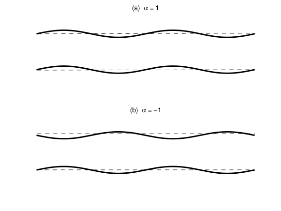
Figure 1: (a) bending waves; (b) contraction/expansion waves.

The results of numerical solution of the Navier-Stokes equations subject to the boundary conditions (5.4) are shown in Fig. 2. Qualitatively, the stream line picture is the same for both bending and contraction/expansion waves. The magnitudes of the averaged flow in these two cases are different for $L_{x}>1$. Let us measure the magnitude of the velocity field by $\max|\bar{{\bf v}}_{1}^{r}|$ where the maximum is computed for all $(x,z)$ such that $0\leq x\leq L_{x}$, $0\leq z\leq 1$. Table 1 shows $\max|\bar{{\bf v}}_{1}^{r}|$ for various $L_{x}$. Evidently, the maximum velocity decreases, when wavelength $L_{x}$ increases, much faster for bending waves ($\alpha=1$) than for contraction/expansion waves ($\alpha=-1$).

$L_{x}$		0.5	1	5
$\max|\bar{{\bf v}}_{1}^{r}|$	$\alpha=1$	2.3562	1.1693	0.073073
	$\alpha=-1$	2.3562	1.1869	0.75974

Table 1: $\max|\bar{{\bf v}}_{1}^{r}|$ for standing waves and $\nu=1$.

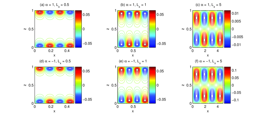
Figure 2: Streamlines of the averaged velocity for $\nu=1$ (standing waves).

5.2 Example 2: travelling waves

Consider now vibrations of the walls in the form of plane travelling waves:

$$f({\bf r},\tau)=\cos(kx-\tau),\quad g({\bf r},\tau)=\alpha\cos(kx-\beta\tau),$$ (5.5)

where $k=2\pi/L_{x}$, $\alpha=\pm 1$ and $\beta=\pm 1$. If $\beta=1$, both waves travel in the same direction, if $\beta=-1$, the waves travel in opposite directions. Since both $f$ and $g$ do not depend on $y$, we will look for a solution which does not depend on $y$. Problem (3.5) simplifies to

$$\phi_{0xx}+\phi_{0zz}=0,\quad\phi_{0}(x+L_{x},z)=\phi_{0}(x,z),$$

$$\phi_{0z}\!\bigm{|}_{z=0}=\sin(kx-\tau),\quad\phi_{0z}\!\bigm{|}_{z=1}=\alpha\sin(kx-\tau).$$ (5.6)

Consider first $\beta=1$, i.e. both waves travel in the positive direction of the $x$ axis. Boundary conditions (4.24)–(4.27) become

$$\bar{u}_{1}^{r}\!\bigm{|}_{z=0}=A(k),\quad\bar{u}_{1}^{r}\!\bigm{|}_{z=1}=A(k),\quad\bar{w}_{1}^{r}\!\bigm{|}_{z=0}=0,\quad\bar{w}_{1}^{r}\!\bigm{|}_{z=1}=0,$$ (5.7)

where

$$A(k)=\frac{k}{4\sinh^{2}(k)}\left[5+\cosh^{2}(k)-6\alpha\cosh(k)\right]$$

The Stokes drift velocity is given by

$${\bf V}({\bf r})=V_{0}(z){\bf e}_{x},\quad V_{0}(z)=\frac{k\left[\cosh(k)-\alpha\right]}{\sinh^{2}(k)}\cosh\left[k(2z-1)\right].$$ (5.8)

Now $\bar{\boldsymbol{\omega}}_{1}^{r}=\Omega(x,z){\bf e}_{y}$ where $\Omega(x,z)={\partial}_{z}\bar{u}_{1}^{r}-{\partial}_{x}\bar{w}_{1}^{r}$, and Eq. (3.21) can be written as

$$(\bar{{\bf v}}^{r}_{1}\cdot\nabla)\bar{{\bf v}}^{r}_{1}=-\nabla\Pi_{3}+\nu\nabla^{2}\bar{{\bf v}}^{r}_{1}+V_{0}(z)\Omega\,{\bf e}_{z}.$$ (5.9)

Equation (5.9) subject to boundary conditions (5.7) has the constant solution

$$\bar{{\bf v}}_{1}^{r}=A(k){\bf e}_{x}.$$ (5.10)

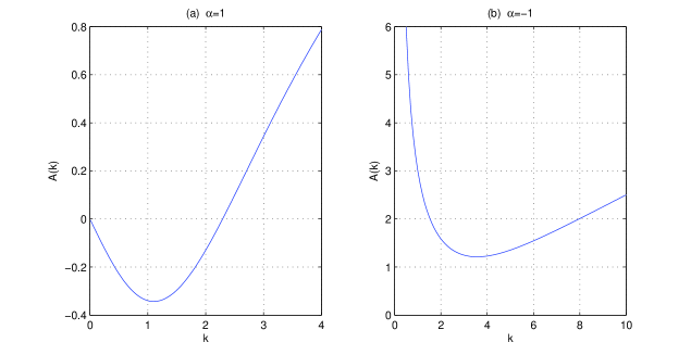
Figure 3: The averaged Eulerian velocity as function of $k$.

The constant horizontal velocity as function of $k$ is shown in Fig. 3. For bending waves, it is negative for small $k$ and positive for large $k$ ($A(k)\sim k$ for both $k\ll 1$ and $k\gg 1$). For contraction/expansion waves, it is always positive and growing both when $k\to 0$ and when $k\to\infty$ ($A(k)\sim 1/k$ for $k\ll 1$ and $A(k)\sim k$ for $k\gg 1$).

Although Eq. (5.9) also has solutions with a nonzero pressure gradient $\nabla\Pi_{3}=c_{0}{\bf e}_{x}$ ($c_{0}=const$), we do not consider such solutions here, because this would amount to a modification of our original problem, allowing the presence of a weak $O({\epsilon}^{3})$ pressure gradient. Note also that flows with stronger pressure gradients would require a separate treatment.

The averaged Lagrangian velocity is given by

$$\bar{{\bf v}}_{1}^{L}=\bar{{\bf v}}_{1}^{r}+{\bf V}=V^{L}(z){\bf e}_{x},\quad V^{L}(z)=A(k)+V_{0}(z).$$

Its profiles for various values of $k$ are shown in Fig. 4. In the short wave limit, $V^{L}(z)$ is constant almost everywhere except narrow layers near the boundary where the velocity is much higher (see Fig. 5). This can also be seen from the asymptotic formula

$$V^{L}=k\left(\frac{1}{4}+e^{-2kz}+e^{-2k(1-z)}\right)+O(ke^{-k}),\quad k\to\infty.$$

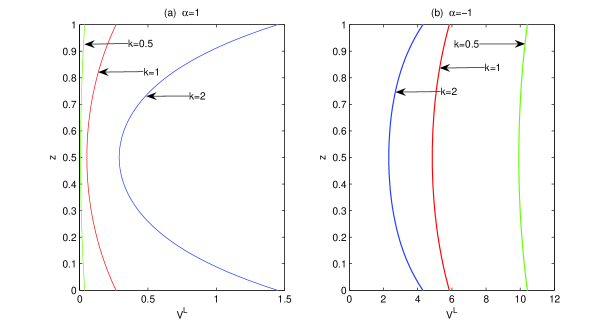
Figure 4: The averaged Lagrangian velocity profiles for $\beta=1$ (waves travelling in the same direction).

Now let $\beta=-1$. In this case, boundary conditions (4.24)–(4.27) take the form

$$\bar{u}_{1}^{r}\!\bigm{|}_{z=0}=B^{+}(k,x),\quad\bar{u}_{1}^{r}\!\bigm{|}_{z=1}=B^{-}(k,x),\quad\bar{w}_{1}^{r}\!\bigm{|}_{z=0}=C(k,x),\quad\bar{w}_{1}^{r}\!\bigm{|}_{z=1}=C(k,x),$$ (5.11)

where

$$B^{\pm}(k,x)=\frac{k}{4}\left[\pm 1+6\alpha\frac{\cosh(k)}{\sinh^{2}(k)}\sin(2kx)\right],\quad C(k,x)=\alpha\frac{k\sin(2kx)}{\sinh(k)}.$$ (5.12)

Thus in the case of waves travelling in opposite directions, we have nonzero boundary conditions for the normal velocity in the averaged outer flow.

The Stokes drift velocity is given by

$${\bf V}({\bf r})=V_{1}(z){\bf e}_{x}+V_{3}(x){\bf e}_{z},\quad V_{1}(z)=-k\frac{\sinh[k(2z-1)]}{\sinh(k)},\quad V_{3}(z)=-C(k,x),$$ (5.13)

where $C(k,x)$ is given by (5.12). Note that Eq. (5.13) implies that the normal component of the averaged Lagrangian velocity at the walls is zero: $w^{L}=\bar{w}_{1}^{r}+V_{3}=0$ at $z=0$ and $z=1$, which is in agreement with the general property discussed in Appendix A.

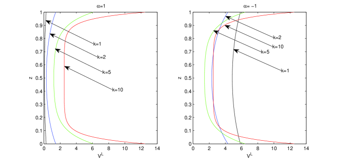
Figure 5: The averaged Lagrangian velocity profiles for $\beta=1$ (waves travelling in the same direction) and $k\geq 1$ (short waves).

Further, we have $\hat{\boldsymbol{\omega}}_{1}^{r}=\Omega(x,z)\,{\bf e}_{y}$ where, as before, $\Omega(x,z)={\partial}_{z}u_{1}^{r}-{\partial}_{x}w_{1}^{r}$, and Eq. (3.21) can be written as

$$(\bar{{\bf v}}^{r}_{1}\cdot\nabla)\bar{{\bf v}}^{r}_{1}=-\nabla\Pi_{3}+\nu\nabla^{2}\bar{{\bf v}}^{r}_{1}+\Omega\left[V_{1}(z)\,{\bf e}_{z}-V_{3}(x)\,{\bf e}_{x}\right].$$ (5.14)

Thus, the averaged Eulerian velocity can be found by solving Eq. (5.14) subject to boundary conditions (5.11). Then the averaged Lagrangian velocity is obtained by adding the Stokes drift velocity given by Eq. (5.13).

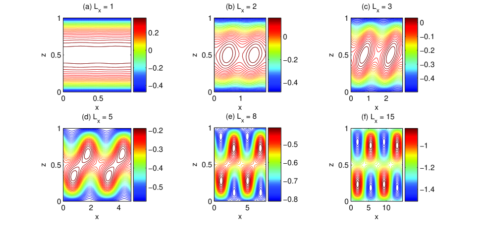
Figure 6: Streamlines of the averaged Lagrangian velocity for $\alpha=1$ and $\nu=1$ (waves travelling in opposite directions).

Equation (5.14) supplemented with the incompressibility condition and boundary conditions (5.11) were solved numerically. The streamlines of the averaged Lagrangian velocity ${\bf v}^{L}$ for $\alpha=1$ and $\nu=1$ are shown in Fig. 6. The corresponding values of $\max|\bar{{\bf v}}_{1}^{r}|$ are given in Table 2. In the case $\alpha=-1$, the same flow pattern is shifted by a quarter of the wavelength in the $x$ direction.

$L_{x}$	1	2	3	5	8	15
$\max|\bar{{\bf v}}_{1}^{r}|$	0.80301	0.60373	0.71208	1.0467	1.6146	2.9929

Table 2: $\max|\bar{{\bf v}}_{1}^{r}|$ for $\beta=-1$, $\alpha=1$ and $\nu=1$ (waves travelling in opposite directions).

5.3 General periodic vibrations

Here we will briefly describe how to treat the case of general periodic (both in time and space) transverse vibrations of the wall. We focus our attention on the travelling waves for which we will present an explicit solution.

Let $\boldsymbol{\sigma}$ be the projection of $\boldsymbol{\zeta}$ (defined by Eq. (3.18)) onto the $xy$ plane, i.e.

$$\boldsymbol{\sigma}=\boldsymbol{\zeta}-(\boldsymbol{\zeta}\cdot{\bf e}_{z}){\bf e}_{z},$$ (5.15)

and let

$$\boldsymbol{\sigma}^{a}=\boldsymbol{\sigma}\!\bigm{|}_{z=0},\quad\boldsymbol{\sigma}^{b}=\boldsymbol{\sigma}\!\bigm{|}_{z=1}.$$ (5.16)

Let us express boundary conditions (4.24), (4.25) in terms of $f$, $g$, $\boldsymbol{\sigma}^{a}$ and $\boldsymbol{\sigma}^{b}$.

First, we note that since $\boldsymbol{\sigma}^{a}$ and $\boldsymbol{\sigma}^{b}$ are periodic functions of $\tau$ with period $2\pi$, they can be written as Fourier series

$$\boldsymbol{\sigma}=\sum_{n}\hat{\boldsymbol{\sigma}}_{n}({\bf r},z)e^{in\tau},\quad\boldsymbol{\sigma}^{a}=\sum_{n}\hat{\boldsymbol{\sigma}}^{a}_{n}({\bf r})e^{in\tau},\quad\boldsymbol{\sigma}^{b}=\sum_{n}\hat{\boldsymbol{\sigma}}^{b}_{n}({\bf r})e^{in\tau}.$$ (5.17)

Here and in what follows (unless explicitly specified otherwise) summation is performed over all integers. Also, in Eq. (5.17),

$$\hat{\boldsymbol{\sigma}}_{0}({\bf r},z)\equiv 0,\quad\hat{\boldsymbol{\sigma}}^{a}_{0}({\bf r})\equiv 0,\quad\hat{\boldsymbol{\sigma}}^{b}_{0}({\bf r})\equiv 0.$$

Now boundary conditions (4.3) and (4.9) can be written as

$${\bf U}^{a}_{0}\!\bigm{|}_{s=0}=-i\sum_{n}n\hat{\boldsymbol{\sigma}}^{a}_{n}e^{in\tau},\quad{\bf U}^{b}_{0}\!\bigm{|}_{q=0}=-i\sum_{n}n\hat{\boldsymbol{\sigma}}^{b}_{n}e^{in\tau}.$$ (5.18)

Periodic solutions of Eqs. (4.2) and (4.8) subject to boundary conditions (5.18) and the condition of decay at infinity (in $s$ and $q$ respectively) are given by

$${\bf U}^{a}_{0}=-i\sum_{n}n\hat{\boldsymbol{\sigma}}^{a}_{n}e^{in\tau-\mu_{n}s},\quad{\bf U}^{b}_{0}=-i\sum_{n}n\hat{\boldsymbol{\sigma}}^{b}_{n}e^{in\tau-\mu_{n}q},$$ (5.19)

where

$$\mu_{n}=\sqrt{\frac{|n|}{2\nu}}(1+i\,\mathrm{sgn}(n)).$$ (5.20)

It is shown in Appendix B that boundary conditions for $\bar{{\bf u}}_{1}^{r}$ (given by (4.24) and (4.25)) can be written as

$$\bar{{\bf u}}^{r}_{1}\!\bigm{|}_{z=0}=\overline{f_{\tau}\,\boldsymbol{\sigma}_{z}}\!\bigm{|}_{z=0}-\frac{3}{2}\overline{\boldsymbol{\sigma}^{a}_{\tau}(\nabla_{\parallel}\cdot\boldsymbol{\sigma}^{a})}-\frac{1}{4}\nabla_{\parallel}\left(\sum_{n}|n||\hat{\boldsymbol{\sigma}}^{a}_{n}|^{2}\right)-\sum_{n}|n|\,\mathrm{Re}\left[\hat{\boldsymbol{\sigma}}^{a*}_{n}(\nabla_{\parallel}\cdot\hat{\boldsymbol{\sigma}}^{a}_{n})\right],\qquad\quad$$ (5.21)

$$\bar{{\bf u}}^{r}_{1}\!\bigm{|}_{z=1}=\overline{g_{\tau}\,\boldsymbol{\sigma}_{z}}\!\bigm{|}_{z=1}-\frac{3}{2}\overline{\boldsymbol{\sigma}^{b}_{\tau}(\nabla_{\parallel}\cdot\boldsymbol{\sigma}^{b})}-\frac{1}{4}\nabla_{\parallel}\left(\sum_{n}|n||\hat{\boldsymbol{\sigma}}^{b}_{n}|^{2}\right)-\sum_{n}|n|\,\mathrm{Re}\left[\hat{\boldsymbol{\sigma}}^{b*}_{n}(\nabla_{\parallel}\cdot\hat{\boldsymbol{\sigma}}^{b}_{n})\right].\qquad\quad$$ (5.22)

From now on we will restrict our analysis to the two-dimensional case, where both $f$ and $g$ do not depend on $y$ and ${{\bf u}}^{r}_{1}=u^{r}_{1}{\bf e}_{x}$, ${\boldsymbol{\sigma}}=\sigma{\bf e}_{x}$. Equations (5.21) and (5.22) simplify to

$$\bar{u}^{r}_{1}\!\bigm{|}_{z=0}=\overline{f_{\tau}\,\sigma_{z}}\!\bigm{|}_{z=0}-\frac{3}{2}\,\overline{\sigma^{a}_{\tau}\sigma^{a}_{x}}-\frac{3}{4}\,\partial_{x}\left(\sum_{n}|n||\hat{\sigma}^{a}_{n}|^{2}\right),\qquad\quad$$ (5.23)

$$\bar{u}^{r}_{1}\!\bigm{|}_{z=1}=\overline{g_{\tau}\,\sigma_{z}}\!\bigm{|}_{z=1}-\frac{3}{2}\,\overline{\sigma^{b}_{\tau}\sigma^{b}_{x}}-\frac{3}{4}\,\partial_{x}\left(\sum_{n}|n||\hat{\sigma}^{b}_{n}|^{2}\right).\qquad\quad$$ (5.24)

For simplicity, we consider only vibrations of the walls in the form of plane waves of arbitrary shape travelling in the same direction, namely, we assume that

$$f(x,\tau)=F(kx-\tau),\quad g(x,\tau)=\alpha F(kx-\tau),$$ (5.25)

where $F$ is an arbitrary $2\pi$-periodic function of a single variable $h=kx-\tau$; $k$ and $\alpha$ are the same as those defined in Section 5.2. Let $\hat{F}_{n}$ be the Fourier coefficients of $F$. Then the solution of problem (3.5) is

$$\phi_{0}(z,h)=\sum_{n}inb_{n}(z)\hat{F}_{n}e^{inh}$$ (5.26)

where

$$b_{n}(z)=\frac{\cosh[|kn|(1-z)]-\alpha\cosh[|kn|z]}{|kn|\sinh|kn|}.$$

Further, we have

$$\sigma(z,h)=-ik\sum_{n}nb_{n}(z)\hat{F}_{n}e^{inh}$$ (5.27)

and

$$\sigma^{a}(h)=i\alpha k\sum_{n}nQ_{n}\hat{F}_{n}e^{inh},\quad\sigma^{b}(h)=-ik\sum_{n}nQ_{n}\hat{F}_{n}e^{inh},\quad Q_{n}\equiv\frac{1-\alpha\cosh|kn|}{|kn|\sinh|kn|}.$$ (5.28)

It follows from (5.28) that

$$\hat{\sigma}^{a}_{-n}(x)=ikn\alpha Q_{n}\hat{F}_{n}e^{inkx},\quad\hat{\sigma}^{b}_{-n}(x)=-iknQ_{n}\hat{F}_{n}e^{inkx}.$$ (5.29)

Substitution of (5.27)–(5.29) into (5.23), (5.24) and tedious but elementary calculations yield (cf. Eq. (5.7))

$$\bar{u}^{r}_{1}\!\bigm{|}_{z=0}=\bar{u}^{r}_{1}\!\bigm{|}_{z=1}=A(k),$$

$$A(k)=k\sum_{n}n^{2}|\hat{F}_{n}|^{2}\frac{5+\cosh^{2}|kn|-6\alpha\cosh|kn|}{2\sinh^{2}|kn|}$$

$$\quad\quad\ =k\sum_{n=1}^{\infty}n^{2}|\hat{F}_{n}|^{2}\frac{5+\cosh^{2}(kn)-6\alpha\cosh(kn)}{\sinh^{2}(kn)}.$$ (5.30)

Boundary conditions for $\bar{w}_{1}^{r}$ (given by (4.26), (4.27)) reduce to

$$\bar{w}_{1}^{r}\!\bigm{|}_{z=0}=0,\quad\bar{w}_{1}^{r}\!\bigm{|}_{z=1}=0.$$ (5.31)

Similar calculations of the Stokes drift velocity yield

$${\bf V}=V_{0}(z){\bf e}_{x}$$

where (cf. Eq. (5.8))

$$V_{0} = 2k\sum_{n}n^{2}|\hat{F}_{n}|^{2}\frac{\cosh|kn|-\alpha}{\sinh^{2}|kn|}\,\cosh\left[|kn|(2z-1)\right]$$ (5.32)

$$= 4k\sum_{n=1}^{\infty}n^{2}|\hat{F}_{n}|^{2}\frac{\cosh(kn)-\alpha}{\sinh^{2}(kn)}\,\cosh\left[kn(2z-1)\right].$$

Boundary conditions (5.30) and (5.31) results in a constant solution of Eq. (5.9): ${\bf v}_{1}^{r}=A(k){\bf e}_{x}$, which is a generalisation of the solution (5.10) obtained in Section 5.2. The averaged Lagrangian velocity is

$${\bf V}^{L}=V^{L}{\bf e}_{x},\quad V^{L}\equiv A+V_{0}(z).$$

Let us compute the total volume flux of the fluid through the channel (per unit length in $y$ direction). We have

$$Q=\int_{0}^{1}V^{L}\,dz=A+\int_{0}^{1}V_{0}(z)\,dz=\sum_{n=1}^{\infty}n^{2}|\hat{F}_{n}|^{2}\,R_{n}(k)$$ (5.33)

where

$$R_{n}=\frac{k}{\sinh^{2}(kn)}\left(5+\cosh^{2}(kn)-6\alpha\cosh(kn)+4\left[\cosh(kn)-\alpha\right]\,\frac{\sinh(kn)}{kn}\right).$$ (5.34)

Optimal shape of the wave. Now we can answer the question on what shape of the travelling waves leads to the the most efficient generation of the averaged flow. Mathematically, this can formulated as the following optimization problem: maximize the total volume flux $Q$ on the set of all $\hat{F}_{n}$ such that

$$\sum_{n=1}^{\infty}n^{2}|\hat{F}_{n}|^{2}=1.$$ (5.35)

Let $m\in\mathbb{N}$ be such that

$$R_{m}=\max_{n\in\mathbb{N}}R_{n}.$$ (5.36)

It is not difficult to show that $Q$ attains its maximum for

$$\hat{F}_{n}=\frac{e^{i\lambda}}{|n|}\,\delta_{|n\!|m}\quad(n=\pm 1,\pm 2,\dots),$$

where $\lambda$ is any real number. For contraction/expansion waves ($\alpha=-1$), the sequence $\{R_{n}\}$ is monotonically decreasing for all $k>0$, so that the maximum is attained at $n=1$. Thus, the most efficient deformation of the walls is given by (cf. (5.6))

$$f(x,\tau)=2\cos(kx-\tau+\lambda),\quad g(x,\tau)=-f(x,\tau).$$

In the case of bending waves, the mode for which the maximum total flux is attained depends on $k$ as shown in Fig. 7. One can see that $m$ is equal to 1 for $k\gtrsim 2.9$ (i.e. for sufficiently short waves) and increases when $k$ decreases. The most efficient deformation has the form:

$$f(x,\tau)=g(x,\tau)=2\cos[m(kx-\tau)+\lambda]/m.$$

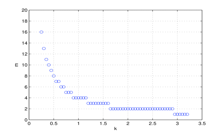
Figure 7: $m$, defined by (5.36), as a function of $k$ for bending waves ($\alpha=1$).

6 Discussion

We have considered incompressible flows between two transversely vibrating solid walls and proposed a general procedure for constructing an asymptotic expansion of solutions of the Navier-Stokes equations in the limit when both the amplitude of vibrations and the thickness of the Stokes layer are small and have the same order of magnitude. The procedure is based on the Vishik-Lyusternik method and, in principle, can be used to construct as many terms of the expansion as necessary. In the leading order, the averaged flow is described by the stationary Navier-Stokes equations with an additional term which contains the leading-order Stokes drift velocity. In a slightly different context (for a flow induced by an oscillating conservative body force), the same equations had been derived earlier by Riley [3].

The general theory has been applied to two particular examples of steady streaming induced by vibrations of the walls in the form of standing and travelling plane waves. In the case of plane standing waves (bending or contraction/expansion waves), the averaged flow has the form of a double array of vortices (see Fig. 2). For short waves the vortices are concentrated near the walls, while long waves produce vortices that fill the entire channel. The latter pattern is similar to flows produced by long standing waves at small Reynolds numbers [6]. For both bending and contraction/expansion waves, the flow patterns are qualitatively the same. However, the intensity of the averaged flow is different. Although it is of similar magnitude for both waves when the wavelength is small, for long waves, the maximum velocity decreases much faster for bending waves than for contraction/expansion waves, which is in agreement with the classical theory of peristaltic pumping at low Reynolds numbers (see, e.g., [15]).

If vibrations of the wall have the form of plane harmonic waves which travel in the same direction (this leads to a bending wave if the phase shift between these travelling waves is zero, and to a contraction/expansion wave if the phase shift is $\pi$), the induced steady flow is a unidirectional two-dimensional flow. The fortunate thing is that, in this case, the asymptotic equations can be solved analytically. The Lagrangian velocity profile is symmetric relative to the channel central axis, with a minimum velocity at the centre and maxima at the walls. In the short wave limit, the Lagrangian velocity profiles for both bending and contraction/expansion waves are the same: the velocity is nearly constant across the channel except for narrow layers near the walls where velocity is much higher. For moderate and long waves, the velocity variation across the channel is much smaller, and the magnitude of the velocity rapidly grows for the contraction/expansion wave and decays for the bending wave when the wavelength increases. This example may be viewed as an extension of the theory of peristaltic pumping to the case of high Reynolds numbers.

If vibrations of the walls have the form of plane harmonic waves traveling in opposite directions, the averaged flow depends on the wavelength in a more complicated way. For short waves the averaged flow is a superposition of a shear flow with a linear velocity profile and a periodic array of weak vortices (‘cat’s eyes’) in the center of the channel. When the wavelength increases, the vortices first grow in size and magnitude. Then each of them splits into a pair of vortices of the same sign, and at the same time new vortices appear near the walls and move towards the centre of the channel. Eventually, for long waves, there are two arrays of alternating vortices (similar to what we had in the case of standing waves).

As an example of general periodic vibrations, we have considered travelling contraction/expansion and bending waves of an arbitrary shape. Similarly to the case of a harmonic vibration, these produce unidirectional two-dimensional flows. The averaged Lagrangian velocity is written as an infinite series in term of Fourier coefficients of the deformations of the walls. The natural question that appears here is: what deformations of the walls lead to a maximum total volume flux through the channel. It turns out that the optimal shape always corresponds to a single harmonic. For a contraction/expansion wave, it is always the first harmonic (with $m=1$). For a bending wave, the optimal harmonic is uniquely determined by the parameter $k=2\pi/L_{x}$. For example, if $k=1$, then $m=4$. It should be noted here that a contraction/expansion wave always produces a higher total volume flux then a bending wave.

There are many open problems in this area. First, it is not quite clear how the present theory can be extended to the case of high $R_{s}$. Second, we did not make any assumption about the characteristic length scale of vibrations in the horizontal direction. Nevertheless, the examples show that the theory does not work when the horizontal length scale is much smaller than the mean distance between the walls. In particular, Figures 2 and 5 shows that for $L_{x}<1$ the flows in Examples 1 and 2 become concentrated near the walls. This suggests that in the limit of short waves, one can try to construct a theory with double boundary layers (similar to what had been done by Stuart [8] and Riley [9] for an oscillating cylinder at $R_{s}\gg 1$). Third, it would be interesting to investigate the effect of an external mean flow (e.g., a flow produced by a mean pressure gradient) on the steady steaming between two walls and vice versa. This problem has an additional parameter - the ratio of the characteristic velocity of the mean flow to the amplitude of the velocity of the vibrating walls and, therefore, one can expect a variety of different flow regimes. All these are problems for a future investigation.

Acknowledgments. This work was initiated during a short visit of Andrey Morgulis to the University of York under the University of York Research Development Visit scheme.

7 Appendix A

Here we will show that

$$V_{3}\!\bigm{|}_{z=0}=-\nabla_{\|}\cdot\overline{(f\nabla_{\|}\phi_{0})}\!\bigm{|}_{z=0},\quad V_{3}\!\bigm{|}_{z=1}=-\nabla_{\|}\cdot\overline{(g\nabla_{\|}\phi_{0})}\!\bigm{|}_{z=1},$$ (A.1)

where $V_{3}$ is the z-component of the Stokes drift velocity ${\bf V}$ given by Eq. (3.22).

We have

$$V_{3} = {\bf V}\cdot{\bf e}_{z}=\frac{1}{2}{\bf e}_{z}\cdot\overline{\left[\boldsymbol{\zeta}_{\tau},\boldsymbol{\zeta}\right]}=-\overline{(\boldsymbol{\zeta}_{\tau}\cdot\nabla)(\boldsymbol{\zeta}\cdot{\bf e}_{z})}=-\nabla\cdot\overline{[\boldsymbol{\zeta}_{\tau}(\boldsymbol{\zeta}\cdot{\bf e}_{z})]}$$ (A.2)

$$= -{\partial}_{z}\overline{[(\boldsymbol{\zeta}_{\tau}\cdot{\bf e}_{z})(\boldsymbol{\zeta}\cdot{\bf e}_{z})]}-\nabla_{\|}\cdot\overline{[{\bf u}_{0}^{r}(\boldsymbol{\zeta}\cdot{\bf e}_{z})]}=-\nabla_{\|}\cdot\overline{[{\bf u}_{0}^{r}(\boldsymbol{\zeta}\cdot{\bf e}_{z})]}.$$

It follows from (3.18) and (3.5) that $\boldsymbol{\zeta}\cdot{\bf e}_{z}|_{z=0}=f$ and $\boldsymbol{\zeta}\cdot{\bf e}_{z}|_{z=1}=g$. These and (A.2) imply the relations

$$V_{3}\!\bigm{|}_{z=0}=-\nabla_{\|}\cdot\overline{(f{\bf u}_{0}^{r})}\!\bigm{|}_{z=0}\quad{\rm and}\quad V_{3}\!\bigm{|}_{z=1}=-\nabla_{\|}\cdot\overline{(g{\bf u}_{0}^{r})}\!\bigm{|}_{z=0}$$

that are equivalent to (A.1).

8 Appendix B

Here we will briefly describe the derivation of Eq. (5.21). Equation (5.22) can be derived in exactly the same way.

First, we use (4.9) and (4.11) to rewrite Eq. (4.16) as

$${\bf H}^{a}_{1} = \left(s\nabla_{\parallel}^{2}\phi_{0}^{0}+W_{0}^{a}\!\bigm{|}_{s=0}-W_{0}^{a}+({\bf U}_{0}^{a}-{\bf U}_{0}^{a}\!\bigm{|}_{s=0})\cdot\nabla_{\parallel}f\right){\bf U}^{a}_{0s}$$ (B.1)

$$-({\bf U}_{0}^{a}\cdot\nabla_{\parallel}){\bf U}_{0}^{a}-(\nabla_{\parallel}\phi_{0}^{0}\cdot\nabla_{\parallel}){\bf U}_{0}^{a}-({\bf U}_{0}^{a}\cdot\nabla_{\parallel})\nabla_{\parallel}\phi_{0}^{0}.$$

Here $\phi_{0}^{0}=\phi_{0}\!\bigm{|}_{z=0}$. With the help of (4.5), this can be further simplified to

$${\bf H}^{a}_{1} = \left(s\nabla_{\parallel}^{2}\phi_{0}^{0}+\nabla_{\parallel}\cdot\int\limits_{0}^{s}{\bf U}^{a}_{0}(s^{\prime})ds^{\prime}\right){\bf U}^{a}_{0s}$$ (B.2)

$$-({\bf U}_{0}^{a}\cdot\nabla_{\parallel}){\bf U}_{0}^{a}-(\nabla_{\parallel}\phi_{0}^{0}\cdot\nabla_{\parallel}){\bf U}_{0}^{a}-({\bf U}_{0}^{a}\cdot\nabla_{\parallel})\nabla_{\parallel}\phi_{0}^{0}.$$

Equation (4.2), (4.3) and the fact that ${\bf u}_{0}^{r}=\nabla_{\parallel}\phi_{0}$ imply that ${\bf e}_{z}\cdot\mathrm{curl}{\bf U}_{0}^{a}=0$. Therefore, (B.2) can be rewritten as

$${\bf H}^{a}_{1}=\left(s\nabla_{\parallel}^{2}\phi_{0}^{0}+\nabla_{\parallel}\cdot\int\limits_{0}^{s}{\bf U}^{a}_{0}(s^{\prime})ds^{\prime}\right){\bf U}^{a}_{0s}-\nabla_{\parallel}\left(\frac{{\bf U}^{a2}_{0}}{2}+{\bf U}^{a}_{0}\cdot\nabla_{\parallel}\phi_{0}^{0}\right).$$ (B.3)

It follows from (4.18) that

$$\bar{{\bf U}}^{a}_{1}\!\bigm{|}_{s=0}=-\frac{1}{\nu}\int\limits_{0}^{\infty}\int\limits_{s^{\prime}}^{\infty}\bar{{\bf H}}_{1}^{a}(s^{\prime\prime})\,ds^{\prime\prime}\,ds^{\prime}=-\frac{1}{\nu}\int\limits_{0}^{\infty}\bar{{\bf H}}_{1}^{a}(s^{\prime\prime})\int\limits_{0}^{s^{\prime\prime}}\,ds^{\prime}\,ds^{\prime\prime}=-\frac{1}{\nu}\int\limits_{0}^{\infty}s^{\prime\prime}\,\bar{{\bf H}}_{1}^{a}(s^{\prime\prime})\,ds^{\prime\prime}.$$ (B.4)

On substituting (B.3) into (B.4), we obtain

$$\bar{{\bf U}}^{a}_{1}\!\bigm{|}_{s=0} = \frac{2}{\nu}\,\overline{\nabla_{\parallel}^{2}\phi_{0}^{0}\int\limits_{0}^{\infty}s\,{\bf U}^{a}_{0}\,ds}+\frac{1}{\nu}\nabla_{\parallel}\int\limits_{0}^{\infty}\left(\overline{\frac{({\bf U}^{a}_{0})^{2}}{2}}+\overline{{\bf U}^{a}_{0}\cdot\nabla_{\parallel}\phi_{0}^{0}}\right)s\,ds$$ (B.5)

$$-\frac{1}{\nu}\overline{\int\limits_{0}^{\infty}s\,{\bf U}^{a}_{0s}(s)\left(\nabla_{\parallel}\cdot\int\limits_{0}^{s}{\bf U}^{a}_{0}(s^{\prime})\,ds^{\prime}\right)ds}.$$

It follows from (5.19) that

$$\int\limits_{0}^{\infty}s\,{\bf U}^{a}_{0}\,ds=-i\sum_{n}n\,\hat{\boldsymbol{\sigma}}_{n}^{a}e^{in\tau}\int\limits_{0}^{\infty}s\,e^{-\mu_{n}s}\,ds=-i\sum_{n}n\,\hat{\boldsymbol{\sigma}}_{n}^{a}\frac{1}{\mu_{n}^{2}}\,e^{in\tau}=-\nu\sum_{n}\hat{\boldsymbol{\sigma}}_{n}^{a}\,e^{in\tau}=-\nu\boldsymbol{\sigma}^{a}.$$

Hence,

$$\frac{2}{\nu}\,\overline{\nabla_{\parallel}^{2}\phi_{0}^{0}\int\limits_{0}^{\infty}s\,{\bf U}^{a}_{0}\,ds}=-2\,\overline{\left(\nabla_{\parallel}\cdot\boldsymbol{\sigma}^{a}_{\tau}\right)\boldsymbol{\sigma}^{a}}=2\,\overline{\left(\nabla_{\parallel}\cdot\boldsymbol{\sigma}^{a}\right)\boldsymbol{\sigma}^{a}_{\tau}}.$$ (B.6)

Similar calculations yield

$$\int\limits_{0}^{\infty}\overline{\frac{({\bf U}^{a}_{0})^{2}}{2}}\,s\,ds=\frac{\nu}{4}\sum_{n}|n||\hat{\boldsymbol{\sigma}}^{a}_{n}|^{2},\quad\overline{\nabla_{\parallel}\phi_{0}^{0}\cdot\int\limits_{0}^{\infty}{\bf U}^{a}_{0}\,s\,ds}=-2\nu\,\overline{\boldsymbol{\sigma}^{a}_{\tau}\cdot\boldsymbol{\sigma}^{a}}=0,$$ (B.7)

$$\overline{\int\limits_{0}^{\infty}s\,{\bf U}^{a}_{0s}(s)\left(\nabla_{\parallel}\cdot\int\limits_{0}^{s}{\bf U}^{a}_{0}(s^{\prime})\,ds^{\prime}\right)ds}=\nu\sum_{n}|n|\,\mathrm{Re}\left[\hat{\boldsymbol{\sigma}}^{a*}_{n}\left(\nabla_{\parallel}\cdot\hat{\boldsymbol{\sigma}}^{a}_{n}\right)\right]-\frac{\nu}{2}\,\overline{\left(\nabla_{\parallel}\cdot\boldsymbol{\sigma}^{a}\right)\boldsymbol{\sigma}^{a}_{\tau}}.\qquad$$ (B.8)

Substituting (B.6)–(B.9) into (B.5), we find that

$$\bar{{\bf U}}^{a}_{1}\!\bigm{|}_{s=0}=\frac{3}{2}\,\overline{\left(\nabla_{\parallel}\cdot\boldsymbol{\sigma}^{a}\right)\boldsymbol{\sigma}^{a}_{\tau}}+\frac{1}{4}\sum_{n}|n||\hat{\boldsymbol{\sigma}}^{a}_{n}|^{2}+\sum_{n}|n|\,\mathrm{Re}\left[\hat{\boldsymbol{\sigma}}^{a*}_{n}\left(\nabla_{\parallel}\cdot\hat{\boldsymbol{\sigma}}^{a}_{n}\right)\right].$$ (B.9)

Finally, substitution of (B.9) into (4.24) results in boundary condition (5.21).

References

- [1] Lighthill, J. 1978 Acoustic Streaming. J. Sound and Vibration, 61(3), 391 418.
- [2] Riley, N. 1967 Oscillatory Viscous Flows. Review and Extension. J. Inst. Maths Applics, 3, 419–434.
- [3] Riley, N. 2001 Steady Streaming. Ann. Rev. Fluid Mech., 33, 43 65.
- [4] Selverov, J. P. & Stone, H. A. 2001 Peristaltically driven channel flows with applications towards micromixing. Phys. Fluids, 13(7), 1838–1859.
- [5] Yi, M., Bau, H. H. & Hu, H. 2002 Peristaltically induced motion in a closed cavity with two vibrating walls. Phys. Fluids, 14(1), 184–197.
- [6] Carlsson, F. , Sen. M. & Löfdahl, H. A. 2005 Fluid mixing induced by vibrating walls. European J. Mech. B/Fluids, 24, 366–378.
- [7] Hœpffner, J. & Fukagata, K. 2009 Pumping or drag reduction? J. Fluid Mech., 635, 171–187.
- [8] Stuart, J. T. 1966 Double boundary layers in oscillatory viscous flow. J. Fluid Mech., 42(4), 673–687.
- [9] Riley, N. 1965 Oscillating viscous flows. Mathematika, 12, 161–175.
- [10] Wang, Ch.-Y. 1968 On high-frequency oscillatory viscous flows. J. Fluid Mech., 32(1), 55–68.
- [11] Bertelsen, A., Svardal, A. & Tjtta, S. 1973 Nonlinear streaming effects associated with oscillating cylinders. J. Fluid Mech., 59(3), 493–511.
- [12] Riley, N. 1975 The steady streaming induced by a vibrating cylinder. J. Fluid Mech., 68, 801–812.
- [13] Haddon, E. W. & Riley, N. 1979 The steady streaming induced between oscillating circular cylinders. Q. J. Mech. Appl. Math., 32(3), 801–812.
- [14] Duck, P. W. & Smith, F. T. 1979 Steady streaming induced between oscillating cylinders. J. Fluid Mech., 91, 93–110.
- [15] Jaffrin, M. Y. & Shapiro, A. H. 1971 Peristaltic pumping. Ann. Rev. Fluid Mech., 3, 13 37.
- [16] Wilson,D. E. & Panton, R. L. 1979 Peristaltic transport due to finite amplitude bending and contraction waves. J. Fluid Mech., 90, 145–159.
- [17] Longuet-Higgens, M. S. 1953 Mass transport in water waves. Philos. Trans. Roy. Soc. London. Series A. Mathematical and Physical Sciences, 245, 535–581.
- [18] Longuet-Higgins, M. S. 1983 Peristaltic pumping in water waves. J. Fluid Mech., 137, 393–407.
- [19] Trenogin, V. A. 1970 The development and applications of the Lyusternik-Vishik asymptotic method. Uspehi Mat. Nauk 25, no. 4, 123–156.
- [20] Nayfeh, A. H. 1973 Perturbation methods. John Wiley & Sons, New York - London - Sydney.
- [21] Chudov, L. A. 1963 Some shortcomings of classical boundary-layer theory. In: Numerical Methods in Gas Dynamics. A Collection of Papers of the Computational Center of the Moscow State University. Edited by G. S. Roslyakov and L. A. Chudov, Izdalel’stvo Moskovskogo Universiteta [in Russian].
- [22] Ilin, K. 2008 Viscous boundary layers in flows through a domain with permeable boundary. Eur. J. Mech. B/Fluids, 27, 514 538.
- [23] Vladimirov, V. A. 2008 Viscous flows in a half space caused by tangential vibrations on its boundary. Stud. Appl. Math., 121(4), 337–367.
- [24] Ilin, K. & Sadiq, M. A. 2010 Steady viscous flows in an annulus between two cylinders produced by vibrations of the inner cylinder. E-print: arXiv:1008.4704v2 [physics.flu-dyn].
- [25] Levenshtam, V. B. 2000 Asymptotic expansion of the solution of a problem of vibrational convection. (Russian) Zh. Vychisl. Mat. Mat. Fiz., 40, no. 9, 1416–1424; translation in Comput. Math. Math. Phys., 40, no. 9, 1357–1365.
- [26] Tikhonov, A. N. & Samarskii, A. A. 1990 Equations of mathematical physics. Dover Publications, New York.