Online Expectation Maximization based algorithms for inference in Hidden Markov Models

Abstract

The Expectation Maximization (EM) algorithm is a versatile tool for model parameter estimation in latent data models. When processing large data sets or data stream however, EM becomes intractable since it requires the whole data set to be available at each iteration of the algorithm. In this contribution, a new generic online EM algorithm for model parameter inference in general Hidden Markov Model is proposed. This new algorithm updates the parameter estimate after a block of observations is processed (online). The convergence of this new algorithm is established, and the rate of convergence is studied showing the impact of the block-size sequence. An averaging procedure is also proposed to improve the rate of convergence. Finally, practical illustrations are presented to highlight the performance of these algorithms in comparison to other online maximum likelihood procedures.

1 Introduction

A hidden Markov model (HMM) is a stochastic process $\{X_{k},Y_{k}\}_{k\geq 0}$ in $\mathbb{X}\times\mathbb{Y}$, where the state sequence $\{X_{k}\}_{k\geq 0}$ is a Markov chain and where the observations $\{Y_{k}\}_{k\geq 0}$ are independent conditionally on $\{X_{k}\}_{k\geq 0}$. Moreover, the conditional distribution of $Y_{k}$ given the state sequence depends only on $X_{k}$. The sequence $\{X_{k}\}_{k\geq 0}$ being unobservable, any statistical inference task is carried out using the observations $\{Y_{k}\}_{k\geq 0}$. These HMM can be applied in a large variety of disciplines such as financial econometrics ([24]), biology ([7]) or speech recognition ([18]).

The Expectation Maximization (EM) algorithm is an iterative algorithm used to solve maximum likelihood estimation in HMM, see [12]. The EM algorithm is generally simple to implement since it relies on complete data computations. Each iteration is decomposed into two steps: the E-step computes the conditional expectation of the complete data log-likelihood given the observations and the M-step updates the parameter estimate based on this conditional expectation. In many situations of interest, the complete data likelihood belongs to the curved exponential family. In this case, the E-step boils down to the computation of the conditional expectation of the complete data sufficient statistic. Even in this case, except for simple models such as linear Gaussian models or HMM with finite state-spaces, the E-step is intractable and has to be approximated e.g. by Monte Carlo methods such as Markov Chain Monte Carlo methods or Sequential Monte Carlo methods (see [6] or [5, 14] and the references therein).

However, when processing large data sets or data streams, the EM algorithm might become impractical. Online variants of the EM algorithm have been first proposed for independent and identically distributed (i.i.d.) observations, see [4]. When the complete data likelihood belongs to the cruved exponential family, the E-step is replaced by a stochastic approximation step while the M-step remains unchanged. The convergence of this online variant of the EM algorithm for i.i.d. observations is addressed by [4]: the limit points are the stationary points of the Kullback-Leibler divergence between the marginal distribution of the observation and the model distribution.

An online version of the EM algorithm for HMM when both the observations and the states take a finite number of values (resp. when the states take a finite number of values) was recently proposed by [26] (resp. by [3]). This algorithm has been extended to the case of general state-space models by substituting deterministic approximation of the smoothing probabilities for Sequential Monte Carlo algorithms (see [2, 9, 22]). There do not exist convergence results for these online EM algorithms for general state-space models (some insights on the asymptotic behavior are nevertheless given in [3]): the introduction of many approximations at different steps of the algorithms makes the analysis quite challenging.

In this contribution, a new online EM algorithm is proposed for HMM with complete data likelihood belonging to the curved exponential family. This algorithm sticks closely to the principles of the original batch-mode EM algorithm. The M-step (and thus, the update of the parameter) occurs at some deterministic times $\{T_{k}\}_{k\geq 1}$ i.e. we propose to keep a fixed parameter estimate for blocks of observations of increasing size. More precisely, let $\{T_{k}\}_{k\geq 0}$ be an increasing sequence of integers $(T_{0}=0)$. For each $k\geq 0$, the parameter’s value is kept fixed while accumulating the information brought by the observations $\{Y_{T_{k}+1},\cdots,Y_{T_{k+1}}\}$. Then, the parameter is updated at the end of the block. This algorithm is an online algorithm since the sufficient statistics of the $k$-th block can be computed on the fly by updating an intermediate quantity when a new observation $Y_{t}$, $t\in\{T_{k}+1,\dots,T_{k+1}\}$ becomes available. Such recursions are provided in recent works on online estimation in HMM, see [2, 3, 9].

This new algorithm, called Block Online EM (BOEM) is derived in Section 2 together with an averaged version. Section 3 is devoted to practical applications: the BOEM algorithm is used to perform parameter inference in HMM where the forward recursions mentioned above are available explicitly. In the case of finite state-space HMM, the BOEM algorithm is compared to a gradient-type recursive maximum likelihood procedure and to the online EM algorithm of [3]. The convergence of the BOEM algorithm is addressed in Section 4. The BOEM algorithm is seen as a perturbation of a deterministic limiting EM algorithm which is shown to converge to the stationary points of the limiting relative entropy (to which the true parameter belongs if the model is well specified). The perturbation is shown to vanish (in some sense) as the number of observations increases thus implying that the BOEM algorithms inherits the asymptotic behavior of the limiting EM algorithm. Finally, in Section 5, we study the rate of convergence of the BOEM algorithm as a function of the block-size sequence. We prove that the averaged BOEM algorithm is rate-optimal when the block-size sequence grows polynomially. All the proofs are postponed to Section 6; supplementary proofs and comments are provided in [20].

2 The Block Online EM algorithms

2.1 Notations and Model assumptions

Our model is defined as follows. Let $\Theta$ be a compact subset of $\mathbb{R}^{d_{\theta}}$. We are given a family of transition kernels $\{M_{\theta}\}_{\theta\in\Theta}$, $M_{\theta}:\mathbb{X}\times\mathcal{X}\to[0,1]$, a positive $\sigma$-finite measure $\mu$ on $(\mathbb{Y},\mathcal{Y})$, and a family of transition densities with respect to $\mu$, $\{g_{\theta}\}_{\theta\in\Theta}$, $g_{\theta}:\mathbb{X}\times\mathbb{Y}\to\mathbb{R}_{+}$. For each $\theta\in\Theta$, define the transition kernel $K_{\theta}$ on $\mathbb{X}\times\mathbb{Y}$ by

$$K_{\theta}\left[(x,y),C\right]\stackrel{{\scriptstyle\mathrm{def}}}{{=}}\int\mathbf{1}_{C}(x^{\prime},y^{\prime})\,g_{\theta}(x^{\prime},y^{\prime})\,\mu(\mathrm{d}y^{\prime})\,M_{\theta}(x,\mathrm{d}x^{\prime})\;.$$

Denote by $\{X_{k},Y_{k}\}_{k\geq 0}$ the canonical coordinate process on the measurable space $\left((\mathbb{X}\times\mathbb{Y})^{\mathbb{N}},(\mathcal{X}\otimes\mathcal{Y})^{\otimes\mathbb{N}}\right)$. For any $\theta\in\Theta$ and any probability distribution $\chi$ on $(\mathbb{X},\mathcal{X})$, let $\mathbb{P}^{\chi}_{\theta}$ be the probability distribution on $((\mathbb{X}\times\mathbb{Y})^{\mathbb{N}},(\mathcal{X}\otimes\mathcal{Y})^{\otimes\mathbb{N}})$ such that $\{X_{k},Y_{k}\}_{k\geq 0}$ is Markov chain with initial distribution $\mathbb{P}^{\chi}_{\theta}((X_{0},Y_{0})\in C)=\int\mathbf{1}_{C}(x,y)\,g_{\theta}(x,y)\,\mu(\mathrm{d}y)\,\chi(\mathrm{d}x)$ and transition kernel $K_{\theta}$. The expectation with respect to $\mathbb{P}^{\chi}_{\theta}$ is denoted by $\mathbb{E}^{\chi}_{\theta}$. Throughout this paper, it is assumed that the Markov transition kernel $K_{\theta}$ has a unique invariant distribution $\pi_{\theta}$ (see below for further comments). For the stationary Markov chain with initial distribution $\pi_{\theta}$, we write $\mathbb{P}_{\theta}$ and $\mathbb{E}_{\theta}$ instead of $\mathbb{P}^{\pi_{\theta}}_{\theta}$ and $\mathbb{E}^{\pi_{\theta}}_{\theta}$. Note also that the stationary Markov chain $\{X_{k},Y_{k}\}_{k\geq 0}$ can be extended to a two-sided Markov chain $\{X_{k},Y_{k}\}_{k\in\mathbb{Z}}$.

It is assumed that, for any $\theta\in\Theta$ and any $x\in\mathbb{X}$, $M_{\theta}(x,\cdot)$ has a density $m_{\theta}(x,\cdot)$ with respect to a finite measure $\lambda$ on $(\mathbb{X},\mathcal{X})$. Define the complete data likelihood by

$$p_{\theta}(x_{0:T},y_{0:T})\stackrel{{\scriptstyle\mathrm{def}}}{{=}}g_{\theta}(x_{0},y_{0})\prod_{i=0}^{T-1}m_{\theta}(x_{i},x_{i+1})g_{\theta}(x_{i+1},y_{i+1})\;,$$ (1)

where, for any $u\leq s$, we will use the shorthand notation $x_{u:s}$ for the sequence $(x_{u},\cdots,x_{s})$. For any probability distribution $\chi$ on $(\mathbb{X},\mathcal{X})$, any $\theta\in\Theta$ and any $s\leq u\leq v\leq t$, we have

$$\mathbb{E}^{\chi}_{\theta}\left[f(X_{u:v})\middle|Y_{s:t}\right]=\int f(x_{u:v})\phi_{\theta,u:v|s:t}^{\chi}(\mathrm{d}x_{u:v})\;,$$

where $\phi_{\theta,u:v|s:t}^{\chi}$ is the so-called fixed-interval smoothing distribution. We also define the fixed-interval smoothing distribution when $X_{s}\sim\chi$:

$$\mathbb{E}^{\chi,s}_{\theta}\left[f(X_{u:v})\middle|Y_{s+1:t}\right]\\ =\frac{\int\prod_{i=s+1}^{t}\{m_{\theta}(x_{i-1},x_{i})g_{\theta}(x_{i},Y_{i})\}f(x_{u:v})\chi(\mathrm{d}x_{s})\lambda(\mathrm{d}x_{s+1:t})}{\int\prod_{i=s+1}^{t}\{m_{\theta}(x_{i-1},x_{i})g_{\theta}(x_{i},Y_{i})\}\chi(\mathrm{d}x_{s})\lambda(\mathrm{d}x_{s+1:t})}\;.$$ (2)

Given an initial distribution $\chi$ on $(\mathbb{X},\mathcal{X})$ and $T+1$ observations $Y_{0:T}$, the EM algorithm maximizes the so-called incomplete data log-likelihood $\theta\mapsto\ell_{\theta,T}^{\chi}$ defined by

$$\ell_{\theta,T}^{\chi}(\mathbf{Y})\stackrel{{\scriptstyle\mathrm{def}}}{{=}}\log\int p_{\theta}(x_{0:T},Y_{1:T})\chi(\mathrm{d}x_{0})\lambda(\mathrm{d}x_{1:T})\;.$$ (3)

The central concept of the EM algorithm is that the intermediate quantity defined by

$$\theta\mapsto Q(\theta,\theta^{\prime})\stackrel{{\scriptstyle\mathrm{def}}}{{=}}\mathbb{E}^{\chi}_{\theta^{\prime}}\left[\log p_{\theta}(X_{0:T},Y_{1:T})\middle|Y_{1:T}\right]$$

may be used as a surrogate for $\ell_{\theta,T}^{\chi}(Y_{0:T})$ in the maximization procedure. Therefore, the EM algorithm iteratively builds a sequence $\{\theta_{n}\}_{n\geq 0}$ of parameter estimates following the two steps:

1. Compute $\theta\mapsto Q(\theta,\theta_{n})$.

2. Choose $\theta_{n+1}$ as a maximizer of $\theta\mapsto Q(\theta,\theta_{n})$.

In the sequel, it is assumed that there exist functions $S$, $\phi$ and $\psi$ such that (see AA1 for a more precise definition), for any $(x,x^{\prime})\in\mathbb{X}^{2}$ and any $y\in\mathbb{Y}$,

$$m_{\theta}(x,x^{\prime})g_{\theta}(x^{\prime},y)=\exp\left\{\phi(\theta)+\left\langle S(x,x,^{\prime},y),\psi(\theta)\right\rangle\right\}\;.$$

Therefore, the complete data likelihood belongs to the curved exponential family and the step i) of the EM algorithm amounts to computing

$$\theta\mapsto Q(\theta,\theta_{n})=\phi(\theta)+\left\langle\frac{1}{T}\sum_{t=1}^{T}\mathbb{E}^{\chi}_{\theta_{n}}\left[S(X_{t-1},X_{t},Y_{t})\middle|Y_{1:T}\right],\psi(\theta)\right\rangle\;,$$

where $\left\langle\cdot,\cdot\right\rangle$ is the scalar product on $\mathbb{R}^{d}$ (and where the contribution of $g_{\theta}(x_{0},Y_{0})$ is omitted for brevity). It is also assumed that for any $s\in\mathcal{S}$, where $\mathcal{S}$ is an appropriately defined set, the function $\theta\mapsto\phi(\theta)+\left\langle s,\psi(\theta)\right\rangle$ has a unique maximum denoted by $\bar{\theta}(s)$. Hence, a step of the EM algorithm writes

$$\theta_{n}=\bar{\theta}\left(\frac{1}{T}\sum_{t=1}^{T}\mathbb{E}^{\chi}_{\theta_{n-1}}\left[S(X_{t-1},X_{t},Y_{t})\middle|Y_{1:T}\right]\right)\;.$$

2.2 The Block Online EM (BOEM) algorithms

We now derive an online version of the EM algorithm. Define $\bar{S}_{\tau}^{\chi,T}(\theta,\mathbf{Y})$ as the intermediate quantity of the EM algorithm computed with the observations $Y_{T:T+\tau}$:

$$\bar{S}_{\tau}^{\chi,T}(\theta,\mathbf{Y})\stackrel{{\scriptstyle\mathrm{def}}}{{=}}\frac{1}{\tau}\sum_{t=T+1}^{T+\tau}\mathbb{E}^{\chi,T}_{\theta}\left[S(X_{t-1},X_{t},Y_{t})\middle|Y_{T+1:T+\tau}\right]\;,$$ (4)

where $\mathbb{E}^{\chi,T}_{\theta}\left[\cdot\middle|Y_{T+1:T+\tau}\right]$ is defined by (2). Let $\{\tau_{n}\}_{n\geq 1}$ be a sequence of positive integers such that $\lim_{n\to\infty}\tau_{n}=+\infty$ and set

$$T_{n}\stackrel{{\scriptstyle\mathrm{def}}}{{=}}\sum_{k=1}^{n}\tau_{k}\quad\mbox{and}\quad T_{0}\stackrel{{\scriptstyle\mathrm{def}}}{{=}}0\;;$$ (5)

$\tau_{n}$ denotes the length of the $n$-th block. Given an initial value $\theta_{0}\in\Theta$, the BOEM algorithm defines a sequence $\{\theta_{n}\}_{n\geq 1}$ by

$$\theta_{n}\stackrel{{\scriptstyle\mathrm{def}}}{{=}}\bar{\theta}\left[S_{n-1}\right]\;,\;\mbox{and}\;S_{n-1}\stackrel{{\scriptstyle\mathrm{def}}}{{=}}\bar{S}_{\tau_{n}}^{\chi_{n-1},T_{n-1}}(\theta_{n-1},\mathbf{Y})\;,$$ (6)

where $\{\chi_{n}\}_{n\geq 0}$ is a family of probability distributions on $(\mathbb{X},\mathcal{X})$. By analogy to the regression problem, an estimator with reduced variance can be obtained by averaging and weighting the successive estimates (see [19, 28] for a discussion on the averaging procedures). Define $\Sigma_{0}\stackrel{{\scriptstyle\mathrm{def}}}{{=}}0$ and for $n\geq 1$,

$$\Sigma_{n}\stackrel{{\scriptstyle\mathrm{def}}}{{=}}\frac{1}{T_{n}}\sum_{j=1}^{n}\tau_{j}\,S_{j-1}\;.$$ (7)

Note that this quantity can be computed iteratively and does not require to store the past statistics $\{S_{j}\}_{j=0}^{n-1}$. Given an initial value $\widetilde{\theta}_{0}$, the averaged BOEM algorithm defines a sequence $\{\widetilde{\theta}_{n}\}_{n\geq 1}$ by

$$\widetilde{\theta}_{n}\stackrel{{\scriptstyle\mathrm{def}}}{{=}}\bar{\theta}\left(\Sigma_{n}\right)\;.$$ (8)

The algorithm above relies on the assumption that $S_{n}$ can be computed in closed form. In the HMM case, this property is satisfied only for linear Gaussian models or when the state-space is finite. In all other cases, $S_{n}$ cannot be computed explicitly and will be replaced by a Monte Carlo approximation $\widetilde{S}_{n}$. Several Monte Carlo approximations can be used to compute $\widetilde{S}_{n}$. The convergence properties of the Monte Carlo BOEM algorithms rely on the assumption that the Monte Carlo error can be controlled on each block. [21] provides examples of applications when Sequential Monte Carlo algorithms are used. Hereafter, we use the same notation $\{\theta_{n}\}_{n\geq 0}$ and $\{\widetilde{\theta}_{n}\}_{n\geq 0}$ for the original BOEM algorithm or its Monte Carlo approximation.

Our algorithms update the parameter after processing a block of observations. Nevertheless, the intermediate quantity $S_{n}$ can be either exactly computed or approximated in such a way that the observations are processed online. In this case, the intermediate quantity $S_{n}$ or $\widetilde{S}_{n}$ is updated online for each observation. Such an algorithm is described in [3, Section $2.2$] and [9, Proposition $2.1$] and can be applied either to finite state-space HMM or to linear Gaussian models. [9] proposed a Sequential Monte Carlo approximation to compute $\widetilde{S}_{n}$ online for more complex models (see also [21]).

The classical theory of maximum likelihood estimation often relies on the assumption that the "true" distribution of the observations belongs to the specified parametric family of distributions. In many cases, it is doubtful that this assumption is satisfied. It is therefore natural to investigate the convergence of the BOEM algorithms and to identify the possible limit for misspecified models i.e. when the observations $\{Y_{k}\}_{k\geq 0}$ are from an ergodic process which is not necessarily an HMM.

3 Application to inverse problems in Hidden Markov Models

In Section 3.1, the performance of the BOEM algorithm and its averaged version are illustrated in a linear Gaussian model. In Section 3.2, the BOEM algorithm is compared to online maximum likelihood procedures in the case of finite state-space HMM.

Applications of the Monte Carlo BOEM algorithm to more complex models with Sequential Monte Carlo methods can be found in [21].

3.1 Linear Gaussian Model

Consider the linear Gaussian model:

$$X_{t+1}=\phi X_{t}+\sigma_{u}U_{t}\;,\qquad\qquad Y_{t}=X_{t}+\sigma_{v}V_{t}\;,$$

where $X_{0}\sim\mathcal{N}\left(0,\sigma_{u}^{2}(1-\phi^{2})^{-1}\right)$, $\{U_{t}\}_{t\geq 0},\{V_{t}\}_{t\geq 0}$ are independent i.i.d. standard Gaussian r.v., independent from $X_{0}$. Data are sampled using $\phi=0.9$, $\sigma_{u}^{2}=0.6$ and $\sigma_{v}^{2}=1$. All runs are started with $\phi=0.1$, $\sigma_{u}^{2}=1$ and $\sigma_{v}^{2}=2$.

We illustrate the convergence of the BOEM algorithms. We choose $\tau_{n}=n^{1.1}$. We display in Figure 1 the median and lower and upper quartiles for the estimation of $\phi$ obtained with $100$ independent Monte Carlo experiments. Both the BOEM algorithm and its averaged version converge to the true value $\phi=0.9$; the averaging procedure clearly improves the variance of the estimation.

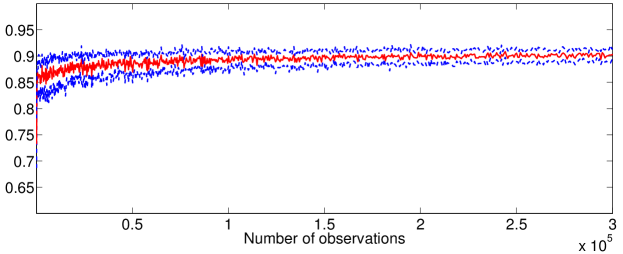
(a) The BOEM algorithm without averaging.

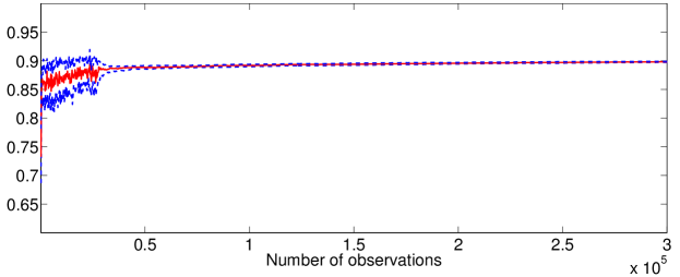
(b) The BOEM algorithm with averaging.

Figure 1: Estimation of $\phi$.

We now discuss the role of $\{\tau_{n}\}_{n\geq 0}$. Figure 2 displays the empirical variance, when estimating $\phi$, computed with $100$ independent Monte Carlo runs, for different numbers of observations and, for both the BOEM algorithm and its averaged version. We consider four polynomial rates $\tau_{n}\sim n^{b}$, $b\in\{1.2,1.8,2,2.5\}$. Figure 2a shows that the choice of $\{\tau_{n}\}_{n\geq 0}$ has a great impact on the empirical variance of the (non averaged) BOEM path $\{\theta_{n}\}_{n\geq 0}$. To reduce this variability, a solution could consist in increasing the block sizes $\tau_{n}$ at a larger. The influence of the block size sequence $\tau_{n}$ is greatly reduced with the averaging procedure as shown in Figure 2b. We will show in Section 5 that averaging really improves the rate of convergence of the BOEM algorithm.

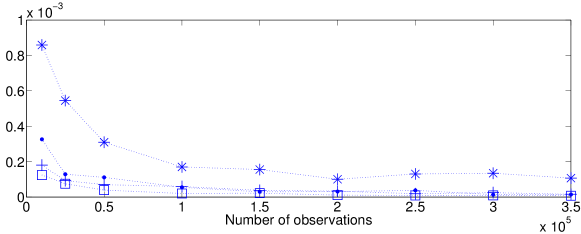
(a) The BOEM algorithm, without averaging

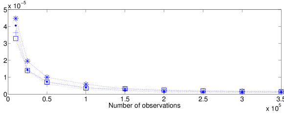
(b) The BOEM algorithm, with averaging

Figure 2: The BOEM algorithm: empirical variance of the estimation of $\phi$ after $n=0.5\ell\,\cdot 10^{5}$ observations ($\ell\in\{1,\cdots,7\}$) for different block size schemes $\tau_{n}\sim n^{1.2}$ (stars), $\tau_{n}\sim n^{1.8}$ (dots), $\tau_{n}\sim n^{2}$ (crosses) and $\tau_{n}\sim n^{2.5}$ (squares).

3.2 Finite state-space HMM

We consider a Gaussian mixture process with Markov dependence of the form: $Y_{t}=X_{t}+V_{t}$ where $\{X_{t}\}_{t\geq 0}$ is a Markov chain taking values in $\mathbb{X}\stackrel{{\scriptstyle\mathrm{def}}}{{=}}\{x_{1},\dots,x_{d}\}$, with initial distribution $\chi$ and a $d\times d$ transition matrix $m$. $\{V_{t}\}_{t\geq 0}$ are i.i.d. $\mathcal{N}(0,v)$ r.v., independent from $\{X_{t}\}_{t\geq 0}$, i.e., for all $(x,y)\in\mathbb{X}\times\mathbb{Y}$,

$$g_{\theta}(x,y)\stackrel{{\scriptstyle\mathrm{def}}}{{=}}(2\pi v)^{-1/2}\exp\left\{-\frac{(y-x)^{2}}{2v}\right\}\;,$$

where $\theta\stackrel{{\scriptstyle\mathrm{def}}}{{=}}\left(v,x_{1:d},(m_{i,j})_{i,j=1}^{d}\right)$. The true transition matrix is given by

$$m=\begin{pmatrix}0.5&0.05&0.1&0.15&0.15&0.05\\ 0.2&0.35&0.1&0.15&0.05&0.15\\ 0.1&0.1&0.6&0.05&0.05&0.1\\ 0.02&0.03&0.1&0.7&0.1&0.05\\ 0.1&0.05&0.13&0.02&0.6&0.1\\ 0.1&0.1&0.13&0.12&0.1&0.45\end{pmatrix}\;.$$

In the experiments below, the initial distribution below is chosen as the uniform distribution on $\mathbb{X}$. The statistics used to estimate $\theta$ are, for all $(i,j)\in\{1,\cdots,d\}$ and all $(x,x^{\prime})\in\mathbb{X}^{2}$,

$$S^{i,0}(x,x^{\prime},y) =\mathbf{1}_{x_{i}}(x^{\prime})\;,\quad\hskip 11.38092ptS^{i,1}(x,x^{\prime},y)=y\mathbf{1}_{x_{i}}(x^{\prime})\;,$$ (9)

$$S^{i,2}(x,x^{\prime},y) =y^{2}\mathbf{1}_{x_{i}}(x^{\prime})\;,\quad S_{i,j}(x,x^{\prime},y)=\mathbf{1}_{x_{i}}(x)\mathbf{1}_{x_{j}}(x^{\prime})\;.$$

The online computation of these intermediate quantities is given [3, Section $2.2$]. The computations below are performed for each statistic in (9). Define, for all $x\in\mathbb{X}$, $\phi_{0}(x)=\chi(x)$ and $\rho_{0}(x)=0$.

1. For $t\in\{1,\cdots,\tau\}$, compute, for any $x\in\mathbb{X}$,

   $$\phi_{t}(x)=\frac{\sum_{x^{\prime}\in\mathbb{X}}\phi_{t-1}(x^{\prime})m_{x^{\prime},x}g_{\theta}(x,Y_{t+T})}{\sum_{x^{\prime},x^{\prime\prime}\in\mathbb{X}}\phi_{t-1}(x^{\prime})m_{x^{\prime},x^{\prime\prime}}g_{\theta}(x^{\prime\prime},Y_{t+T})}\;,$$

   and

   $$r_{t}(x,x^{\prime})=\frac{\phi_{t-1}(x^{\prime})m_{x^{\prime},x}}{\sum_{x^{\prime\prime}\in\mathbb{X}}\phi_{t-1}(x^{\prime\prime})m_{x^{\prime\prime},x}}\;.$$

   $$\rho_{t}(x)=\sum_{x^{\prime}\in\mathbb{X}}\left[\frac{1}{t}S(x,x^{\prime},Y_{t+T})+\left(1-\frac{1}{t}\right)\rho_{t-1}(x^{\prime})\right]r_{t}(x,x^{\prime})\;.$$

2. Set

   $$\bar{S}_{\tau}^{\chi,T}(\theta,\mathbf{Y})=\sum_{x\in\mathbb{X}}\rho_{\tau}(x)\phi_{\tau}(x)\;.$$

At the end of the block, the new estimate is given, for all $(i,j)\in\{1,\cdots,d\}^{2}$ by (the dependence on $\mathbf{Y}$, $\theta$, $\chi$, $T$ and $\tau$ is dropped from the notation)

$$m_{i,j}=\frac{\bar{S}_{i,j}}{\sum_{j=1}^{d}\bar{S}_{i,j}}\;,\;x_{i}=\frac{\bar{S}^{i,1}}{\bar{S}^{i,0}},\;v=\sum_{i=1}^{d}\bar{S}^{i,2}+\sum_{i=1}^{d}x_{i}^{2}\bar{S}^{i,0}-2\sum_{i=1}^{d}x_{i}\bar{S}^{i,1}\;.$$

We first compare the averaged BOEM algorithm to the online EM (OEM) procedure of [3] combined with a Polyak-Ruppert averaging (see [28]). Note that the convergence of the OEM algorithm is still an open problem. In this case, we want to estimate the variance $v$ and the states $\{x_{1},\dots,x_{d}\}$. All the runs are started from $v=2$ and from the initial states $\{-1;0;.5;2;3;4\}$. The algorithm in [3] follows a stochastic approximation update and depends on a step-size sequence $\{\gamma_{n}\}_{n\geq 0}$. It is expected that the rate of convergence in $\mathrm{L}_{2}$ after $n$ observations is $\gamma_{n}^{1/2}$ (and $n^{-1/2}$ for its averaged version) - this assertion relies on classical results for stochastic approximation. We prove in Section 5 that the rate of convergence of the BOEM algorithm is $n^{-b/(2(b+1))}$ (and $n^{-1/2}$ for its averaged version) when $\tau_{n}\propto n^{b}$. Therefore, we set $\tau_{n}=n^{1.1}$ and $\gamma_{n}=n^{-0.53}$. Figure 3 displays the empirical median and first and last quartiles for the estimation of $v$ with both algorithms and their averaged versions as a function of the number of observations. These estimates are obtained over $100$ independent Monte Carlo runs. Both the BOEM and the OEM algorithms converge to the true value of $v$ and the averaged versions reduce the variability of the estimation. Figure 4 shows the similar behavior of both averaged algorithms for the estimation of $x_{1}$ in the same experiment. Some supplementary graphs on the estimation of the states can be found in [20, Section $4$]).

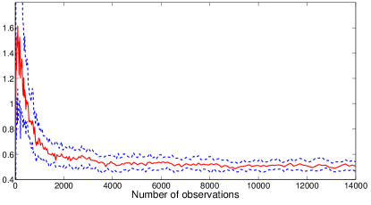
(a) The BOEM algorithm.

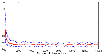
(b) The OEM algorithm.

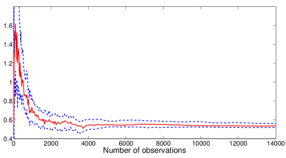
(c) The averaged BOEM algorithm.

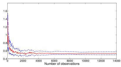
(d) The averaged OEM algorithm.

Figure 3: Estimation of $v$ using the online EM and the BOEM algorithms (top) and their averaged versions (bottom). Each plot displays the empirical median (bold line) and the first and last quartiles (dotted lines) over $100$ independent Monte Carlo runs with $\tau_{n}=n^{1.1}$ and $\gamma_{n}=n^{-0.53}$.

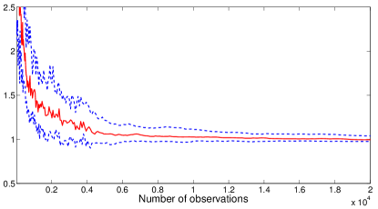
(a) The averaged BOEM algorithm.

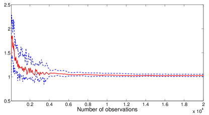
(b) The averaged OEM algorithm.

Figure 4: Estimation of $x_{1}$ using the averaged OEM and the averaged BOEM algorithms. Each plot displays the empirical median (bold line) and the first and last quartiles (dotted lines) over $100$ independent Monte Carlo runs with $\tau_{n}=n^{1.1}$ and $\gamma_{n}=n^{-0.53}$. The first ten observations are omitted for a better visibility.

We now compare the averaged BOEM algorithm to a recursive maximum likelihood (RML) procedure (see [23, 30]) combined with Polyak-Ruppert averaging (see [28]). We want to estimate the variance $v$ and the transition matrix $m$. All the runs are started from $v=2$ and from a matrix $m$ with each entry equal to $1/d$. The RML algorithm follows a stochastic approximation update and depends on a step-size sequence $\{\gamma_{n}\}_{n\geq 0}$ which is chosen in the same way as above. Therefore, for a fair comparison, the RML algorithm (resp. the BOEM algorithm) is run with $\gamma_{n}=n^{-0.53}$ (resp. $\tau_{n}=n^{1.1}$). Figure 5 displays the empirical median and empirical first and last quartiles of the estimation of $m(1,1)$ as a function of the number of observations over $100$ independent Monte Carlo runs. For both algorithms, the bias and the variance of the estimation decrease as $n$ increases. Nevertheless, the bias and/or the variance of the averaged BOEM algorithm decrease faster than those of the averaged RML algorithm (similar graphs have been obtained for the estimation of the other entries of the matrix $m$ and for the estimation of $v$; see [20, Section $4$]). As a conclusion, it is advocated to use the averaged BOEM algorithm instead of the averaged RML algorithm.

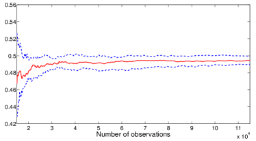
(a) The averaged BOEM algorithm.

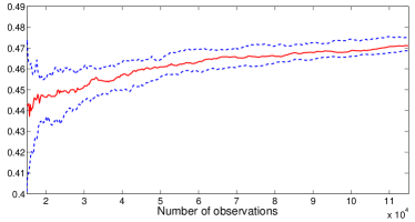
(b) The averaged RML algorithm.

Figure 5: Empirical median (bold line) and first and last quartiles (dotted line) for the estimation of $m(1,1)$ using the averaged RML algorithm (right) and the averaged BOEM algorithm (left). The true values is $m(1,1)=0.5$ and the averaging procedure is starter after $10000$ observations. The first $10000$ observations are not displayed for a better clarity.

4 Convergence of the Block Online EM algorithms

4.1 Assumptions

Consider the following assumptions.

• 1. There exist continuous functions $\phi:\Theta\to\mathbb{R}$, $\psi:\Theta\to\mathbb{R}^{d}$ and $S:\mathbb{X}\times\mathbb{X}\times\mathbb{Y}\to\mathbb{R}^{d}$ s.t.

     $$\log m_{\theta}(x,x^{\prime})+\log g_{\theta}(x^{\prime},y)=\phi(\theta)+\left\langle S(x,x,^{\prime},y),\psi(\theta)\right\rangle\;,$$

     where $\left\langle\cdot,\cdot\right\rangle$ denotes the scalar product on $\mathbb{R}^{d}$.

  2. There exists an open subset $\mathcal{S}$ of $\mathbb{R}^{d}$ that contains the convex hull of $S(\mathbb{X}\times\mathbb{X}\times\mathbb{Y})$.

  3. There exists a continuous function $\bar{\theta}:\mathcal{S}\to\Theta$ s.t. for any $s\in\mathcal{S}$,

     $$\bar{\theta}(s)=\mathrm{argmax}_{\theta\in\Theta}\;\left\{\phi(\theta)+\left\langle s,\psi(\theta)\right\rangle\right\}\;.$$

• There exist $\sigma_{-}$ and $\sigma_{+}$ s.t. for any $\left(x,x^{\prime}\right)\in\mathbb{X}^{2}$ and any $\theta\in\Theta$, $0<\sigma_{-}\leq m_{\theta}(x,x^{\prime})\leq\sigma_{+}$. Set $\rho\stackrel{{\scriptstyle\mathrm{def}}}{{=}}1-(\sigma_{-}/\sigma_{+})\;.$

AA2, often referred to as the strong mixing condition, is commonly used to prove the forgetting property of the initial condition of the filter, see e.g. [10, 11]. This assumption holds for example if $\mathbb{X}$ is finite or for linear state-spaces with truncated gaussian state and measurement noises. More generally, this condition holds when $\mathbb{X}$ is compact. Note in addition that by [25, Theorem $16.0.2$], AA2 implies that the Markov kernel $M_{\theta}$ has a unique invariant distribution which guarantees the existence of the unique invariant distribution $\pi_{\theta}$ for $K_{\theta}$.

We now introduce assumptions on the observation process $\mathbf{Y}\stackrel{{\scriptstyle\mathrm{def}}}{{=}}\{Y_{k}\}_{k\in\mathbb{Z}}$. It is defined on some probability space $(\Omega,\mathcal{F},\mathbb{P})$. We stress that this process is not necessarily the observation of an HMM. Let

$$\mathcal{F}_{k}^{\mathbf{Y}}\stackrel{{\scriptstyle\mathrm{def}}}{{=}}\sigma\left(\{Y_{u}\}_{u\leq k}\right)\quad\mbox{and}\quad\mathcal{G}_{k}^{\mathbf{Y}}\stackrel{{\scriptstyle\mathrm{def}}}{{=}}\sigma\left(\{Y_{u}\}_{u\geq k}\right)$$ (10)

be $\sigma$-fields associated to $\mathbf{Y}$. We also define the $\beta$-mixing coefficients by, see [8],

$$\beta^{\mathbf{Y}}(n)=\underset{u\in\mathbb{Z}}{\sup}\,\underset{B\in\mathcal{G}_{u+n}^{\mathbf{Y}}}{\sup}\,\mathbb{E}\left[|\mathbb{P}(B|\mathcal{F}_{u}^{\mathbf{Y}})-\mathbb{P}(B)|\right]\;,\forall\;n\geq 0\;.$$ (11)

• -($p$) $\mathbb{E}\left[\sup_{x,x^{\prime}\in\mathbb{X}^{2}}\,|S(x,x^{\prime},Y_{0})|^{p}\right]<+\infty$.

• 1. $\mathbf{Y}$ is a $\beta$-mixing stationary sequence such that there exist $C\in[0,1)$ and $\beta\in(0,1)$ satisfying, for any $n\geq 0$, $\beta^{\mathbf{Y}}(n)\leq C\beta^{n}$, where $\beta^{\mathbf{Y}}$ is defined in (11).

  2. $\mathbb{E}\left[|\log b_{-}(Y_{0})|+|\log b_{+}(Y_{0})|\right]<+\infty$ where

     $$b_{-}(y) \stackrel{{\scriptstyle\mathrm{def}}}{{=}}\inf_{\theta\in\Theta}\int g_{\theta}(x,y)\lambda(\mathrm{d}x)\;,$$

     $$b_{+}(y) \stackrel{{\scriptstyle\mathrm{def}}}{{=}}\sup_{\theta\in\Theta}\int g_{\theta}(x,y)\lambda(\mathrm{d}x)\;.$$

Upon noting that, for all $n\geq 0$, $\beta^{\mathbf{Y}}(n)\leq\beta^{(\mathbf{X},\mathbf{Y})}(n)$, we can prove that AA4(a) holds when $\mathbf{Y}$ is the observation process of a an HMM under classical geometric ergodicity conditions [25, Chapter $15$] and [5, Chapter $14$].

• There exists $c>0$ and $a>1$ such that for all $n\geq 1$, $\tau_{n}=\lfloor cn^{a}\rfloor$.

For $p>0$ and $Z$ a random variable measurable w.r.t. the $\sigma$-algebra $\sigma\left(Y_{n},n\in\mathbb{Z}\right)$, set $\left\|Z\right\|_{p}\stackrel{{\scriptstyle\mathrm{def}}}{{=}}\left(\mathbb{E}\left[|Z|^{p}\right]\right)^{1/p}$.

• -($p$) There exists $b\geq(a+1)/2a$ (where $a$ is defined in AA5) such that, for any $n\geq 0$,

  $$\left\|S_{n}-\widetilde{S}_{n}\right\|_{p}=O(\tau_{n+1}^{-b})\;,$$

  where $\widetilde{S}_{n}$ is the Monte Carlo approximation of $S_{n}$ which is defined by (6).

AA6 gives a $\mathrm{L}_{p}$ control of the Monte Carlo error on each block. In [15, Theorem $1$], such bounds are given for Sequential Monte Carlo algorithms. Practical conditions to ensure AA6 are given in [21] in the case of Sequential Monte Carlo methods.

4.2 The limiting EM algorithm

In the sequel, $\mathcal{M}(\mathbb{X})$ denotes the set of all probability distributions on $(\mathbb{X},\mathcal{X})$.

Theorem 4.1.

Let $\bar{p}>2$. Assume that AA1-A2, AA3-($\bar{p}$) and AA4 hold.

1. For any $\theta\in\Theta$, there exists a r.v. $\mathsf{S}(\theta,\mathbf{Y})$ s.t.

   $$\underset{\theta\in\Theta,\,\chi\in\mathcal{M}(\mathbb{X})}{\sup}\left|\mathbb{E}^{\chi,-\tau-1}_{\theta}\left[S(X_{-1},X_{0},Y_{0})\middle|Y_{-\tau:\tau}\right]-\mathsf{S}(\theta,\mathbf{Y})\right|\\ \leq C\rho^{\tau}\underset{(x,x^{\prime})\in\mathbb{X}^{2}}{\sup}\left|S(x,x^{\prime},Y_{0})\right|\;,\quad\mathbb{P}\mathrm{-a.s.}\;,$$ (12)

   where $C$ is a finite constant. Define for all $\theta\in\Theta$,

   $$\bar{\mathrm{S}}(\theta)\stackrel{{\scriptstyle\mathrm{def}}}{{=}}\mathbb{E}\left[\mathsf{S}(\theta,\mathbf{Y})\right]\;.$$ (13)

2. $\theta\mapsto\bar{\mathrm{S}}(\theta)$ is continuous on $\Theta$ and for any $T>0$,

   $$\bar{S}_{\tau}^{\chi,T}(\theta,\mathbf{Y})\underset{\tau\rightarrow+\infty}{\longrightarrow}\bar{\mathrm{S}}(\theta)\;,\quad\mathbb{P}\mathrm{-a.s.}\;,$$ (14)

   where $\bar{S}_{\tau}^{\chi,T}(\theta,\mathbf{Y})$ is defined by (4).

3. Assume in addition that AA6-($\bar{p}$) holds. For any $p\in(2,\bar{p})$, there exists a constant $C$ s.t. for any $n\geq 1$,

   $$\left\|\widetilde{S}_{n}-\bar{\mathrm{S}}(\theta_{n})\right\|_{p}\leq\frac{C}{\sqrt{\tau_{n+1}}}\;,$$

   where $\widetilde{S}_{n}$ is the Monte Carlo approximation of $S_{n}$ defined by (6).

Theorem 4.1 allows to introduce the limiting EM algorithm, defined as the deterministic iterative algorithm $\check{\theta}_{n}=\mathrm{R}(\check{\theta}_{n-1})$ where

$$\mathrm{R}(\theta)\stackrel{{\scriptstyle\mathrm{def}}}{{=}}\bar{\theta}\left(\bar{\mathrm{S}}(\theta)\right)\;.$$ (15)

The limiting EM can be seen as an EM algorithm applied as if the whole trajectory $\mathbf{Y}$ was observed instead of $Y_{0:T}$. For this limiting EM, the so-called sufficient statistics depend on the observations only through the mean $\mathbb{E}\left[\mathsf{S}(\theta,\mathbf{Y})\right]$. The stationary points of the limiting EM are defined as

$$\mathcal{L}\stackrel{{\scriptstyle\mathrm{def}}}{{=}}\left\{\theta\in\Theta;\;\mathrm{R}(\theta)=\theta\right\}\;.$$ (16)

We show that there exists a Lyapunov function $\mathrm{W}$ w.r.t. to the map $\mathrm{R}$ and the set $\mathcal{L}$ i.e., a continuous function $W$ satisfying the two conditions:

1. for all $\theta\in\Theta$, $\mathrm{W}\circ\mathrm{R}(\theta)-\mathrm{W}(\theta)\geq 0\;,$

2. for all compact set $\mathcal{K}\subset\Theta\setminus\mathcal{L}$, $\inf_{\theta\in\mathcal{K}}\left\{\mathrm{W}\circ\mathrm{R}(\theta)-\mathrm{W}(\theta)\right\}>0\;.$

For such a function, the sequence $\{\mathrm{W}(\check{\theta}_{k})\}_{k\geq 0}$ is nondecreasing and $\{\check{\theta}_{k}\}_{k\geq 0}$ converges to $\mathcal{L}$.

Define, for any $m\geq 0$, $\theta\in\Theta$ and probability distribution $\chi$ on $(\mathbb{X},\mathcal{X})$,

$$p_{\theta}^{\chi}\left(Y_{1}\middle|Y_{-m:0}\right)\\ \stackrel{{\scriptstyle\mathrm{def}}}{{=}}\frac{\int\chi(\mathrm{d}x_{-m})g_{\theta}(x_{-m},Y_{m})\prod_{i=-m+1}^{1}\left\{m_{\theta}(x_{i-1},x_{i})g_{\theta}(x_{i},Y_{i})\right\}\lambda(\mathrm{d}x_{-m+1:1})}{\int\chi(\mathrm{d}x_{-m})g_{\theta}(x_{-m},Y_{m})\prod_{i=-m+1}^{0}\left\{m_{\theta}(x_{i-1},x_{i})g_{\theta}(x_{i},Y_{i})\right\}\lambda(\mathrm{d}x_{-m+1:0})}\;.$$

By [13, Lemma $2$ and Proposition $1$], under AA1-A4, for any $\theta\in\Theta$, there exists a random variable $\log p_{\theta}\left(Y_{1}\middle|Y_{-\infty:0}\right)$, such that for any probability distribution $\chi$ on $(\mathbb{X},\mathcal{X})$, $\log p_{\theta}\left(Y_{1}\middle|Y_{-\infty:0}\right)$ is the a.s. limit of $\log p_{\theta}^{\chi}\left(Y_{1}\middle|Y_{-m:0}\right)$ as $m\to+\infty$ and

$$T^{-1}\ell_{\theta,T}^{\chi}(\mathbf{Y})\underset{T\to+\infty}{\longrightarrow}\ell(\theta)\stackrel{{\scriptstyle\mathrm{def}}}{{=}}\mathbb{E}\left[\log p_{\theta}\left(Y_{1}\middle|Y_{-\infty:0}\right)\right]\;,\;\mathbb{P}\mathrm{-a.s.}\;,$$ (17)

where $\ell_{\theta,T}^{\chi}(\mathbf{Y})$ is the log-likelihood defined by (3). The function $\theta\mapsto\ell(\theta)$ may be interpreted as the limiting log-likelihood. We consider the function $W$, given, for all $\theta\in\Theta$, by

$$\mathrm{W}(\theta)\stackrel{{\scriptstyle\mathrm{def}}}{{=}}\exp\left\{\ell(\theta)\right\}\;.$$ (18)

To identify the stationary points of the limiting EM algorithm as the stationary points of $\ell$, we introduce an additional assumption.

• 1. For any $y\in\mathbb{Y}$ and for all $(x,x^{\prime})\in\mathbb{X}^{2}$, $\theta\mapsto g_{\theta}(x,y)$ and $\theta\mapsto m_{\theta}(x,x^{\prime})$ are continuously differentiable on $\Theta$.

  2. $\mathbb{E}\left[\phi(\mathbf{Y}_{0})\right]<+\infty$ where

     $$\phi(y)\stackrel{{\scriptstyle\mathrm{def}}}{{=}}\underset{\theta\in\Theta}{\sup}\;\underset{(x,x^{\prime})\in\mathbb{X}^{2}}{\sup}\left|\nabla_{\theta}\log m_{\theta}(x,x^{\prime})+\nabla_{\theta}\log g_{\theta}(x^{\prime},y)\right|\;.$$

Proposition 4.2.

Assume that AA1-A2, AA3-$(1)$ and AA4 hold. Then, the function $\mathrm{W}$ given by (18) is a Lyapunov function for $(\mathrm{R},\mathcal{L})$. Assume in addition that AA7 holds. Then, $\theta\mapsto\ell(\theta)$ is continuously differentiable and

$$\mathcal{L}=\left\{\theta\in\Theta;\;\mathrm{R}(\theta)=\theta\right\}=\{\theta\in\Theta;\;\nabla\ell(\theta)=0\}\;.$$

Proposition 4.2 is proved in Section 6.2.

Remark 4.3.

In the case where $\{Y_{k}\}_{k\geq 0}$ is the observation process of the stationary HMM $\{(X_{k},Y_{k})\}_{k\geq 0}$ parameterized by $\theta_{\star}\in\Theta$, we can build a two-sided stationary extension of this process to obtain a sequence of observations $\{Y_{k}\}_{k\in\mathbb{Z}}$. Following [13, Proposition $3$], the quantity $\ell(\theta)$ can be written as

$$\ell(\theta) =\mathbb{E}_{\theta_{\star}}\left[\lim_{m\to+\infty}\log p_{\theta}(Y_{1}|Y_{-m:0})\right]$$

$$=\lim_{m\to+\infty}\mathbb{E}_{\theta_{\star}}\left[\log p_{\theta}(Y_{1}|Y_{-m:0})\right]$$

$$=\lim_{m\to+\infty}\mathbb{E}_{\theta_{\star}}\left[\mathbb{E}_{\theta_{\star}}\left[\log p_{\theta}(Y_{1}|Y_{-m:0})\middle|Y_{-m:0}\right]\right]\;,$$

where $p_{\theta}(Y_{1}|Y_{-m:0})$ is the conditional distribution under the stationary distribution. Since

$$\mathbb{E}_{\theta_{\star}}\left[\log p_{\theta_{\star}}(Y_{1}|Y_{-m:0})\middle|Y_{-m:0}\right]-\mathbb{E}_{\theta_{\star}}\left[\log p_{\theta}(Y_{1}|Y_{-m:0})\middle|Y_{-m:0}\right]$$

is the Kullback-Leibler divergence between $p_{\theta_{\star}}(Y_{1}|Y_{-m:0})$ and $p_{\theta}(Y_{1}|Y_{-m:0})$, for any $\theta\in\Theta$, $\ell(\theta_{\star})-\ell(\theta)\geq 0$ and $\theta_{\star}$ is a maximizer of $\theta\mapsto\ell(\theta)$. If in addition $\theta_{\star}$ lies in the interior of $\Theta$, then $\theta_{\star}\in\mathcal{L}$.

The following proposition gives sufficient conditions for the convergence of the limiting EM algorithm and the Monte Carlo BOEM algorithm to the set $\mathcal{L}$.

Theorem 4.4.

Let $\bar{p}>2$. Assume that AA1-A2, AA3-($\bar{p}$) and AA4 hold. Assume in addition that $\mathrm{W}(\mathcal{L})$ has an empty interior. For any initial value $\check{\theta}_{0}\in\Theta$ , there exists $w_{\star}$ s.t. $\{\check{\theta}_{k}\}_{k\geq 0}$ converges to $\{\theta\in\mathcal{L};\;\mathrm{W}(\theta)=w_{\star}\}$. If in addition AA5 and AA6-($\bar{p}$) hold, then the sequence $\{\theta_{n}\}_{n\geq 0}$ converges $\mathbb{P}\mathrm{-a.s.}$ to the same stationary points.

Theorem 4.4 is a direct application of Proposition A.1 for the limiting EM algorithm. The proof for the Monte Carlo BOEM algorithm is detailed in Section 6.3. By Sard’s theorem if $\mathrm{W}$ is at least $d_{\theta}$ (where $\Theta\subset\mathbb{R}^{d_{\theta}}$) continuously differentiable, then $\mathrm{W}(\mathcal{L})$ has Lebesgue measure $0$ and hence has an empty interior.

5 Rate of convergence of the Block Online EM algorithms

We address the rate of convergence of the Monte Carlo BOEM algorithms to a point $\theta_{\star}\in\mathcal{L}$. It is assumed that

• 1. $\bar{\mathrm{S}}$ and $\bar{\theta}$ are twice continuously differentiable on $\Theta$ and $\mathcal{S}$.

  2. There exists $0<\gamma<1$ s.t. the spectral radius of $\nabla_{s}(\bar{\mathrm{S}}\circ\bar{\theta})_{s=\bar{\mathrm{S}}(\theta_{\star})}$ is lower than $\gamma$.

Hereafter, for any sequence of random variables $\{Z_{n}\}_{n\geq 0}$, write $Z_{n}=O_{\mathrm{L}_{p}}(1)$ if $\sup_{n}\mathbb{E}\left[|Z_{n}|^{p}\right]<\infty$ and $Z_{n}=O_{\mathrm{a.s}}(1)$ if $\sup_{n}|Z_{n}|<+\infty$ $\mathbb{P}\mathrm{-a.s.}$

Theorem 5.1.

Let $\bar{p}>2$. Assume that AA2, AA3-($\bar{p}$), AA4-A5, AA6-($\bar{p}$) and AA8 hold. Then, for any $p\in(2,\bar{p})$,

$$\sqrt{\tau_{n}}\ \left[\theta_{n}-\theta_{\star}\right]\mathbf{1}_{\lim_{n}\theta_{n}=\theta_{\star}}=O_{\mathrm{L}_{p}}(1)+\frac{1}{\sqrt{\tau_{n}}}O_{\mathrm{L}_{p/2}}(1)O_{\mathrm{a.s}}\left(1\right)\;.$$ (19)

In (19), the rate is a function of the number of updates (i.e. the number of iterations of the algorithm). Theorem 5.2 shows that the averaging procedure reduces the influence of the block-size schedule: the rate of convergence is proportional to $T_{n}^{1/2}$ i.e. to the inverse of the square root of the total number of observations up to iteration $n$.

Theorem 5.2.

Let $\bar{p}>2$. Assume that AA2, AA3-($\bar{p}$), AA4-A5, AA6-($\bar{p}$) and AA8 hold. Then, for any $p\in(2,\bar{p})$,

$$\sqrt{T_{n}}\left[\widetilde{\theta}_{n}-\theta_{\star}\right]\mathbf{1}_{\lim_{n}\theta_{n}=\theta_{\star}}=O_{\mathrm{L}_{p}}(1)+\frac{n}{\sqrt{T_{n}}}O_{\mathrm{L}_{p/2}}(1)O_{\mathrm{a.s}}\left(1\right)\;.$$ (20)

Theorems 5.1 and 5.2 give the rates of convergence as a function of the number of updates but they can also be studied as a function of the number of observations. Let $\{\theta^{\text{int}}_{k}\}_{k\geq 0}$ (resp. $\{\widetilde{\theta}^{\text{int}}_{k}\}_{k\geq 0}$) be such that, for any $k\geq 0$, $\theta^{\text{int}}_{k}$ (resp. $\widetilde{\theta}^{\text{int}}_{k}$) is the value $\theta_{n}$ (resp. $\widetilde{\theta}_{n}$), where $n$ is the only integer such that $k\in[T_{n}+1,T_{n+1}]$. The sequences $\{\theta^{\text{int}}_{k}\}_{k\geq 0}$ and $\{\widetilde{\theta}^{\text{int}}_{k}\}_{k\geq 0}$ are piecewise constant and their values are updated at times $\{T_{n}\}_{n\geq 1}$.

By Theorem 5.1, the rate of convergence of $\{\theta^{\text{int}}_{k}\}_{k\geq 0}$ is given (up to a multiplicative constant) by $k^{-a/(2(a+1))}$, where $a$ is given by AA5. This rates is slower than $k^{-1/2}$ and depends on the block-size sequence (through $a$). On the contrary, by Theorem 5.2, the rate of convergence of $\{\widetilde{\theta}^{\text{int}}_{k}\}_{k\geq 0}$ is given (up to a multiplicative constant) by $k^{-1/2}$, for any value of $a$. Therefore, this rate of convergence does not depend on the block-size sequence.

6 Proofs

Define, for any initial density $\chi$ on $(\mathbb{X},\mathcal{X})$, any $\theta\in\Theta$, any $\mathbf{y}\in\mathbb{Y}^{\mathbb{Z}}$ and any $r<s\leq t$,

$$\Phi_{\theta,s,t}^{\chi,r}(h,\mathbf{y})\\ \stackrel{{\scriptstyle\mathrm{def}}}{{=}}\frac{\int\chi(x_{r})\{\prod_{i=r}^{t-1}m_{\theta}(x_{i},x_{i+1})g_{\theta}(x_{i+1},y_{i+1})\}\,h(x_{s-1},x_{s},y_{s})\,\lambda(\mathrm{d}x_{r:t})}{\int\chi(x_{r})\{\prod_{i=r}^{t-1}m_{\theta}(x_{i},x_{i+1})g_{\theta}(x_{i+1},y_{i+1})\}\,\lambda(\mathrm{d}x_{r:t})}\;,$$ (21)

for any bounded function $h$ on $\mathbb{X}^{2}\times\mathbb{Y}$. Then, the intermediate quantity of the Block online EM algorithm is (see (4)),

$$\bar{S}_{\tau}^{\chi,T}(\theta,\mathbf{Y})\stackrel{{\scriptstyle\mathrm{def}}}{{=}}\frac{1}{\tau}\sum_{t=T+1}^{T+\tau}\Phi_{\theta,t,T+\tau}^{\chi,T}(S,\mathbf{Y})\;.$$ (22)

Lemma 6.1.

Assume AA1-A2. Let $\mathbf{y}\in\mathbb{Y}^{\mathbb{Z}}$ s.t. $\sup_{x,x^{\prime}}|S(x,x^{\prime},y_{i})|<+\infty$ for any $i\in\mathbb{Z}$. Then for any $r>0$ and any distribution $\chi$ on $(\mathbb{X},\mathcal{X})$, $\theta\mapsto\Phi_{\theta,0,r}^{\chi,-r}(S,\mathbf{y})$ is continuous on $\Theta$.

Proof.

Set $K_{\theta}(x,x^{\prime},y)\stackrel{{\scriptstyle\mathrm{def}}}{{=}}m_{\theta}(x,x^{\prime})g_{\theta}(x^{\prime},y)$. Let $r>0$ and $\chi$ be a distribution on $(\mathbb{X},\mathcal{X})$. By definition of $\Phi_{\theta,0,r}^{\chi,-r}(S,\mathbf{y})$ (see (21)) we have to prove that

$$\theta\mapsto\int\chi(\mathrm{d}x_{-r})\left(\prod_{i=-r}^{r-1}K_{\theta}(x_{i},x_{i+1},y_{i+1})\right)h(x_{-1},x_{0},y_{0})\ \mathrm{d}\lambda(x_{-r+1:r})$$

is continuous for $h(x,x^{\prime},y)=1$ and $h(x,x^{\prime},y)=S(x,x^{\prime},y)$. By AA1(a), the function $\theta\mapsto\prod_{i=-r}^{r-1}K_{\theta}(x_{i},x_{i+1},y_{i+1})\,h(x_{-1},x_{0},y_{0})$ is continuous. In addition, under AA1, for any $\theta\in\Theta$,

$$\left|\prod_{i=-r}^{r-1}K_{\theta}(x_{i},x_{i+1},y_{i+1})\,h(x_{-1},x_{0},y_{0})\right|\\ =|h(x_{-1},x_{0},y_{0})|\exp\left(2r\phi(\theta)+\left\langle\psi(\theta),\sum_{i=-r}^{r-1}S(x_{i},x_{i+1},y_{i+1})\right\rangle\right)\;.$$

Since $\Theta$ is compact, by AA1, there exist constants $C_{1}$ and $C_{2}$ s.t. the supremum in $\theta\in\Theta$ of this expression is bounded above by

$$C_{1}\sup_{x,x^{\prime}}|h(x,x^{\prime},y_{0})|\exp\left(C_{2}\sum_{i=-r}^{r-1}\sup_{x,x^{\prime}}|S(x,x^{\prime},y_{i+1})|\right)\;.$$

Since $\chi$ is a distribution and $\lambda$ is a finite measure, the continuity follows from the dominated convergence theorem. ∎

Let us introduce the following shorthand $S_{s}(x,x^{\prime})\stackrel{{\scriptstyle\mathrm{def}}}{{=}}S(x,x^{\prime},Y_{s})$. Define the shift operator $\vartheta$ onto $\mathbb{Y}^{\mathbb{Z}}$ by $(\vartheta\mathbf{y})_{k}=\mathbf{y}_{k+1}$ for any $k\in\mathbb{Z}$; and by induction, define the $s$-iterated shift operator $\vartheta^{s+1}\mathbf{y}=\vartheta(\vartheta^{s}\mathbf{y})$, with the convention that $\vartheta^{0}$ is the identity operator. For a function $h$, define $\mathrm{osc}(h)\stackrel{{\scriptstyle\mathrm{def}}}{{=}}\sup_{z,z^{\prime}}|h(z)-h(z^{\prime})|$.

6.1 Proof of Theorem 4.1

The proof of Theorem 4.1 relies on auxiliary results about the forgetting properties of HMM. Most of them are really close to published results and their proof is provided in the supplementary material [20, Section $3$]. The main novelty is the forgetting property of the bivariate smoothing distribution.

Proof of i) Note that under AA3-(1), $\mathbb{E}\left[\mathrm{osc}(S_{0})\right]<+\infty$. Under AA2, Proposition A.2(ii) implies that for any $\theta\in\Theta$, there exists a r.v. $\mathsf{S}(\theta,\mathbf{Y})$ s.t. for any $r<s\leq T$,

$$\underset{\theta\in\Theta}{\sup}\;\left|\Phi_{\theta,s,T}^{\chi,r}\left(S,\mathbf{Y}\right)-\mathsf{S}(\theta,\vartheta^{s}\mathbf{Y})\right|\leq\left(\rho^{T-s}+\rho^{s-r-1}\right)\mathrm{osc}(S_{s})\;.$$ (23)

This concludes the proof of (12).

Proof of ii) We introduce the following decomposition: for all $T>0$,

$$\bar{S}_{\tau}^{\chi,T}(\theta,\mathbf{Y})=\frac{1}{\tau}\sum_{t=1}^{\tau}\left[\mathsf{S}(\theta,\vartheta^{t+T}\mathbf{Y})+\left\{\Phi_{\theta,t,\tau}^{\chi,0}\left(S,\vartheta^{T}\mathbf{Y}\right)-\mathsf{S}(\theta,\vartheta^{t+T}\mathbf{Y})\right\}\right]\;,$$

upon noting that by (22), $\bar{S}_{\tau}^{\chi,T}(\theta,\mathbf{Y})=\tau^{-1}\sum_{t=1}^{\tau}\Phi_{\theta,t,\tau}^{\chi,0}\left(S,\vartheta^{T}\mathbf{Y}\right)$. By (21), (23) and AA3-(1) $\mathbb{E}\left[\left|\mathsf{S}(\theta,\mathbf{Y})\right|\right]<+\infty$. Under AA4, the ergodic theorem (see e.g. [1, Theorem 24.1, p.314]) states that, for any fixed $T$,

$$\underset{\tau\to\infty}{\lim}\;\frac{1}{\tau}\sum_{t=1}^{\tau}\mathsf{S}(\theta,\vartheta^{t+T}\mathbf{Y})=\mathbb{E}\left[\mathsf{S}(\theta,\mathbf{Y})\right]\;,\quad\mathbb{P}\mathrm{-a.s.}$$

By (23),

$$\frac{1}{\tau}\sum_{t=1}^{\tau}\left|\Phi_{\theta,t,\tau}^{\chi,0}\left(S,\vartheta^{T}\mathbf{Y}\right)-\mathsf{S}(\theta,\vartheta^{t+T}\mathbf{Y})\right|\leq\frac{1}{\tau}\sum_{t=1}^{\tau}\left(\rho^{\tau-t}+\rho^{t-1}\right)\mathrm{osc}(S_{t+T})\;.$$ (24)

Set $Z_{t}\stackrel{{\scriptstyle\mathrm{def}}}{{=}}\frac{1}{t}\sum_{s=1}^{t}\mathrm{osc}(S_{s+T})$ and $Z_{0}\stackrel{{\scriptstyle\mathrm{def}}}{{=}}0$. Then, by an Abel transform,

$$\frac{1}{\tau}\sum_{t=1}^{\tau}\rho^{t-1}\mathrm{osc}(S_{t+T})=\rho^{\tau-1}Z_{\tau}+\frac{1-\rho}{\tau}\sum_{t=1}^{\tau-1}t\rho^{t-1}Z_{t}\;.$$ (25)

By AA3-(1) and AA4, the ergodic theorem implies that $\lim_{\tau\to\infty}Z_{\tau}=\mathbb{E}\left[\mathrm{osc}(S_{0})\right]$, $\mathbb{P}\mathrm{-a.s.}$ Therefore, $\limsup_{\tau}Z_{\tau}<\infty$, $\mathbb{P}\mathrm{-a.s.}$ Since $\sum_{t\geq 1}t\rho^{t-1}<\infty$, this implies that $\tau^{-1}\sum_{t=1}^{\tau}\rho^{t-1}\mathrm{osc}(S_{t+T})\underset{\tau\to+\infty}{\longrightarrow}0$, $\mathbb{P}\mathrm{-a.s.}$ Similarly,

$$\frac{1}{\tau}\sum_{t=1}^{\tau}\rho^{\tau-t}\mathrm{osc}(S_{t+T})=Z_{\tau}-(1-\rho)\sum_{t=1}^{\tau-1}\rho^{\tau-t-1}Z_{t}+\frac{1-\rho}{\tau}\sum_{t=1}^{\tau-1}t\rho^{t-1}Z_{\tau-t}\;.$$

Using the same arguments as for the second term in (25), we can state that $\lim_{\tau\to\infty}\tau^{-1}\sum_{t=1}^{\tau-1}t\rho^{t-1}Z_{\tau-t}=0$, $\mathbb{P}\mathrm{-a.s.}$ Furthermore,

$$\left|\sum_{t=1}^{\tau-1}\frac{\rho^{\tau-t-1}}{1-\rho}Z_{t}-\mathbb{E}\left[\mathrm{osc}(S_{0})\right]\right|\leq\sum_{t=1}^{\tau-1}\frac{\rho^{\tau-t-1}}{1-\rho}\left|Z_{t}-\mathbb{E}\left[\mathrm{osc}(S_{0})\right]\right|\\ +\;\mathbb{E}\left[\mathrm{osc}(S_{0})\right]\rho^{\tau-1}\;.$$

Since, $\mathbb{P}\mathrm{-a.s.}$, $Z_{\tau}\underset{\tau\to+\infty}{\longrightarrow}\mathbb{E}\left[\mathrm{osc}(S_{0})\right]$, the RHS converges $\mathbb{P}\mathrm{-a.s.}$ to $0$ and

$$\underset{\tau\to+\infty}{\lim}\left|Z_{\tau}-(1-\rho)\sum_{t=1}^{\tau-1}\rho^{\tau-t-1}Z_{t}\right|=0\;,\quad\mathbb{P}\mathrm{-a.s.}$$

Hence, the RHS in (24) converges $\mathbb{P}\mathrm{-a.s.}$ to $0$ and this concludes the proof of (14). We now prove that the function $\theta\mapsto\mathbb{E}\left[\mathsf{S}(\theta,\mathbf{Y})\right]$ is continuous by application of the dominated convergence theorem. By Proposition A.2(ii), for any $\mathbf{y}$ s.t. $\mathrm{osc}(S_{0})<\infty$,

$$\lim_{r\to+\infty}\sup_{\theta\in\Theta}\left|\Phi_{\theta,0,r}^{\chi,-r}(S,\mathbf{y})-\mathsf{S}(\theta,\mathbf{y})\right|=0\;.$$

Then, by Lemma 6.1, $\theta\mapsto\mathsf{S}(\theta,\mathbf{y})$ is continuous for any $\mathbf{y}$ such that $\mathrm{osc}(S_{0})<+\infty$. In addition, $\sup_{\theta\in\Theta}\left|\mathsf{S}(\theta,\mathbf{Y})\right|\leq\sup_{x,x^{\prime}}|S(x,x^{\prime},Y_{0})|$. We then conclude by AA3-(1).

Proof of iii) Let $m_{n},v_{n}$ be positive integers s.t. $1\leq m_{n}\leq\tau_{n+1}$ and $\tau_{n+1}=2v_{n}m_{n}+r_{n}$, where $0\leq r_{n}<2m_{n}$. Set $\Delta p\stackrel{{\scriptstyle\mathrm{def}}}{{=}}p^{-1}-\bar{p}^{-1}$. By the Minkowski inequality combined with Lemmas A.6, A.7 applied with $q_{n}\stackrel{{\scriptstyle\mathrm{def}}}{{=}}2v_{n}m_{n}$, there exists a constant $C$ s.t.

$$\left\|S_{n}-\bar{\mathrm{S}}(\theta_{n})\right\|_{p}\leq C\left[\rho^{m_{n}}+\frac{m_{n}}{\tau_{n+1}}+\beta^{m_{n}\Delta p}+\frac{1}{\sqrt{\tau_{n+1}}}\right]\;.$$

The proof is concluded by choosing $m_{n}=\lfloor-\log\tau_{n+1}/\left(\log\rho\vee\Delta p\log\beta\right)\rfloor$ and by AA6-($\bar{p}$) (since $b$ in AA6-($\bar{p}$) is such that $b\geq 1/2$).

6.2 Proof of Proposition 4.2

 
(Continuity of $\mathrm{R}$ and $\mathrm{W}$) By AA1(c) and Theorem 4.1, the function $\mathrm{R}$ is continuous. Under AA1-A2 and AA4, there exists a continuous function $\ell$ on $\Theta$ s.t. $\lim_{T}T^{-1}\ell_{\theta,T}^{\chi}(\mathbf{Y})=\ell(\theta)$ $\mathbb{P}\mathrm{-a.s.}$ for any distribution $\chi$ on $(\mathbb{X},\mathcal{X})$ and any $\theta\in\Theta$, (see [13, Lemma $2$ and Propositions $1$ and $2$], see also [20, Theorem $3.8$]). Therefore, $\mathrm{W}$ is continuous.

Proof of Proposition 4.2 (i) Under Assumption AA1(a)

$$\frac{1}{T}\log p_{\theta}(x_{0:T},Y_{1:T})=\phi(\theta)+\left\langle\left\{\frac{1}{T}\sum_{t=1}^{T}S(x_{t-1},x_{t},Y_{t})\right\},\psi(\theta)\right\rangle\;,$$

where $p_{\theta}(x_{0:T},Y_{1:T})$ is defined by (1). Upon noting that

$$\int S(x_{t-1},x_{t},Y_{t})\frac{p_{\theta}(x_{0:T},Y_{1:T})}{\int p_{\theta}(z_{0:T},Y_{1:T})\lambda(\mathrm{d}z_{1:T})\chi(\mathrm{d}z_{0})}\lambda(\mathrm{d}x_{1:T})\chi(\mathrm{d}x_{0})\\ =\Phi_{\theta,t,T}^{\chi,0}(S,\mathbf{Y})\;,$$

the Jensen inequality gives, $\mathbb{P}\mathrm{-a.s.}$,

$$\frac{1}{T}\ell_{\mathrm{R}(\theta),T}^{\chi}(\mathbf{Y})-\frac{1}{T}\ell_{\theta,T}^{\chi}(\mathbf{Y})\geq\phi(\mathrm{R}(\theta))+\left\langle\frac{1}{T}\sum_{t=1}^{T}\Phi_{\theta,t,T}^{\chi,0}(S,\mathbf{Y}),\psi(\mathrm{R}(\theta))\right\rangle\\ -\phi(\theta)-\left\langle\frac{1}{T}\sum_{t=1}^{T}\Phi_{\theta,t,T}^{\chi,0}(S,\mathbf{Y}),\psi(\theta)\right\rangle\;.$$ (26)

Under AA1-A4, it holds by Theorem 4.1 and [13, Lemma $2$ and Proposition $1$] (see also [20, Theorem $3.8$]) that for all $\theta\in\Theta$, $\mathbb{P}\mathrm{-a.s.}$,

$$\frac{1}{T}\sum_{t=1}^{T}\Phi_{\theta,t,T}^{\chi,0}(S,\mathbf{Y})\underset{T\to+\infty}{\longrightarrow}\bar{\mathrm{S}}(\theta)\;,\qquad\frac{1}{T}\ell_{\theta,T}^{\chi}(\mathbf{Y})\underset{T\to+\infty}{\longrightarrow}\ln\mathrm{W}(\theta)\;.$$

Therefore, when $T\to+\infty$, (26) implies

$$\ln\left(\mathrm{W}(\mathrm{R}(\theta))/\mathrm{W}(\theta)\right)\geq\phi(\mathrm{R}(\theta))+\left\langle\bar{\mathrm{S}}(\theta),\psi(\mathrm{R}(\theta))\right\rangle-\phi(\theta)-\left\langle\bar{\mathrm{S}}(\theta),\psi(\theta)\right\rangle\;.$$ (27)

By definition of $\bar{\theta}$ and $\mathrm{R}$ (see AA1(c) and (15)), the RHS is non negative. This concludes the proof of Proposition 4.2(i).

Proof of Proposition 4.2 (ii) We prove that $\mathrm{W}\circ\mathrm{R}(\theta)-\mathrm{W}(\theta)=0$ if and only if $\theta\in\mathcal{L}$. Since $\mathrm{W}\circ\mathrm{R}-\mathrm{W}$ is continuous, this implies that $\underset{\theta\in\mathcal{K}}{\inf}\mathrm{W}\circ\mathrm{R}(\theta)-\mathrm{W}(\theta)>0$ for all compact set $\mathcal{K}\subset\Theta\setminus\mathcal{L}$. Let $\theta\in\Theta$ be s.t. $\mathrm{W}\circ\mathrm{R}(\theta)-\mathrm{W}(\theta)=0$. Then, the RHS in (27) is equal to zero. By definition of $\bar{\theta}$, $\mathrm{R}(\theta)=\theta$ and thus $\theta\in\mathcal{L}$. The converse implication is immediate from the definition of $\mathcal{L}$.

Stationary points If in addition AA7 holds, [20, Theorem $3.12$] proves that, for any initial distribution $\chi$ on $(\mathbb{X},\mathcal{X})$,

$$\frac{1}{T}\nabla_{\theta}\ell^{\chi}_{\theta,T}(\mathbf{Y})\underset{T\rightarrow+\infty}{\longrightarrow}\nabla_{\theta}\ell(\theta)\quad\mathbb{P}\mathrm{-a.s.}$$

Therefore,

$$\frac{1}{T}\nabla_{\theta}\ell^{\chi}_{\theta,T}(\mathbf{Y})=\nabla_{\theta}\phi(\theta)+\nabla_{\theta}\psi^{{}^{\prime}}(\theta)\left\{\frac{1}{T}\sum_{t=1}^{T}\Phi_{\theta,t,T}^{\chi,0}(S,\mathbf{Y})\right\}\;,$$

where $A^{\prime}$ is the transpose matrix of $A$. Theorem 4.1 yield, $\mathbb{P}\mathrm{-a.s.}$,

$$\nabla_{\theta}\ell(\theta)=\nabla_{\theta}\phi(\theta)+\nabla_{\theta}\psi^{{}^{\prime}}(\theta)\bar{S}(\theta)\;.$$

The proof follows upon noting that by definition of $\bar{\theta}$, the unique solution to the equation $\nabla_{\theta}\phi(\tau)+\nabla_{\theta}\psi^{{}^{\prime}}(\tau)\bar{S}(\theta)=0$ is $\tau=\mathrm{R}(\theta)$.

6.3 Proof of Theorem 4.4

The proof of Theorem 4.4 relies on Proposition A.1 applied with $T(\theta)\stackrel{{\scriptstyle\mathrm{def}}}{{=}}\mathrm{R}(\theta)$ and with $\theta_{n+1}=\bar{\theta}\left(\widetilde{S}_{\tau_{n+1}}^{\chi_{n},T_{n}}(\theta_{n},\mathbf{Y})\right)$. The key ingredient for this proof is the control of the $\mathrm{L}_{p}$-mean error between the Monte Carlo Block Online EM algorithm and the limiting EM. The proof of this bound is derived in Theorem 4.1 and relies on preliminary lemmas given in Appendix A. The proof of (37) is now close to the proof of [16, Proposition $11$] and is postponed to the supplement paper [20, Section $2.1$].

6.4 Proof of Theorem 5.1

Define $s_{\star}\stackrel{{\scriptstyle\mathrm{def}}}{{=}}\bar{\mathrm{S}}(\theta_{\star})$ and write

$$\bar{\theta}(\widetilde{S}_{n})-\bar{\theta}(s_{\star})=\Upsilon(\widetilde{S}_{n}-s_{\star})+\bar{\theta}(\widetilde{S}_{n})-\bar{\theta}(s_{\star})-\Upsilon(\widetilde{S}_{n}-s_{\star})\;,$$ (28)

where $\Upsilon\stackrel{{\scriptstyle\mathrm{def}}}{{=}}\nabla\bar{\theta}(s_{\star})$. We now derive the rate of convergence of the quantity $\widetilde{S}_{n}-s_{\star}$. Set $\mathrm{G}(s)\stackrel{{\scriptstyle\mathrm{def}}}{{=}}\bar{\mathrm{S}}\circ\bar{\theta}(s)$. Note that under AA8(b), $\rho(\Gamma)\leq\gamma$, where $\Gamma\stackrel{{\scriptstyle\mathrm{def}}}{{=}}\nabla\mathrm{G}(s_{\star})$. Since $\mathrm{G}(s_{\star})=s_{\star}$, we write

$$\widetilde{S}_{n}-s_{\star}=\Gamma\left(\widetilde{S}_{n-1}-s_{\star}\right)+\widetilde{S}_{n}-\mathrm{G}(\widetilde{S}_{n-1})+\mathrm{G}(\widetilde{S}_{n-1})-\mathrm{G}(s_{\star})-\Gamma\left(\widetilde{S}_{n-1}-s_{\star}\right)\;.$$

Define $\{\mu_{n}\}_{n\geq 0}$ and $\{\rho_{n}\}_{n\geq 0}$ s.t. $\mu_{0}=0$, $\rho_{0}=\widetilde{S}_{0}-s_{\star}$ and

$$\mu_{n}\stackrel{{\scriptstyle\mathrm{def}}}{{=}}\Gamma\mu_{n-1}+e_{n}\;,\qquad\rho_{n}\stackrel{{\scriptstyle\mathrm{def}}}{{=}}\widetilde{S}_{n}-s_{\star}-\mu_{n}\;,\qquad n\geq 1\;,$$ (29)

where,

$$e_{n}\stackrel{{\scriptstyle\mathrm{def}}}{{=}}\widetilde{S}_{n}-\bar{\mathrm{S}}(\theta_{n})\;,\qquad n\geq 1\;.$$ (30)

Proposition 6.2.

Assume AA2, AA3-($\bar{p}$), AA4-A5, AA6-($\bar{p}$) and AA8 for some $\bar{p}>2$. Then for any $p\in(2,\bar{p})$,

$$\sqrt{\tau_{n}}\mu_{n}=O_{\mathrm{L}_{p}}(1)\quad\mbox{and}\quad\tau_{n}\rho_{n}\mathbf{1}_{\lim_{n}\theta_{n}=\theta_{\star}}=O_{\mathrm{L}_{p/2}}(1)O_{\mathrm{a.s}}(1)\;.$$

The proof of Proposition 6.2 is on the same lines as the proof of [16, Theorem 6]. The main ingredient is the control of $\left\|\mu_{n}\right\|_{p}$ which is a consequence of [27, Result 178, p. 39] and Theorem 4.1. The detailed proof is thus omitted and postponed to the supplementary material [20, Section $2.2$].

By Proposition 6.2, the first term in (28) gives

$$\sqrt{\tau_{n}}\Upsilon(S_{n}-s_{\star})\mathbf{1}_{\lim_{n}\theta_{n}=\theta_{\star}}=O_{\mathrm{L}_{p}}(1)+\frac{1}{\sqrt{\tau_{n}}}O_{\mathrm{L}_{p/2}}(1)O_{\mathrm{a.s}}\left(1\right)\;.$$

A Taylor expansion with integral remainder term gives the rate of convergence of the second term. This concludes the proof of Theorem 5.1, Eq. (19).

6.5 Proof of Theorem 5.2

In the sequel, for all function $\Xi$ on $\Theta\times\mathbb{Y}^{\mathbb{Z}}$ and all $\upsilon\in\Theta$, we denote by $\mathbb{E}\left[\Xi(\theta,\mathbf{Y})\right]_{\theta=\upsilon}$ the function $\theta\mapsto\mathbb{E}\left[\Xi(\theta,\mathbf{Y})\right]$ evaluated at $\theta=\upsilon$. We preface the proof by the following lemma.

Lemma 6.3.

Assume AA2, AA3-($\bar{p}$), AA4-A5, AA6-($\bar{p}$) and AA8 for some $\bar{p}>2$. For any $p\in(2,\bar{p})$,

$$\underset{n\to+\infty}{\limsup}\;\frac{1}{\sqrt{T_{n+1}}}\;\left\|\sum_{k=1}^{n}\tau_{k+1}e_{k}\right\|_{p}<\infty\;,$$

where $e_{n}$ is given by (30).

Proof.

By AA5 and AA6-($\bar{p}$), we have

$$\underset{n\to+\infty}{\limsup}\;\frac{1}{\sqrt{T_{n+1}}}\;\sum_{k=1}^{n}\tau_{k+1}\left\|\widetilde{S}_{k}-S_{k}\right\|_{p}<\infty\;.$$

Then, it is sufficient to prove that

$$\underset{n\to+\infty}{\limsup}\;\frac{1}{\sqrt{T_{n+1}}}\;\left\|\sum_{k=1}^{n}\tau_{k+1}\left(\bar{S}(\theta_{k})-S_{k}\right)\right\|_{p}<\infty\;.$$

Let $p\in(2,\bar{p})$. In the sequel, $C$ is a constant independent on $n$ and whose value may change upon each appearance. Let $1\leq m_{n}\leq\tau_{n+1}$ and set $v_{n}\stackrel{{\scriptstyle\mathrm{def}}}{{=}}\left\lfloor\frac{\tau_{n+1}}{2m_{n}}\right\rfloor$. By Lemma A.7 applied with $q_{k}\stackrel{{\scriptstyle\mathrm{def}}}{{=}}2v_{k}m_{k}$, we have,

$$\left\|\sum_{k=1}^{n}\tau_{k+1}\left(\bar{S}(\theta_{k})-S_{k}\right)\right\|_{p}\\ \leq C\left(\sum_{k=1}^{n}\{\tau_{k+1}\rho^{m_{k}}+m_{k}\}+\left\|\sum_{k=1}^{n}\{\delta_{k}+\zeta_{k}\}\right\|_{p}\right)\;,$$

where $\delta_{k}$ and $\zeta_{k}$ are defined by

$$\delta_{k} \stackrel{{\scriptstyle\mathrm{def}}}{{=}}\sum_{t=2m_{k}}^{2v_{k}m_{k}}\left\{F_{t,k}(\theta_{k},\mathbf{Y})-\mathbb{E}\left[F_{t,k}(\theta_{k},\mathbf{Y})\middle|\widetilde{\mathcal{F}}_{T_{k}}^{\mathbf{Y}}\right]\right\}\;,$$

$$\zeta_{k} \stackrel{{\scriptstyle\mathrm{def}}}{{=}}\sum_{t=2m_{k}}^{2v_{k}m_{k}}\left\{\mathbb{E}\left[F_{t,k}(\theta_{k},\mathbf{Y})\middle|\widetilde{\mathcal{F}}_{T_{k}}^{\mathbf{Y}}\right]-\mathbb{E}\left[\Phi_{\theta,0,m_{k}}^{\chi,-m_{k}}(S,\mathbf{Y})\right]_{\theta=\theta_{k}}\right\}$$

and where $F_{t,k}(\theta_{k},\mathbf{Y})\stackrel{{\scriptstyle\mathrm{def}}}{{=}}\Phi_{\theta_{k},t,t+m_{k}}^{\chi,t-m_{k}}(S,\vartheta^{T_{k}}\mathbf{Y})$ and $\widetilde{\mathcal{F}}_{T_{k}}^{\mathbf{Y}}$ is given by (41). We will prove below that there exists $C$ s.t.

$$\left\|\zeta_{k}\right\|_{p}\leq C\,\beta^{m_{k}/pb}\tau_{k+1}\;,\qquad\forall k\geq 1$$ (31)

$$\left\|\sum_{k=1}^{n}\delta_{k}\right\|_{p}\leq C\sqrt{T_{n+1}}+C\sum_{k=1}^{n}\tau_{k+1}\beta^{m_{k}/pb}\;,\qquad\forall n\geq 1$$ (32)

so that the proof is concluded by choosing $m_{k}=\lfloor\eta\log\tau_{k+1}\rfloor$, $\eta\stackrel{{\scriptstyle\mathrm{def}}}{{=}}\left(-1/\log\rho\right)\vee\left(-pb/\log\beta\right)$ and by using AA5.

We turn to the proof of (31). By the Berbee Lemma (see [29, Chapter $5$]) and AA4, there exist $C\in[0,1)$ and $\beta\in(0,1)$ s.t. for all $k\geq 1$, there exists a random variable $Y^{\star,(k)}_{T_{k}+m_{k}:T_{k+1}+m_{k}}$ on $(\Omega,\mathcal{F},\mathbb{P})$ independent from $\widetilde{\mathcal{F}}_{T_{k}}^{\mathbf{Y}}$ with the same distribution as $Y_{T_{k}+m_{k}:T_{k+1}+m_{k}}$ and

$$\mathbb{P}\left\{Y^{\star,(k)}_{T_{k}+m_{k}:T_{k+1}+m_{k}}\neq Y_{T_{k}+m_{k}:T_{k+1}+m_{k}}\right\}\leq C\beta^{m_{k}}\;.$$ (33)

Upon noting that $\mathbb{E}\left[F_{t,k}(\theta_{k},\mathbf{Y}^{\star,(k)})\middle|\widetilde{\mathcal{F}}_{T_{k}}^{\mathbf{Y}}\right]=\mathbb{E}\left[F_{t,k}(\theta,\mathbf{Y})\right]_{\theta=\theta_{k}}$, we have

$$\zeta_{k}=\sum_{t=2m_{k}}^{2v_{k}m_{k}}\left\{\mathbb{E}\left[F_{t,k}(\theta_{k},\mathbf{Y})\middle|\widetilde{\mathcal{F}}_{T_{k}}^{\mathbf{Y}}\right]-\mathbb{E}\left[F_{t,k}(\theta_{k},\mathbf{Y}^{\star,(k)})\middle|\widetilde{\mathcal{F}}_{T_{k}}^{\mathbf{Y}}\right]\right\}\;.$$ (34)

Therefore, by setting $\mathcal{A}_{k}\stackrel{{\scriptstyle\mathrm{def}}}{{=}}\{Y^{\star,(k)}_{T_{k}+m_{k}:T_{k+1}+m_{k}}\neq Y_{T_{k}+m_{k}:T_{k+1}+m_{k}}\}$,

$$\left|\zeta_{k}\right| \leq\sum_{t=2m_{k}}^{2v_{k}m_{k}}\mathbb{E}\left[\underset{\theta\in\Theta}{\sup}\left|F_{t,k}(\theta,\mathbf{Y})-F_{t,k}(\theta,\mathbf{Y}^{\star,(k)})\right|\mathbf{1}_{\mathcal{A}_{k}}\middle|\widetilde{\mathcal{F}}_{T_{k}}^{\mathbf{Y}}\right]\;.$$

Minkowski and Holder (with $a\stackrel{{\scriptstyle\mathrm{def}}}{{=}}\bar{p}/p$ and $b^{-1}\stackrel{{\scriptstyle\mathrm{def}}}{{=}}1-a^{-1}$) inequalities, combined with (33), AA4, Lemma A.4 and AA3-($\bar{p}$) yield (31).

We now prove (32). Upon noting that $\delta_{k}$ is $\widetilde{\mathcal{F}}_{T_{k+1}}^{\mathbf{Y}}$-measurable and $\delta_{k}$ is a martingale increment, the Rosenthal inequality (see [17, Theorem 2.12, p.23]) states that $\left\|\sum_{k=1}^{n}\delta_{k}\right\|_{p}\leq C\left(\sum_{k=1}^{n}I_{k}^{(1)}\right)^{1/p}+CI_{n}^{(2)}$ where

$$I_{k}^{(1)}\stackrel{{\scriptstyle\mathrm{def}}}{{=}}\mathbb{E}\left[\left|\delta_{k}\right|^{p}\right]\quad\mbox{and}\quad I_{n}^{(2)}\stackrel{{\scriptstyle\mathrm{def}}}{{=}}\left\|\left(\sum_{k=1}^{n}\mathbb{E}\left[\left|\delta_{k}\right|^{2}\middle|\widetilde{\mathcal{F}}_{T_{k}}^{\mathbf{Y}}\right]\right)^{1/2}\right\|_{p}\;.$$

Using again $\mathbb{E}\left[F_{t,k}(\theta_{k},\mathbf{Y}^{\star,(k)})\middle|\widetilde{\mathcal{F}}_{T_{k}}^{\mathbf{Y}}\right]=\mathbb{E}\left[F_{t,k}(\theta,\mathbf{Y})\right]_{\theta=\theta_{k}}$ and (34)

$$I_{k}^{(1)}\leq C\;\left\|\sum_{t=2m_{k}}^{2v_{k}m_{k}}\left\{F_{t,k}(\theta_{k},\mathbf{Y})-\mathbb{E}\left[F_{t,k}(\theta,\mathbf{Y})\right]_{\theta=\theta_{k}}\right\}\right\|_{p}^{p}+C\;\left\|\zeta_{k}\right\|_{p}^{p}\;.$$

By Lemma A.6 and (31), there exists $C$ s.t. for any $k\geq 1$

$$I_{k}^{(1)}\leq C\left(\tau_{k+1}^{p/2}+\tau_{k+1}^{p}\beta^{m_{k}/b}\right)\;,$$ (35)

and since $2/p<1$, convex inequalities yield $\left(\sum_{k=1}^{n}I_{k}^{(1)}\right)^{1/p}\leq C\sqrt{T_{n+1}}+C\sum_{k=1}^{n}\tau_{k+1}\beta^{m_{k}/pb}$. By the Minkowski and Jensen inequalities, it holds $I_{n}^{(2)}\leq\left(\sum_{k=1}^{n}\{I_{k}^{(1)}\}^{2/p}\right)^{1/2}$. Hence, by (35), $I_{n}^{(2)}\leq C\sqrt{T_{n+1}}+C\sum_{k=1}^{n}\tau_{k+1}\beta^{m_{k}/pb}$. This concludes the proof of (32). ∎

We write $\Sigma_{n}-s_{\star}=\bar{\mu}_{n}+\bar{\rho}_{n}$ with

$$\bar{\mu}_{n}\stackrel{{\scriptstyle\mathrm{def}}}{{=}}\frac{1}{T_{n}}\sum_{k=1}^{n}\tau_{k}\mu_{k-1}\quad\mbox{and}\quad\bar{\rho}_{n}\stackrel{{\scriptstyle\mathrm{def}}}{{=}}\frac{1}{T_{n}}\sum_{k=1}^{n}\tau_{k}\rho_{k-1}\;.$$ (36)

Proposition 6.4.

Assume AA2, AA3-($\bar{p}$), AA4-A5, AA6-($\bar{p}$) and AA8 for some $\bar{p}>2$. For any $p\in(2,\bar{p})$,

$$\sqrt{T_{n}}\bar{\mu}_{n}=O_{\mathrm{L}_{p}}(1)\;,\qquad\frac{T_{n}}{n}\,\bar{\rho}_{n}\mathbf{1}_{\lim_{n}\theta_{n}=\theta_{\star}}=O_{\mathrm{L}_{p/2}}(1)O_{\mathrm{a.s}}(1)\;.$$

Proof.

Set $A\stackrel{{\scriptstyle\mathrm{def}}}{{=}}\left(I-\Gamma\right)$. Under AA8, $A^{-1}$ exists. By (29) and (36),

$$A\sqrt{T_{n}}\bar{\mu}_{n}=-\frac{\tau_{n+1}\mu_{n}}{\sqrt{T_{n}}}+\frac{1}{\sqrt{T_{n}}}\sum_{k=1}^{n}\tau_{k+1}e_{k}+\frac{1}{\sqrt{T_{n}}}\sum_{k=1}^{n}\tau_{k}\left(\frac{\tau_{k+1}}{\tau_{k}}-1\right)\Gamma\mu_{k-1}\;.$$

The result now follows from Proposition 6.2, Lemma 6.3 and AA5. The proof of the second assertion follows from (36) and Proposition 6.2. ∎

Upon noting that $\theta_{\star}=\bar{\theta}(s_{\star})$, we may write, for the averaged sequence,

$$\widetilde{\theta}_{n}-\theta_{\star}=\Upsilon(\Sigma_{n}-s_{\star})+\bar{\theta}(\Sigma_{n})-\bar{\theta}(s_{\star})-\Upsilon(\Sigma_{n}-s_{\star})\;.$$

The first term in this decomposition gives

$$\sqrt{T_{n}}\Upsilon(\Sigma_{n}-s_{\star})\mathbf{1}_{\lim_{n}\theta_{n}=\theta_{\star}}=O_{\mathrm{L}_{p}}(1)+\frac{n}{\sqrt{T_{n}}}O_{\mathrm{L}_{p/2}}(1)O_{\mathrm{a.s}}\left(1\right)\;.$$

By AA8(b), as for the non averaged sequence, a Taylor expansion with integral remainder term gives the result for the second term. This concludes the proof of Theorem 5.2, Eq.(20).

7 Acknowledgments

The authors are grateful to Eric Moulines and Olivier Cappé for their fruitful remarks.

Appendix A Technical results

Proposition A.1 is exactly [16, Proposition $9$] applied with a compact set $\Theta$.

Proposition A.1.

Let $T:\Theta\to\Theta$ and $\mathrm{W}$ be a continuous Lyapunov function relatively to $T$ and to $\mathcal{L}\subset\Theta$. Assume $\mathrm{W}(\mathcal{L})$ has an empty interior and that $\{\theta_{n}\}_{n\geq 0}$ is a sequence lying in $\Theta$ such that

$$\underset{n\to+\infty}{\lim}\left|\mathrm{W}(\theta_{n+1})-\mathrm{W}\circ T(\theta_{n})\right|=0\;.$$ (37)

Then, there exists $w_{\star}$ such that $\{\theta_{n}\}_{n\geq 0}$ converges to $\{\theta\in\mathcal{L};\;\mathrm{W}(\theta)=w_{\star}\}$.

The proof of Proposition A.2 is given in [20, Proposition $3.3$]

Proposition A.2.

Assume AA2. Let $\chi$, $\widetilde{\chi}$ be two distributions on $\left(\mathbb{X},\mathcal{X}\right)$. For any measurable function $h:\mathbb{X}^{2}\times\mathbb{Y}\to\mathbb{R}^{d}$ and any $\mathbf{y}\in\mathbb{Y}^{\mathbb{Z}}$ such that $\sup_{x,x^{\prime}}|h(x,x^{\prime},y_{s})|<+\infty$ for any $s\in\mathbb{Z}$

1. For any $r<s\leq t$ and any $\ell_{1},\ell_{2}\geq 1$,

   $$\underset{\theta\in\Theta}{\sup}\left|\Phi_{\theta,s,t}^{\widetilde{\chi},r}\left(h,\mathbf{y}\right)-\Phi_{\theta,s,t+\ell_{2}}^{\chi,r-\ell_{1}}\left(h,\mathbf{y}\right)\right|\leq\left(\rho^{s-1-r}+\rho^{t-s}\right)\mathrm{osc}(h_{s})\;.$$ (38)

2. For any $\theta\in\Theta$, there exists a function $\mathbf{y}\mapsto\Phi_{\theta}(h,\mathbf{y})$ s.t. for any distribution $\chi$ on $(\mathbb{X},\mathcal{X})$ and any $r<s\leq t$

   $$\underset{\theta\in\Theta}{\sup}\left|\Phi_{\theta,s,t}^{\chi,r}\left(h,\mathbf{y}\right)-\Phi_{\theta}\left(h,\vartheta^{s}\mathbf{y}\right)\right|\leq\left(\rho^{s-1-r}+\rho^{t-s}\right)\mathrm{osc}(h_{s})\;.$$ (39)

Remark A.3.

1. If $\chi=\widetilde{\chi}$, $\ell_{1}=0$ and $\ell_{2}\geq 1$, (38) becomes

   $$\underset{\theta\in\Theta}{\sup}\left|\Phi_{\theta,s,t}^{\chi,r}\left(h,\mathbf{y}\right)-\Phi_{\theta,s,t+\ell_{2}}^{\chi,r}\left(h,\mathbf{y}\right)\right|\leq\rho^{t-s}\mathrm{osc}(h_{s})\;.$$

2. if $\ell_{2}=0$ and $\ell_{1}\geq 1$, (38) becomes

   $$\underset{\theta\in\Theta}{\sup}\left|\Phi_{\theta,s,t}^{\widetilde{\chi},r}\left(h,\mathbf{y}\right)-\Phi_{\theta,s,t}^{\chi,r-\ell_{1}}\left(h,\mathbf{y}\right)\right|\leq\rho^{s-1-r}\mathrm{osc}(h_{s})\;.$$

Lemma A.4 is a consequence of (21) and of Proposition A.2(ii).

Lemma A.4.

Assume AA2. Let $r<s\leq t$ be integers, $\theta\in\Theta$ and $\mathbf{y}\in\mathbb{Y}^{\mathbb{Z}}$, and $h:\mathbb{X}^{2}\times\mathbb{Y}\to\mathbb{R}^{d}$ s.t. for any $s\in\mathbb{Z}$, $\sup_{x,x^{\prime}}|h(x,x^{\prime},y_{s})|<\infty$. Then

$$\left|\Phi_{\theta,s,t}^{\chi,r}\left(h,\mathbf{y}\right)\right|\leq\underset{(x,x^{\prime})\in\mathbb{X}^{2}}{\sup}\left|h(x,x^{\prime},y_{s})\right|\;,\,\left|\Phi_{\theta}\left(h,\vartheta^{s}\mathbf{y}\right)\right|\leq\underset{(x,x^{\prime})\in\mathbb{X}^{2}}{\sup}\left|h(x,x^{\prime},y_{s})\right|\;.$$

For any $L\geq 1$, $m\geq 1$ and any distribution $\chi$ on $(\mathbb{X},\mathcal{X})$, define

$$\kappa_{L,m}^{\chi}(\boldsymbol{\theta},\mathbf{Y})\stackrel{{\scriptstyle\mathrm{def}}}{{=}}\Phi_{\boldsymbol{\theta},L,L+m}^{\chi,L-m}(S,\mathbf{Y})-\mathbb{E}\left[\Phi_{\upsilon,0,m}^{\chi,-m}(S,\mathbf{Y})\right]_{\upsilon=\boldsymbol{\theta}}\;.$$ (40)

We introduce the $\sigma$-algebra $\widetilde{\mathcal{F}}_{T_{n}}$ defined by

$$\widetilde{\mathcal{F}}_{T_{n}}\stackrel{{\scriptstyle\mathrm{def}}}{{=}}\sigma\{\mathcal{F}_{T_{n}}^{\mathbf{Y}},\mathcal{H}_{T_{n}}\}\;,$$ (41)

where $\mathcal{F}_{T_{n}}$ is given by (10) and where $\mathcal{H}_{T_{n}}$ is independent from $\mathbf{Y}$ (the $\sigma$-algebra $\mathcal{H}_{T_{n}}$ is generated by the random variables independent from the observations $\mathbf{Y}$ used to produce the Monte Carlo approximation of $\{S_{k-1}\}_{k=1}^{n}$). Hence, for any positive integer $m$ and any $B\in\mathcal{G}_{T_{n}+m}^{\mathbf{Y}}$, since $\mathcal{H}_{T_{n}}$ is independent from $B$ and from $\mathcal{F}_{T_{n}}^{\mathbf{Y}}$, $\mathbb{P}(B|\widetilde{\mathcal{F}}_{T_{n}})=\mathbb{P}(B|\mathcal{F}_{T_{n}}^{\mathbf{Y}})$. Hence, the mixing coefficients defined in (11) are such that

$$\beta{}(\mathcal{G}_{T_{n}+m}^{\mathbf{Y}},\widetilde{\mathcal{F}}_{T_{n}})=\beta(\mathcal{G}_{T_{n}+m}^{\mathbf{Y}},\mathcal{F}_{T_{n}^{\mathbf{Y}}})\;.$$

Note that $\theta_{n}$ is $\widetilde{\mathcal{F}}_{T_{n}}$- measurable and that $\widetilde{S}_{n}$ is $\widetilde{\mathcal{F}}_{T_{n+1}}$-measurable.

Lemma A.5.

Assume AA2, AA3-($\bar{p}$) and AA4 for some $\bar{p}>2$. Let $p\in(2,\bar{p})$. There exists a constant $C$ s.t. for any distribution $\chi$ on $(\mathbb{X},\mathcal{X})$, any $m\geq 1$, $k,\ell\geq 0$ and any $\Theta$-valued $\widetilde{\mathcal{F}}_{0}^{\mathbf{Y}}$-measurable r.v. $\boldsymbol{\theta}$,

$$\left\|\sum_{u=1}^{k}\kappa_{2um+\ell,m}^{\chi}(\boldsymbol{\theta},\mathbf{Y})\right\|_{p}\leq C\left[\sqrt{\frac{k}{m}}+k\beta^{m\,\Delta p}\right]\;,$$

where $\Delta p\stackrel{{\scriptstyle\mathrm{def}}}{{=}}\frac{\bar{p}-p}{p\bar{p}}$ and $\beta$ is given by AA4.

Proof.

For ease of notation $\chi$ is dropped from the notation $\kappa_{2um,m}^{\chi}$. By the Berbee Lemma (see [29, Chapter $5$]), for any $m\geq 1$, there exists a $\Theta$-valued r.v. $\boldsymbol{\upsilon}^{\star}$ on $(\Omega,\mathcal{F},\mathbb{P})$ independent from $\mathcal{G}_{m}^{\mathbf{Y}}$ (see (10)) s.t.

$$\mathbb{P}\left\{\boldsymbol{\theta}\neq\boldsymbol{\upsilon}^{\star}\right\}=\underset{B\in\mathcal{G}_{m}^{\mathbf{Y}}}{\sup}\,|\mathbb{P}(B|\sigma(\boldsymbol{\theta}))-\mathbb{P}(B)|\;.$$ (42)

Set $L_{u}\stackrel{{\scriptstyle\mathrm{def}}}{{=}}2um+\ell$. We write

$$\sum_{u=1}^{k}\kappa_{L_{u},m}(\boldsymbol{\theta},\mathbf{Y})=\sum_{u=1}^{k}\left\{\Phi_{\boldsymbol{\theta},L_{u},L_{u}+m}^{\chi,L_{u}-m}(S,\mathbf{Y})-\Phi_{\boldsymbol{\upsilon}^{\star},L_{u},L_{u}+m}^{\chi,L_{u}-m}(S,\mathbf{Y})\right\}\\ +\sum_{u=1}^{k}\kappa_{L_{u},m}(\boldsymbol{\upsilon}^{\star},\mathbf{Y})+k\left\{\mathbb{E}\left[\Phi_{\upsilon,0,m}^{\chi,-m}(S,\mathbf{Y})\right]_{\upsilon=\boldsymbol{\upsilon}^{\star}}-\mathbb{E}\left[\Phi_{\upsilon,0,m}^{\chi,-m}(S,\mathbf{Y})\right]_{\upsilon=\boldsymbol{\theta}}\right\}\;.$$ (43)

By the Holder’s inequality with $a\stackrel{{\scriptstyle\mathrm{def}}}{{=}}\bar{p}/p$ and $b^{-1}\stackrel{{\scriptstyle\mathrm{def}}}{{=}}1-a^{-1}$,

$$\left\|\Phi_{\boldsymbol{\theta},L,L+m}^{\chi,L-m}(S,\mathbf{Y})-\Phi_{\boldsymbol{\upsilon}^{\star},L,L+m}^{\chi,L-m}(S,\mathbf{Y})\right\|_{p}\\ \leq\left\|\Phi_{\boldsymbol{\theta},L,L+m}^{\chi,L-m}(S,\vartheta^{T}\mathbf{Y})-\Phi_{\boldsymbol{\upsilon}^{\star},L,L+m}^{\chi,L-m}(S,\mathbf{Y})\right\|_{\bar{p}}\mathbb{P}\left\{\boldsymbol{\theta}\neq\boldsymbol{\upsilon}^{\star}\right\}^{\Delta p}\;.$$

By AA3-($\bar{p}$), AA4, (11) and (42), there exists a constant $C_{1}$ s.t. for any $m,L\geq 1$, any distribution $\chi$ and any $\Theta$-valued $\widetilde{\mathcal{F}}_{0}^{\mathbf{Y}}$-measurable r.v. $\boldsymbol{\theta}$,

$$\left\|\Phi_{\boldsymbol{\theta},L,L+m}^{\chi,L-m}(S,\mathbf{Y})-\Phi_{\boldsymbol{\upsilon}^{\star},L,L+m}^{\chi,L-m}(S,\mathbf{Y})\right\|_{\bar{p}}\leq C_{1}\beta^{m\Delta p}\;.$$

Similarly, there exists a constant $C_{2}$ s.t. for any $m\geq 1$, any distribution $\chi$ and any $\Theta$-valued $\widetilde{\mathcal{F}}_{0}^{\mathbf{Y}}$-measurable r.v. $\boldsymbol{\theta}$,

$$\left\|\mathbb{E}\left[\Phi_{\upsilon,0,m}^{\chi,-m}(S,\mathbf{Y})\right]_{\upsilon=\boldsymbol{\upsilon}^{\star}}-\mathbb{E}\left[\Phi_{\upsilon,0,m}^{\chi,-m}(S,\mathbf{Y})\right]_{\upsilon=\boldsymbol{\theta}}\right\|_{p}\leq C_{2}\beta^{m\Delta p}\;.$$

Let us consider the second term in (43). For any $u\geq 1$ and any $\upsilon\in\Theta$, the r.v. $\kappa_{L_{u},m}(\upsilon,\mathbf{Y})$ is a measurable function of $\mathbf{Y}_{i}$ for all $L_{u}-m+1\leq i\leq L_{u}+m$. Since $L_{u}\geq 2um$, for any $\upsilon\in\Theta$, $\sum_{u=1}^{k}\kappa_{L_{u},m}(\upsilon,\mathbf{Y})$ is $\mathcal{G}_{m}^{\mathbf{Y}}$-measurable. $\boldsymbol{\upsilon}^{\star}$ is independent from $\mathcal{G}_{m}^{\mathbf{Y}}$ so that:

$$\left\|\sum_{u=1}^{k}\kappa_{L_{u},m}(\boldsymbol{\upsilon}^{\star},\mathbf{Y})\right\|_{p}=\mathbb{E}\left[\mathbb{E}\left[\left|\sum_{u=1}^{k}\kappa_{L_{u},m}(\upsilon,\mathbf{Y})\right|^{p}\right]_{\upsilon=\boldsymbol{\upsilon}^{\star}}\right]^{1/p}\;.$$

Define the strong mixing coefficient (see [8])

$$\alpha^{\mathbf{Y}}(r)\stackrel{{\scriptstyle\mathrm{def}}}{{=}}\underset{u\in\mathbb{Z}}{\sup}\,\underset{(A,B)\in\mathcal{F}_{u}^{\mathbf{Y}}\times\mathcal{G}_{u+r}^{\mathbf{Y}}}{\sup}\,|\mathbb{P}(A\cap B)-\mathbb{P}(A)\mathbb{P}(B)|\;,r\geq 0\;.$$

Then, [8, Theorem $14.1$, p.210] implies that for any $m\geq 1$, the strong mixing coefficients of the sequence ${\bf\kappa_{(m)}}\stackrel{{\scriptstyle\mathrm{def}}}{{=}}\{\kappa_{L_{u},m}(\upsilon,\mathbf{Y})\}_{u\geq 1}$ satisfies $\alpha^{{\bf\kappa_{(m)}}}(i)\leq\alpha^{\mathbf{Y}}(2(i-1)m)$. Furthermore, by [29, Theorem 2.5],

$$\left\|\sum_{u=1}^{k}\kappa_{L_{u},m}(\upsilon,\mathbf{Y})\right\|_{p}\leq(2kp)^{1/2}\left(\int_{0}^{1}\left[N_{(m)}(t)\wedge k\right]^{p/2}\mathcal{Q}_{\upsilon,m}^{p}(t)\mathrm{d}t\right)^{1/p}\;,$$

where $N_{(m)}(t)\stackrel{{\scriptstyle\mathrm{def}}}{{=}}\sum_{i\geq 1}\mathbf{1}_{\alpha^{{\bf\kappa_{(m)}}}(i)>t}$ and $\mathcal{Q}_{\upsilon,m}$ denotes the inverse of the tail function $t\mapsto\mathbb{P}(|\kappa_{L_{u},m}(\upsilon,\mathbf{Y})|\geq t)$. The sequence $\mathbf{Y}$ being stationary, this inverse function does not depend on $u$. By AA4 and the inequality $\alpha^{\mathbf{Y}}(r)\leq\beta^{\mathbf{Y}}(r)$ (see e.g. [8, Chapter $13$]), there exist $\beta\in[0,1)$ and $C\in(0,1)$ s.t. for any $u,m\geq 1$,

$$N_{(m)}(u)\leq\sum_{i\geq 1}\mathbf{1}_{\alpha^{\mathbf{Y}}(2(i-1)m)>u}\leq\sum_{i\geq 1}\mathbf{1}_{C\beta^{2(i-1)m}>u}\leq\left(\frac{\log u-\log C}{2m\log\beta}\right)\vee 0\;.$$

Let $U$ be a uniform r.v. on $[0,1]$. Observe that $C\beta^{2mk}<1$. Then, by the Holder inequality applied with $a\stackrel{{\scriptstyle\mathrm{def}}}{{=}}\bar{p}/p$ and $b^{-1}\stackrel{{\scriptstyle\mathrm{def}}}{{=}}1-a^{-1}$,

$$\left\|\left[N_{(m)}(U)\wedge k\right]^{1/2}\mathcal{Q}_{\upsilon,m}(U)\right\|_{p}\stackrel{{\scriptstyle\mathrm{def}}}{{=}}\left(\int_{0}^{1}\left[N_{(m)}(u)\wedge k\right]^{p/2}\mathcal{Q}_{\upsilon,m}^{p}(u)\mathrm{d}u\right)^{1/p}$$

$$\leq\left[\frac{-1}{2m\log\beta}\right]^{1/2}\left\|\mathcal{Q}_{\upsilon,m}(U)\left(-\log\frac{U}{C}\right)^{1/2}\mathbf{1}_{(C\beta^{Cmk},C)}(U)\right\|_{p}$$

$$\hskip 199.16928pt+k^{1/2}\left\|\mathcal{Q}_{\upsilon,m}(U)\mathbf{1}_{U\leq C\beta^{2mk}}\right\|_{p}\;,$$

$$\leq\left\{(C\beta^{2mk})^{\Delta p}k^{1/2}+\left[\frac{-1}{2m\log\beta}\right]^{1/2}\left\|\left(-\log\frac{U}{C}\right)^{1/2}\mathbf{1}_{(C\beta^{Cmk},C)}(U)\right\|_{pb}\right\}$$

$$\hskip 199.16928pt\times\left\|\mathcal{Q}_{\upsilon,m}(U)\right\|_{\bar{p}}\;.$$

Since $U$ is uniform on $[0,1]$, $\mathcal{Q}_{\upsilon,m}(U)$ and $|\kappa_{L_{u},m}(\upsilon,\mathbf{Y})|$ have the same distribution, see [29]. Then, by Lemma A.4 and AA3-($\bar{p}$), there exists a constant $C$ s.t. for any $\upsilon\in\Theta$, any $m\geq 1$,

$$\underset{\upsilon\in\Theta}{\sup}\;\left\|\mathcal{Q}_{\upsilon,m}(U)\right\|_{\bar{p}}\leq C\,\left\|\sup_{x,x^{\prime}\in\mathbb{X}^{2}}\,|S(x,x^{\prime},\mathbf{Y}_{0})\right\|_{\bar{p}}\;,$$

which concludes the proof. ∎

Lemma A.6.

Assume AA2, AA3-($\bar{p}$) and AA4 for some $\bar{p}>2$. Let $p\in(2,\bar{p})$. There exists a constant $C$ s.t. for any $n\geq 1$, any $1\leq m_{n}\leq\tau_{n+1}$ and any distribution $\chi$ on $(\mathbb{X},\mathcal{X})$,

$$\left\|\frac{1}{\tau_{n+1}}\sum_{t=2m_{n}}^{2v_{n}m_{n}}\kappa_{t,m_{n}}^{\chi}(\theta_{n},\vartheta^{T_{n}}\mathbf{Y})\right\|_{p}\leq C\left[\frac{1}{\sqrt{\tau_{n+1}}}+\beta^{m_{n}\Delta p}\right]\;,$$

where $\kappa_{L,m}^{\chi}$ and $\beta$ are defined by (40) and AA4, $v_{n}\stackrel{{\scriptstyle\mathrm{def}}}{{=}}\left\lfloor\frac{\tau_{n+1}}{2m_{n}}\right\rfloor$ and $\Delta p\stackrel{{\scriptstyle\mathrm{def}}}{{=}}\frac{\bar{p}-p}{p\bar{p}}$.

Proof.

We write,

$$\left\|\sum_{t=2m_{n}}^{2v_{n}m_{n}}\kappa_{t,m_{n}}^{\chi}(\theta_{n},\vartheta^{T_{n}}\mathbf{Y})\right\|_{p}\leq\sum_{\ell=0}^{2m_{n}-1}\left\|\sum_{u=1}^{v_{n}-1}\kappa_{2um_{n}+\ell,m_{n}}^{\chi}(\theta_{n},\vartheta^{T_{n}}\mathbf{Y})\right\|_{p}\;.$$

Observe that by definition $\theta_{n}$ is $\widetilde{\mathcal{F}}_{T_{n}}^{\mathbf{Y}}$-measurable. Then, by Lemma A.5, there exists a constant $C$ s.t. for any $m_{n}\geq 1$ and any $\ell\geq 0$,

$$\left\|\sum_{u=1}^{v_{n}-1}\kappa_{2um_{n}+\ell,m_{n}}^{\chi}(\theta_{n},\vartheta^{T_{n}}\mathbf{Y})\right\|_{p}\leq C\left[\sqrt{\frac{v_{n}}{m_{n}}}+v_{n}\beta^{m_{n}\Delta p}\right]\;.$$

The proof is concluded upon noting that $\tau_{n+1}\geq 2m_{n}v_{n}$. ∎

Lemma A.7.

Assume AA2, AA3-($\bar{p}$) and AA4 for some $\bar{p}>2$. For any $p\in(2,\bar{p}]$, there exists a constant $C$ s.t. for any $n\geq 1$, any $1\leq m_{n}\leq q_{n}\leq\tau_{n+1}$ and any distribution $\chi$ on $(\mathbb{X},\mathcal{X})$,

$$\left\|\bar{S}_{\tau_{n+1}}^{\chi,T_{n}}(\theta_{n},\mathbf{Y})-\bar{\mathrm{S}}(\theta_{n})-\widetilde{\rho}_{n}\right\|_{p}\leq C\left[\rho^{m_{n}}+\frac{m_{n}}{\tau_{n+1}}+\frac{\tau_{n+1}-q_{n}}{\tau_{n+1}}\right]\;,$$

where $\widetilde{\rho}_{n}\stackrel{{\scriptstyle\mathrm{def}}}{{=}}\tau_{n+1}^{-1}\sum_{t=2m_{n}}^{q_{n}}\kappa_{t,m_{n}}^{\chi}(\theta_{n},\vartheta^{T_{n}}\mathbf{Y})$ and $\kappa_{L,m}^{\chi}$ is defined by (40).

Proof.

By (4) and (21), $\bar{S}_{\tau_{n+1}}^{\chi,T_{n}}(\theta_{n},\mathbf{Y})-\bar{\mathrm{S}}(\theta_{n})-\widetilde{\rho}_{n}=\sum_{i=1}^{4}g_{i,n}$ where

$$g_{1,n} \stackrel{{\scriptstyle\mathrm{def}}}{{=}}\frac{1}{\tau_{n+1}}\sum_{t=1}^{\tau_{n+1}}\left(\Phi_{\theta_{n},t,\tau_{n+1}}^{\chi,0}(S,\vartheta^{T_{n}}\mathbf{Y})-\Phi_{\theta_{n},t,t+m_{n}}^{\chi,t-m_{n}}(S,\vartheta^{T_{n}}\mathbf{Y})\right)\;,$$

$$g_{2,n} \stackrel{{\scriptstyle\mathrm{def}}}{{=}}\frac{1}{\tau_{n+1}}\sum_{t=1}^{2m_{n}-1}\left(\Phi_{\theta_{n},t,t+m_{n}}^{\chi,t-m_{n}}(S,\vartheta^{T_{n}}\mathbf{Y})-\mathbb{E}\left[\Phi_{\theta,0,m_{n}}^{\chi,-m_{n}}(S,\mathbf{Y})\right]_{\theta=\theta_{n}}\right)\;,$$

$$g_{3,n} \stackrel{{\scriptstyle\mathrm{def}}}{{=}}\frac{1}{\tau_{n+1}}\sum_{t=q_{n}+1}^{\tau_{n+1}}\left(\Phi_{\theta_{n},t,t+m_{n}}^{\chi,t-m_{n}}(S,\vartheta^{T_{n}}\mathbf{Y})-\mathbb{E}\left[\Phi_{\theta,0,m_{n}}^{\chi,-m_{n}}(S,\mathbf{Y})\right]_{\theta=\theta_{n}}\right)\;,$$

$$g_{4,n} \stackrel{{\scriptstyle\mathrm{def}}}{{=}}\mathbb{E}\left[\Phi_{\theta,0,m_{n}}^{\chi,-m_{n}}(S,\mathbf{Y})\right]_{\theta=\theta_{n}}-\bar{\mathrm{S}}(\theta_{n})\;.$$

In the case $\tau_{n+1}>2m_{n}$, it holds

$$\tau_{n+1}\left|g_{1,n}\right|\leq\sum_{t=\tau_{n+1}-m_{n}+1}^{\tau_{n+1}}\left(\rho^{m_{n}-1}+\rho^{\tau_{n+1}-t}\right)\mathrm{osc}(S_{t+T_{n}})$$

$$\hskip 56.9055pt+\sum_{t=1}^{m_{n}}\left(\rho^{m_{n}}+\rho^{t-1}\right)\mathrm{osc}(S_{t+T_{n}})+\;2\rho^{m_{n}-1}\sum_{t=m_{n}+1}^{\tau_{n+1}-m_{n}}\mathrm{osc}(S_{t+T_{n}})\;,$$

where we used Proposition A.2(i) and Remark A.3 in the last inequality. By AA3-($\bar{p}$) and AA4, there exists $C$ s.t. $\left\|g_{1,n}\right\|_{p}\leq C\left(\rho^{m_{n}}+\tau_{n+1}^{-1}\right)$. The same bound hold in the case $\tau_{n+1}\leq 2m_{n}$. For $g_{2,n}$ and $g_{3,n}$, we use the bounds

$$\left|\Phi_{\theta_{n},t,t+m_{n}}^{\chi,t-m_{n}}(S,\vartheta^{T_{n}}\mathbf{Y})-\mathbb{E}\left[\Phi_{\theta,0,m_{n}}^{\chi,-m_{n}}(S,\mathbf{Y})\right]_{\theta=\theta_{n}}\right|$$

$$\leq\underset{(x,x^{\prime})\in\mathbb{X}^{2}}{\sup}\left|S(x,x^{\prime},Y_{T_{n}+t})\right|+\mathbb{E}\left[\underset{(x,x^{\prime})\in\mathbb{X}^{2}}{\sup}\left|S(x,x^{\prime},Y_{0})\right|\right]\;.$$

Then, by AA4,

$$\left\|\Phi_{\theta_{n},t,t+m_{n}}^{\chi,t-m_{n}}(S,\vartheta^{T_{n}}\mathbf{Y})-\mathbb{E}\left[\Phi_{\theta,0,m_{n}}^{\chi,-m_{n}}(S,\mathbf{Y})\right]_{\theta=\theta_{n}}\right\|_{p}\\ \leq 2\left\|\underset{(x,x^{\prime})\in\mathbb{X}^{2}}{\sup}\left|S(x,x^{\prime},Y_{0})\right|\right\|_{p}\;,$$

and the RHS is finite under AA3-($\bar{p}$). Finally,

$$\left|g_{4,n}\right|\leq 2\rho^{m_{n}-1}\mathbb{E}\left[\mathrm{osc}(S_{0})\right]\;,$$

where we used Theorem 4.1. This concludes the proof. ∎

References

• [1] P. Billingsley. Probability and Measure. Wiley, New York, 3rd edition, 1995.
• [2] O. Cappé. Online sequential Monte Carlo EM algorithm. In IEEE Workshop on Statistical Signal Processing (SSP), 2009.
• [3] O. Cappé. Online EM algorithm for Hidden Markov Models. J. Comput. Graph. Statist., 20(3):728–749, 2011.
• [4] O. Cappé and E. Moulines. Online Expectation Maximization algorithm for latent data models. J. Roy. Statist. Soc. B, 71(3):593–613, 2009.
• [5] O. Cappé, E. Moulines, and T. Rydén. Inference in Hidden Markov Models. Springer, 2005.
• [6] B.P. Carlin, Polson N.G., and Stoffer D.S. A Monte Carlo approach to nonnormal and nonlinear state space modeling. Journal of the American Statistical Association, 87:493–500, 1992.
• [7] G. Churchill. Hidden Markov chains and the analysis of genome structure. Computers & Chemistry, 16(2):107–115, 1992.
• [8] J. Davidson. Stochastic Limit Theory: An Introduction for Econometricians. Oxford University Press, 1994.
• [9] M. Del Moral, A. Doucet, and S.S Singh. Forward smoothing using sequential Monte Carlo. arXiv:1012.5390v1, Dec 2010.
• [10] P. Del Moral and A. Guionnet. Large deviations for interacting particle systems: applications to non-linear filtering. Stoch. Proc. App., 78:69–95, 1998.
• [11] P. Del Moral, M. Ledoux, and L. Miclo. On contraction properties of Markov kernels. Probab. Theory Related Fields, 126(3):395–420, 2003.
• [12] A. P. Dempster, N. M. Laird, and D. B. Rubin. Maximum likelihood from incomplete data via the EM algorithm. J. Roy. Statist. Soc. B, 39(1):1–38 (with discussion), 1977.
• [13] R. Douc, E. Moulines, and T. Rydén. Asymptotic properties of the maximum likelihood estimator in autoregressive models with Markov regime. Ann. Statist., 32(5):2254–2304, 2004.
• [14] A. Doucet, N. De Freitas, and N. Gordon, editors. Sequential Monte Carlo Methods in Practice. Springer, New York, 2001.
• [15] C. Dubarry and S. Le Corff. Nonasymptotic deviation inequalities for smoothed additive functionals in non-linear state-space models. Accepted for publication in Bernoulli, arXiv:1012.4183, 2012.
• [16] G. Fort and E. Moulines. Convergence of the Monte Carlo Expectation Maximization for curved exponential families. Ann. Statist., 31(4):1220–1259, 2003.
• [17] P. Hall and C. C. Heyde. Martingale Limit Theory and its Application. Academic Press, New York, London, 1980.
• [18] B. Juang and L. Rabiner. Hidden Markov models for speech recognition. Technometrics, 33:251–272, 1991.
• [19] H. J. Kushner and G. G. Yin. Stochastic Approximation Algorithms and Applications. Springer, 1997.
• [20] S. Le Corff and G. Fort. Supplementary to "Online Expectation Maximization based algorithms for inference in Hidden Markov Models". Technical report, arXiv:1108.4130, 2011.
• [21] S. Le Corff and G. Fort. Convergence of a particle-based approximation of the block online Expectation Maximization algorithm. Accepted for publication in ACM Transactions on Modeling and Computer Simulation, arXiv:1111.1307, 2012.
• [22] S. Le Corff, G. Fort, and E. Moulines. Online EM algorithm to solve the SLAM problem. In IEEE Workshop on Statistical Signal Processing (SSP), 2011.
• [23] F. Le Gland and L. Mevel. Recursive estimation in HMMs. In Proc. IEEE Conf. Decis. Control, pages 3468–3473, 1997.
• [24] R.S. Mamon and R.J. Elliott. Hidden Markov Models in Finance, volume 104 of International Series in Operations Research & Management Science. Springer, Berlin, 2007.
• [25] S. P. Meyn and R. L. Tweedie. Markov Chains and Stochastic Stability. Springer, London, 1993.
• [26] G. Mongillo and S. Denève. Online learning with hidden Markov models. Neural Computation, 20(7):1706–1716, 2008.
• [27] G. Pólya and G. Szegő. Problems and Theorems in Analysis. Vol. II. Springer, 1976.
• [28] B. T. Polyak and A. B. Juditsky. Acceleration of stochastic approximation by averaging. SIAM J. Control Optim., 30(4):838–855, 1992.
• [29] E. Rio. Théorie asymptotique des processus aléatoires faiblement dépendants. Springer, 1990.
• [30] V. B. Tadić. Analyticity, convergence, and convergence rate of recursive maximum-likelihood estimation in hidden Markov models. IEEE Trans. Inf. Theor., 56:6406–6432, December 2010.