Probing Leptonic Interactions of a Family-Nonuniversal $\bm{Z^{\prime}}$ Boson

Abstract

We explore a $Z^{\prime}$ boson with family-nonuniversal couplings to charged leptons. The general effect of $Z$-$Z^{\prime}$ mixing, of both kinetic and mass types, is included in the analysis. Adopting a model-independent approach, we perform a comprehensive study of constraints on the leptonic $Z^{\prime}$ couplings from currently available experimental data on a number of flavor-conserving and flavor-changing transitions. Detailed comparisons are made to extract the most stringent bounds on the leptonic couplings. Such information is fed into predictions of various processes that may be experimentally probed in the near future.

I Introduction

Recent anomalous measurements of a number of observables at the Fermilab Tevatron, such as the forward-backward asymmetry in top-quark pair production Abazov:2007qb , the like-sign dimuon charge asymmetry in semileptonic $b$-hadron decays Abazov:2010hv , and the invariant mass distribution of jet pairs produced in association with a $W$ boson Aaltonen:2011mk , give us possible hints on physics beyond the standard model (SM). One of the candidates that have been proposed to explain these anomalies is a massive spin-one electrically neutral gauge particle, the $Z^{\prime}$ boson, which may be associated with an additional Abelian gauge symmetry, U(1)^′, that is broken at around the TeV scale and has a mass of $\,\sim$150 GeV Jung:2009jz ; Deshpande:2010hy ; Buckley:2011vc ; Yu:2011cw . Moreover, the desired $Z^{\prime}$ boson would need to have sufficiently sizable flavor-changing neutral-current (FCNC) interactions in the quark sector.

One way to induce $Z^{\prime}$-mediated FCNC’s is to introduce exotic fermions having U(1)^′ charges different from those of the SM fermions Nardi:1992nq , as occurs in models with the E₆ grand unified group. In this case, the mixing of the right-handed ordinary and exotic quarks, all SU(2)_L singlets, gives rise to FCNC’s mediated by a heavy $Z^{\prime}$ or due to small $Z$-$Z^{\prime}$ mixing. Another possibility involves family-nonuniversal interactions of the $Z^{\prime}$. In string-inspired model building, it is natural for at least one of the gauge bosons of the extra U(1) groups to possess family-nonuniversal couplings to ordinary fermions Chaudhuri:1994cd . In this scenario, the FCNC couplings appear when one transforms the SM fermions into their mass eigenstates, without the necessity to introduce new fermion states. Furthermore, both left- and right-handed fermions can have significant flavor-violating interactions with the $Z^{\prime}$, as well as small family-nondiagonal couplings to the $Z$ boson caused by $Z$-$Z^{\prime}$ mixing.

In fact, $Z^{\prime}$ models with tree-level quark FCNC’s have been studied extensively in low-energy flavor physics phenomena, such as neutral meson ($K$, $D$, or $B$) mixing, $B$-meson decays involving the  $b\to s$  transition in particular, and single top production Langacker:2000ju ; Barger:2004qc ; Chiang:2006we . In principle, one can consider the possibility of FCNC’s in the lepton sector as well Langacker:2000ju ; arXiv:1107.5238 . In this work, we focus on family-nonuniversal interactions of the $Z^{\prime}$ with the charged leptons and explore constraints on its relevant couplings from various experiments involving only leptons in the initial and final states. Such processes suffer less from QCD corrections and hadronic uncertainties than the above-mentioned hadronic systems. We assume that the $Z^{\prime}$ boson arises from an extra U(1) gauge symmetry, but otherwise adopt a model-independent approach. We take into account the effect of $Z$-$Z^{\prime}$ mixing, of both kinetic and mass types, which modifies theoretical predictions of the electroweak $\rho$ parameter and various $Z$-pole observables. Due to the family nonuniversality, such a $Z^{\prime}$ boson would feature flavor-changing leptonic couplings, as would also the $Z$ boson through the mixing. We therefore examine a number of flavor-conserving and flavor-changing processes to evaluate constraints on the leptonic $Z^{\prime}$ couplings.

This paper is organized as follows. We present the interactions of the $Z^{\prime}$ boson with the charged leptons in Section II. The $\rho$ parameter from global electroweak fits is used to determine the allowed mixing angle between the $Z$ and $Z^{\prime}$. In Section III, we study constraints on the flavor-conserving couplings of the $Z^{\prime}$. The pertinent observables include those in leptonic $Z$ decays from the $Z$-pole data and the cross sections of  $e^{+}e^{-}$  collisions into lepton-antilepton pairs measured at LEP II. We separate the analysis of the flavor-changing couplings into two parts. The constraints from transitions generated by tree-level diagrams are treated in Section IV. We place upper bounds on the couplings from the rates of flavor-violating  $Z\to\bar{l}l^{\prime}$  decays,  $\mu\to 3e$,  several flavor-violating $\tau$ decays into 3 leptons, muonium-antimuonium conversion, as well as the cross sections of flavor-changing annihilations  $e^{+}e^{-}\to\bar{l}l^{\prime}$.  The constraints from processes induced by loop diagrams are given in Section V. The considered processes or observables are the flavor-changing radiative lepton decays  $l\to l^{\prime}\gamma$,  the anomalous magnetic moments of leptons, and their electric dipole moments. We will make use of the existing experimental information on all these transitions, including new measurements from the BaBar, Belle, and MEG Collaborations Aubert:2009tk ; Hayasaka:2010np ; Adam:2011ch . Based on the allowed coupling ranges, we make predictions for various flavor-conserving and -violating processes in Section VI. These predictions can serve to help guide experimentalists in future searches for $Z^{\prime}$ signals. Our findings are summarized in Section VII.

II Interactions

The mass Lagrangian for the interaction eigenstates $\hat{Z}$ and $\hat{Z}^{\prime}$ of the massive neutral gauge bosons after electroweak symmetry breaking, which leaves the photon massless, can be expressed as

$${\cal L}_{\rm m}\,\,=\,\,\frac{1}{2}\bigl{(}\hat{Z}^{\lambda}~{}~{}~{}\hat{Z}^{\prime\lambda}\bigr{)}\left(\begin{array}[]{ccc}{M}_{Z}^{2}&&\Delta\vspace{1ex}\\ \Delta&&{M}_{Z^{\prime}}^{2}\end{array}\right)\left(\begin{array}[]{c}\hat{Z}_{\lambda}\vspace{1ex}\\ \hat{Z}_{\lambda}^{\prime}\end{array}\right)~{},$$ (5)

where $M_{Z,Z^{\prime}}$ denote the masses of the gauge bosons and $\Delta$ represents the mixing between them. As discussed in Appendix A, which has some more details on the notation we adopt, $\Delta$ contains both possible kinetic- and mass-mixing contributions, and in the presence of kinetic mixing the parameter $M_{Z^{\prime}}$ is not identical to the original mass of the U(1)^′ gauge boson [see Eq. (128)].

The squared-mass matrix in ${\cal L}_{\rm m}$ can be diagonalized using Langacker:2008yv

$$\left(\begin{array}[]{c}\hat{Z}\vspace{1ex}\\ \hat{Z}^{\prime}\end{array}\right)=\left(\begin{array}[]{ccc}\cos\xi&&-\sin\xi\vspace{1ex}\\ \sin\xi&&\cos\xi\end{array}\!\right)\!\left(\begin{array}[]{c}Z\vspace{1ex}\\ Z^{\prime}\end{array}\right),\hskip 21.52771pt\tan(2\xi)\,=\,\frac{2\Delta}{{M}_{Z}^{2}-{M}_{Z^{\prime}}^{2}}~{},$$ (12)

with its eigenvalues being

$$m_{Z,Z^{\prime}}^{2}\,=\,\mbox{$\frac{1}{2}$}\bigl{(}{M}_{Z}^{2}+{M}_{Z^{\prime}}^{2}\bigr{)}\mp\mbox{$\frac{1}{2}$}\sqrt{\bigl{(}{M}_{Z}^{2}-{M}_{Z^{\prime}}^{2}\bigr{)}^{2}+4\Delta^{2}}~{}.$$ (13)

One can then derive

$$\bigl{(}m_{Z^{\prime}}^{2}-{M}_{Z}^{2}\bigr{)}\tan^{2}\xi\,\,=\,\,{M}_{Z}^{2}-m_{Z}^{2}~{}.$$ (14)

The Lagrangian describing the interactions of $\hat{Z}$ and $\hat{Z}^{\prime}$ with the charged leptons is

$${\cal L}_{\rm int}\,\,=\,\,-g_{Z}J_{Z}^{\lambda}\,\hat{Z}_{\lambda}\,-\,g_{Z^{\prime}}J_{Z^{\prime}}^{\lambda}\,\hat{Z}_{\lambda}^{\prime}~{},$$ (15)

and the currents are given by

$$g_{Z}\,J_{Z}^{\lambda}\,\,=\,\,\overline{\hat{\ell}\,}\gamma^{\lambda}\bigl{(}g_{L}P_{L}+g_{R}P_{R}\bigr{)}\hat{\ell}~{},\hskip 21.52771ptg_{Z^{\prime}}\,J_{Z^{\prime}}^{\lambda}\,\,=\,\,\overline{\hat{\ell}\,}\gamma^{\lambda}\bigl{(}g_{L}^{\prime}P_{L}+g_{R}^{\prime}P_{R}\bigr{)}\hat{\ell}~{},$$ (16)

where  $\hat{\ell}=(\hat{e}~{}~{}\hat{\mu}~{}~{}\hat{\tau})^{\rm T}$  contains the interaction eigenstates of the leptons,  $P_{L,R}=\frac{1}{2}(1\mp\gamma_{5})$,  and the coupling constants $g_{L,R}$ are family universal, whereas the $\hat{Z}^{\prime}$ couplings are not assumed to be family universal according to

$$g_{L}^{\prime}\,\,=\,\,{\rm diag}\bigl{(}L_{e}^{\prime},L_{\mu}^{\prime},L_{\tau}^{\prime}\bigr{)}~{},\hskip 21.52771ptg_{R}^{\prime}\,\,=\,\,{\rm diag}\bigl{(}R_{e}^{\prime},R_{\mu}^{\prime},R_{\tau}^{\prime}\bigr{)}~{},$$ (17)

with the parameters  $L_{e,\mu,\tau}^{\prime}$  and  $R_{e,\mu,\tau}^{\prime}$  being generally different from one another. The Hermiticity of ${\cal L}_{\rm int}$ requires these coupling constants to be real. The interaction eigenstates in $\hat{\ell}$ are related to the mass eigenstates in  $\ell=(e~{}~{}\mu~{}~{}\tau)^{\rm T}$  by

$$\hat{\ell}_{L}\,\,=\,\,P_{L}\,\hat{\ell}\,\,=\,\,V_{L}\,\ell_{L}~{},\hskip 21.52771pt\hat{\ell}_{R}\,\,=\,\,P_{R}\,\hat{\ell}\,\,=\,\,V_{R}\,\ell_{R}~{},$$ (18)

where $V_{L,R}$ are unitary matrices which diagonalize the lepton mass matrix $\hat{M}_{\ell}$ in the Yukawa Lagrangian,  ${\rm diag}\bigl{(}m_{e},m_{\mu},m_{\tau}\bigr{)}=V_{L}^{\dagger}\hat{M}_{\ell}V_{R}$.

In terms of the mass eigenstates, $Z$, $Z^{\prime}$, and $\ell$, we can then write

$${\cal L}_{\rm int} = -\bar{\ell}\gamma^{\lambda}\bigl{[}\bigl{(}g_{L}\,\cos\xi+B_{L}\,\sin\xi\bigr{)}P_{L}+\bigl{(}g_{R}\,\cos\xi+B_{R}\,\sin\xi\bigr{)}P_{R}\bigr{]}\ell\,Z_{\lambda}$$ (19)

$$\!-\;\bar{\ell}\gamma^{\lambda}\bigl{[}\bigl{(}-g_{L}\,\sin\xi+B_{L}\,\cos\xi\bigr{)}P_{L}+\bigl{(}-g_{R}\,\sin\xi+B_{R}\,\cos\xi\bigr{)}P_{R}\bigr{]}\ell\,Z_{\lambda}^{\prime}$$

$$= -\bar{\ell}_{i}\gamma^{\lambda}\Bigl{(}\beta_{L}^{\ell_{i}\ell_{j}}P_{L}+\beta_{R}^{\ell_{i}\ell_{j}}P_{R}\Bigr{)}\ell_{j}\,Z_{\lambda}\,-\,\bar{\ell}_{i}\gamma^{\lambda}\Bigl{(}b_{L}^{\ell_{i}\ell_{j}}P_{L}+b_{R}^{\ell_{i}\ell_{j}}P_{R}\Bigr{)}\ell_{j}\,Z_{\lambda}^{\prime}~{},$$

where  $B_{L}=V_{L}^{\dagger}\,g_{L}^{\prime}V_{L}$  and  $B_{R}=V_{R}^{\dagger}\,g_{R}^{\prime}V_{R}$  are generally nondiagonal 3$\times$3 matrices, summation over  $i,j=1,2,3$  is implied,  $\ell_{1,2,3}=e,\mu,\tau$,  and

$$\beta_{\sf C}^{\ell_{i}\ell_{j}}\,\,=\,\,\bigl{(}\beta_{\sf C}^{\ell_{j}\ell_{i}}\bigr{)}^{*}\,\,=\,\,\delta_{ij}\,c_{\xi}\,g_{\sf C}+s_{\xi}\,\bigl{(}B_{\sf C}\bigr{)}_{ij}~{},\hskip 21.52771ptb_{\sf C}^{\ell_{i}\ell_{j}}\,\,=\,\,\bigl{(}b_{\sf C}^{\ell_{j}\ell_{i}}\bigr{)}^{*}\,\,=\,\,-\delta_{ij}\,s_{\xi}\,g_{\sf C}+c_{\xi}\,\bigl{(}B_{\sf C}\bigr{)}_{ij}$$ (20)

for  ${\sf C}=L$ or $R$,  with  $c_{\xi}=\cos\xi$  and  $s_{\xi}=\sin\xi$.  One can see from Eq. (19) that the presence of nonzero off-diagonal elements of $B_{L,R}$, due to the nonuniversality of the diagonal elements of $g_{L,R}^{\prime}$ and to the charged-lepton mixing, gives rise to flavor-changing couplings of the $Z^{\prime}$ to the leptons at tree level. Furthermore, $Z$-$Z^{\prime}$ mixing introduces not only family nonuniversality, but also flavor violation into the tree-level interactions of the $Z$.

Now, it follows from Eq. (20) that

$$\beta_{\sf C}^{\ell_{i}\ell_{j}}\,\,=\,\,\delta_{ij}\,\frac{g_{\sf C}}{c_{\xi}}\,+\,t_{\xi}\,b_{\sf C}^{\ell_{i}\ell_{j}}~{},$$ (21)

where  $t_{\xi}=\tan\xi$.  Therefore the couplings of $Z$ and $Z^{\prime}$ to $\bar{\ell}_{i}\ell_{j}$ are directly related once the mixing angle $\xi$ is specified. Employing the electroweak data, one can fix $\xi$ if the $Z^{\prime}$ mass is given. We achieve this by means of the $\rho_{0}$ parameter, which in the Particle Data Group (PDG) convention erler-pdg encodes the effects of new physics if it deviates from the SM expectation  $\rho_{0}^{\rm SM}=m_{W}^{2}/\bigl{(}c_{\rm w}^{2}M_{Z}^{2}\bigr{)}=1$, where $c_{\rm w}$ is the cosine of the Weinberg angle $\theta_{W}$. Since $Z$-$Z^{\prime}$ mixing alters the $Z$ mass, as indicated in Eq. (14), and hence causes $\rho_{0}$ to shift from unity, we have

$$\rho_{0}\,\,=\,\,\frac{m_{W}^{2}}{c_{\rm w}^{2}\,m_{Z}^{2}}\,\,=\,\,\frac{m_{W}^{2}}{c_{\rm w}^{2}\,{M}_{Z}^{2}}\Biggl{[}1\,-\,\frac{m_{Z^{\prime}}^{2}-{M}_{Z}^{2}}{{M}_{Z}^{2}}\,\tan^{2}\xi\Biggr{]}^{-1}\,\,\simeq\,\,1\,+\,\frac{m_{Z^{\prime}}^{2}-m_{Z}^{2}}{m_{Z}^{2}}\,\xi^{2}~{}.$$ (22)

The value  $\rho_{0}=1.0008^{+0.0017}_{-0.0007}$  erler-pdg resulting from the PDG global electroweak fit then translates for  $m_{Z^{\prime}}=150$ GeV  into

$$0.008\,\,\leq\,\,|\xi|\,\,\leq\,\,0.038~{}.$$ (23)

More generally, Fig. 1 shows the corresponding limits of $|\!\tan\xi|$ for  $100{\rm\,GeV}\leq m_{Z^{\prime}}\leq 2$ TeV,  which is the range of interest in this paper. It is then straightforward to realize that for this mass range

$$\frac{m_{Z^{\prime}}^{2}}{m_{Z}^{2}}\,\tan^{2}\xi\,\,\ll\,\,1~{}.$$ (24)

The plot also illustrates that  $|$$\tan\xi|\propto 1/m_{Z^{\prime}}$  as $m_{Z^{\prime}}$ becomes large, which reflects the relation

$$|\tan\xi|\,\,\simeq\,\,\frac{m_{Z}}{m_{Z^{\prime}}}\sqrt{\frac{\rho_{0}-1}{\rho_{0}}}$$ (25)

valid for  $m_{Z^{\prime}}^{2}\gg m_{Z}^{2}$  and derived from Eq. (22).

Figure 1: Values of  $|$$\tan\xi$$|$  for  $100{\rm\,GeV}\leq m_{Z^{\prime}}\leq 2$ TeV  corresponding to the $\rho_{0}$ range from the electroweak global fit.

III Flavor-conserving couplings of $\bm{Z^{\prime}}$

With $\xi$ known, one can evaluate $b_{L,R}^{ll}$ from the $Z$-pole data. The amplitude for the $Z$ decay into a charged-lepton pair $l^{+}l^{-}$ is

$${\cal M}_{Z\to l^{+}l^{-}}\,\,=\,\,\bar{l}\gamma_{\lambda}\bigl{(}\beta_{L}^{ll}P_{L}+\beta_{R}^{ll}P_{R}\bigr{)}l\,\varepsilon_{Z}^{\lambda}$$ (26)

in the parametrization of Eq. (19). This leads to the forward-backward asymmetry at the $Z$ pole and decay rate

$$A_{\rm FB}^{(0,l)}\,\,=\,\,\frac{3}{4}\,A_{e}A_{l}~{},\hskip 21.52771pt\Gamma_{Z\to l^{+}l^{-}}\,\,=\,\,\frac{\sqrt{m_{Z}^{2}-4m_{l}^{2}}}{16\pi\,m_{Z}^{2}}\;\overline{\bigl{|}{\cal M}_{Z\to l^{+}l^{-}}\bigr{|}^{2}}~{},$$ (27)

where

$$A_{l}\,\,=\,\,\frac{\bigl{(}\beta_{L}^{ll}\bigr{)}^{2}-\bigl{(}\beta_{R}^{ll}\bigr{)}^{2}}{\bigl{(}\beta_{L}^{ll}\bigr{)}^{2}+\bigl{(}\beta_{R}^{ll}\bigr{)}^{2}}~{},\hskip 21.52771pt\overline{\bigl{|}{\cal M}_{Z\to l^{+}l^{-}}\bigr{|}^{2}}\,\,=\,\,\frac{2}{3}\Bigl{[}\bigl{(}\beta_{L}^{ll}\bigr{)}^{2}+\bigl{(}\beta_{R}^{ll}\bigr{)}^{2}\Bigr{]}\bigl{(}m_{Z}^{2}-m_{l}^{2}\bigr{)}\,+\,4\,m_{l}^{2}\,\beta_{L}^{ll}\beta_{R}^{ll}~{}.~{}~{}~{}$$ (28)

These formulas along with Eq. (21) allow us to extract $b_{L,R}^{ll}$ for each value of $\xi$ from the $A_{l}$ and $\Gamma_{Z\to l^{+}l^{-}}$ measurements pdg ,

$$A_{e}^{\rm exp}\,\,=\,\,0.1515\pm 0.0019~{},~{}~{}~{}~{}A_{\mu}^{\rm exp}\,\,=\,\,0.142\pm 0.015~{},~{}~{}~{}~{}A_{\tau}^{\rm exp}\,\,=\,\,0.143\pm 0.004~{},$$

$$\Gamma_{Z\to e^{+}e^{-}}^{\rm exp}\,\,=\,\,83.91\pm 0.12{\rm\;MeV}~{},~{}~{}~{}~{}\Gamma_{Z\to\mu^{+}\mu^{-}}^{\rm exp}\,\,=\,\,83.99\pm 0.18{\rm\;MeV}~{},$$

$$\Gamma_{Z\to\tau^{+}\tau^{-}}^{\rm exp}\,\,=\,\,84.08\pm 0.22{\rm\;MeV}~{},$$

after $g_{L,R}$ are fixed from their SM predictions erler-pdg

$$A_{e}^{\rm SM} = A_{\mu}^{\rm SM}\,\,=\,\,A_{\tau}^{\rm SM}\,\,=\,\,0.1475\pm 0.0010~{},$$

$$\Gamma_{Z\to e^{+}e^{-}}^{\rm SM}\,\,=\,\,\Gamma_{Z\to\mu^{+}\mu^{-}}^{\rm SM} = 84.00\pm 0.06{\rm\;MeV}~{},\hskip 21.52771pt\Gamma_{Z\to\tau^{+}\tau^{-}}^{\rm SM}\,\,=\,\,83.82\pm 0.06{\rm\;MeV}~{}.$$ (30)

We can reproduce all these SM numbers within their errors using Eqs. (27) and (28) with $\beta_{L}^{ll}$ and $\beta_{R}^{ll}$ replaced, respectively, by the effective couplings

$$g_{L}^{\rm eff}\,\,=\,\,-0.1996~{},\hskip 21.52771ptg_{R}^{\rm eff}\,\,=\,\,0.1721~{}.$$ (31)

For comparison, their tree-level values are  $g_{L}=g\bigl{(}s_{\rm w}^{2}-1/2\bigr{)}/c_{\rm w}\simeq-0.2002$  and  $g_{R}=gs_{\rm w}^{2}/c_{\rm w}\simeq 0.1722$  if  $s_{\rm w}^{2}=0.23116$  pdg . We will ignore the uncertainties in $g_{L,R}^{\rm eff}$ compared to the greater relative uncertainties in the data.

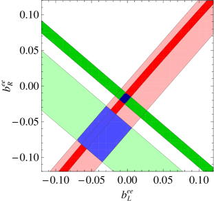
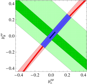
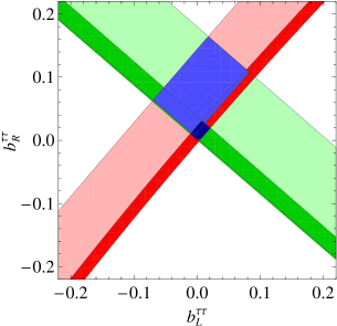
Figure 2: Values of $b_{L,R}^{ll}$ for  $m_{Z^{\prime}}=150$ GeV  and mixing angle  $\xi=0.008$ (lighter colors), $0.038$ (darker colors),  as described in the text, subject to constraints from $A_{l}$ and $\Gamma_{Z\to l^{+}l^{-}}$ data.

Applying  $\beta_{L,R}^{ll}=g_{L,R}/c_{\xi}+t_{\xi}\,b_{L,R}^{ll}$  from Eq. (21) in the $A_{l}$ and $\Gamma_{Z\to l^{+}l^{-}}$ formulas above, with  $g_{L,R}=g_{L,R}^{\rm eff}$  from Eq. (31) and a specific value of $\xi$, one can then obtain the allowed ranges of $b_{L,R}^{ll}$ from the measured values in Eq. (III) within their one-sigma ranges. Thus in the  $m_{Z^{\prime}}=150$ GeV  case, for which  $0.008\leq|\xi|\leq 0.038$,  the results for  $\xi>0$  are

$$-0.071\,\,\leq\,\,b_{L}^{ee}\,\,\leq\,\,0.006~{},\hskip 21.52771pt-0.11\,\,\leq\,\,b_{R}^{ee}\,\,\leq\,\,-0.009~{},$$ (32)

$$-0.13\,\,\leq\,\,b_{L}^{\mu\mu}\,\,\leq\,\,0.25~{},\hskip 21.52771pt-0.15\,\,\leq\,\,b_{R}^{\mu\mu}\,\,\leq\,\,0.27~{},$$

$$-0.070\,\,\leq\,\,b_{L}^{\tau\tau}\,\,\leq\,\,0.083~{},\hskip 21.52771pt-0.002\,\,\leq\,\,b_{R}^{\tau\tau}\,\,\leq\,\,0.16~{}.$$

Flipping the sign of $\xi$ would also flip the signs of these $b_{L,R}^{ll}$ numbers, and the same statement applies to the rest of our analysis. The plots in Fig. 2 illustrate the allowed $b_{L,R}^{ll}$ regions for the lower and upper limits of the $\xi$ range in this case,  $\xi=0.008$ (lighter colors) and  $\xi=0.038$ (darker colors).  The green regions satisfy the $A_{l}$ constraints, red the $\Gamma_{Z\to l^{+}l^{-}}$ constraints, and blue both of them. The upper and lower limits of the $b_{L,R}^{ll}$ ranges in Eq. (32) are visible on the plots.

Since $Z^{\prime}$-mediated diagrams can also affect the collision  $e^{+}e^{-}\to l^{+}l^{-}$,  it is important to consider the relevant data to see if they offer additional restraints on the $Z^{\prime}$ couplings. Here we will employ LEP-II measurements at various center-of-mass energies above the $Z$ pole, from 130 to 207 GeV  Alcaraz:2006mx . The amplitude for this process if  $l\neq e$  is

$${\cal M}_{e^{+}e^{-}\to\bar{l}l} = -\frac{e_{p}^{2}\,\bar{l}\gamma^{\nu}l\,\bar{e}\gamma_{\nu}e}{s}\,+\,\frac{\bar{l}\gamma^{\nu}\bigl{(}\beta_{L}^{ll}P_{L}+\beta_{R}^{ll}P_{R}\bigr{)}l\,\bar{e}\gamma_{\nu}\bigl{(}\beta_{L}^{ee}P_{L}+\beta_{R}^{ee}P_{R}\bigr{)}e}{m_{Z}^{2}-s}$$ (33)

$$\!+\;\frac{\bar{l}\gamma^{\nu}\bigl{(}b_{L}^{ll}P_{L}+b_{R}^{ll}P_{R}\bigr{)}l\,\bar{e}\gamma_{\nu}\bigl{(}b_{L}^{ee}P_{L}+b_{R}^{ee}P_{R}\bigr{)}e}{m_{Z^{\prime}}^{2}-s}~{},$$

where  $e_{p}>0$  is the proton’s electric charge,  $s=(p_{e^{+}}+p_{e^{-}})^{2}$,  and we have assumed that $s$ is not near $m_{Z,Z^{\prime}}^{2}$. There are also contributions to this amplitude from $t$-channel diagrams with flavor-changing couplings $\beta_{L,R}^{el}$ and $b_{L,R}^{el}$, but we will neglect their effects in order to explore the largest impact of the $Z^{\prime}$ flavor-conserving couplings under the assumption that there is no unnatural cancellation between the two sets of contributions. Moreover, as we demonstrate below, the magnitudes of the latter couplings have looser upper-limits than their flavor-changing counterparts by at least a few times. Complete expressions for the cross-section $\sigma(e^{+}e^{-}\to l^{+}l^{-})$ and forward-backward asymmetry $A_{\rm FB}$, including finite-width effects, are collected in Appendix B. Numerically, we adopt the couplings in Eq. (31) and the effective value  $\alpha=1/132$,  which in the absence of the $Z^{\prime}$ lead to $\sigma$ and $A_{\rm FB}$ numbers differing by no more than 2 percent from the corresponding SM predictions quoted in the LEP-II report Alcaraz:2006mx . Since we consider  $m_{Z^{\prime}}=150$ GeV and larger masses from 0.5 to 2 TeV,  in determining the $g_{L,R}^{ll}$ bounds we take the LEP-II data belonging to  $\sqrt{s}=136,161,205,207$ GeV  for definiteness.

We find that incorporating the LEP-II information brings about significant modifications to some of the results in Eq. (32). The allowed values of the couplings for  $m_{Z^{\prime}}=150$ GeV  now become

$$-0.071\,\,\leq\,\,b_{L}^{ee}\,\,\leq\,\,0.006~{},\hskip 21.52771pt-0.10\,\,\leq\,\,b_{R}^{ee}\,\,\leq\,\,-0.009~{},$$ (34)

$$-0.033\,\,\leq\,\,b_{L}^{\mu\mu}\,\,\leq\,\,0.080~{},\hskip 21.52771pt-0.029\,\,\leq\,\,b_{R}^{\mu\mu}\,\,\leq\,\,0.095~{},$$

$$-0.070\,\,\leq\,\,b_{L}^{\tau\tau}\,\,\leq\,\,0.024~{},\hskip 43.05542pt0\,\,\leq\,\,b_{R}^{\tau\tau}\,\,\leq\,\,0.083~{}.$$

We have also explored the situations for higher masses up to  $m_{Z^{\prime}}=2$ TeV.  The inclusion of the LEP-II data again provide important extra restrictions on the couplings. For the representative values  $m_{Z^{\prime}}=0.5$ - 2 TeV,  the allowed ranges associated with each flavor turn out to be roughly proportional to the $m_{Z^{\prime}}$ values, namely

$$\displaystyle-5.1\,\,\lesssim\,\,\frac{b_{L}^{ee}}{m_{Z^{\prime}}}\,\,\lesssim\,\,-1.2~{},\hskip 21.52771pt-5.4\,\,\lesssim\,\,\frac{b_{R}^{ee}}{m_{Z^{\prime}}}\,\,\lesssim\,\,-1.1~{},$$ (35)

$$\displaystyle-4.3\,\,\lesssim\,\,\frac{b_{L}^{\mu\mu}}{m_{Z^{\prime}}}\,\,\lesssim\,\,3.4~{},\hskip 27.98602pt-4.3\,\,\lesssim\,\,\frac{b_{R}^{\mu\mu}}{m_{Z^{\prime}}}\,\,\lesssim\,\,2.1~{},$$

$$\displaystyle-6.1\,\,\lesssim\,\,\frac{b_{L}^{\tau\tau}}{m_{Z^{\prime}}}\,\,\lesssim\,\,-2.0~{},\hskip 30.1388pt1.9\,\,\lesssim\,\,\frac{b_{R}^{\tau\tau}}{m_{Z^{\prime}}}\,\,\lesssim\,\,5.9~{},$$

where the numbers are in units of  $10^{-4}$ GeV^-1.  In obtaining all the $b_{L,R}^{ll}$ ranges above, we let the couplings be present at the same time. It is worth noting that the proportionality of these ranges to the $Z^{\prime}$ mass for  $m_{Z^{\prime}}\gg m_{Z}$  is a reflection of the  $|$$\tan\xi|\propto 1/m_{Z^{\prime}}$  behavior in Eq. (25) which starts to manifest itself when $m_{Z^{\prime}}$ exceeds 200 GeV or so, as can be seen in Fig. 1. We also note that for  $m_{Z^{\prime}}\,{\scriptstyle\gtrsim}\,2$ TeV  the limits in Eq. (35) accommodate couplings which may exceed order one in magnitude and hence the perturbativity limit. Nevertheless, as the errors in $\rho_{0}$ decrease with increasingly better precision in future data, the bounds on $b_{L,R}^{ll}$ will likely become stronger.

Before proceeding to the flavor-changing sector, a few comments regarding the case of no $Z$-$Z^{\prime}$ mixing,  $\xi=0$,  are in order. If one goes beyond the one-sigma range of the $\rho_{0}$ parameter from the global electroweak fit, so that the lower bound of $\rho_{0}$ reaches zero, then the lower bound of $|\xi|$ will also reach zero. In that limit  $\beta_{L,R}^{ll}\to g_{L,R}$,  and therefore the $Z$-pole data on $A_{l}$ and $\Gamma_{Z\to l^{+}l^{-}}$ no longer offer restrictions on $b_{L,R}^{ll}$ through the tree-level relations in Eqs. (27) and (28). At the one-loop level, however, $Z^{\prime}$-mediated radiative corrections contribute to the $Zl^{+}l^{-}$ vertex, and so these observables can still constrain the couplings Carone:1994aa . With the formulas given in Ref. Carone:1994aa for the $Z^{\prime}$-loop contribution, we estimate that the upper limits on the coupling-to-mass ratios, $b/m_{Z^{\prime}}$, are of order 1 to 2 per mill GeV^-1 for our $m_{Z^{\prime}}$ range of interest and thus higher than their counterparts in the presence of mixing. Without the mixing, $Z^{\prime}$-mediated diagrams can still affect  $e^{+}e^{-}\to l^{+}l^{-}$  at tree level, as Eq. (33) indicates. The expressions for the cross section and forward-backward asymmetry in Appendix B suggest, however, that the LEP-II data would not impose additional restrictions in this case.

IV Constraints from tree-level flavor-changing processes

IV.1 $\bm{Z\to e^{\pm}\mu^{\mp}}$,  $\bm{Z\to e^{\pm}\tau^{\mp}}$,  and  $\bm{Z\to\mu^{\pm}\tau^{\mp}}$

As ${\cal L}_{\rm int}$ in Eq. (19) shows, the $Z$ can have tree-level flavor-violating interactions with leptons in the presence of $Z$-$Z^{\prime}$ mixing. Accordingly, the amplitude of the decay  $Z\to l\bar{l}^{\prime}$  for  $l^{\prime}\neq l$  is

$${\cal M}_{Z\to l\bar{l}^{\prime}}\,\,=\,\,\bar{l}\gamma_{\lambda}\bigl{(}\beta_{L}^{ll^{\prime}}P_{L}+\beta_{R}^{ll^{\prime}}P_{R}\bigr{)}l^{\prime}\,\varepsilon_{Z}^{\lambda}~{},$$ (36)

where  $\beta_{L,R}^{ll^{\prime}}=t_{\xi}\,b_{L,R}^{ll^{\prime}}$  from Eq. (21). The rate of this transition is then

$$\Gamma_{Z\to l\bar{l}^{\prime}}\,\,=\,\,\frac{|\bm{p}_{l}|\,t_{\xi}^{2}}{8\pi m_{Z}^{2}}\Biggl{\{}\!\Bigl{(}\bigl{|}b_{L}^{ll^{\prime}\!}\bigr{|}^{2}+\bigl{|}b_{R}^{ll^{\prime}\!}\bigr{|}^{2}\Bigr{)}\Biggl{[}\frac{2m_{Z}^{2}-m_{l}^{2}-m_{l^{\prime}}^{2}}{3}-\frac{(m_{l}^{2}-m_{l^{\prime}}^{2})^{2}}{3m_{Z}^{2}}\Biggr{]}+4m_{l}m_{l^{\prime}}\,{\rm Re}\bigl{(}b_{L}^{ll^{\prime}\!*}b_{R}^{ll^{\prime}}\bigr{)}\biggr{\}}\,,~{}~{}~{}$$ (37)

where $\bm{p}_{l}$ is the three-momentum of $l$ in the $Z$ rest-frame. These decays, like all other lepton-flavor-violating ones, have not yet been observed. But there is some experimental information available on the branching ratios:  ${\cal B}(Z\to e^{\pm}\mu^{\mp})<1.7\times 10^{-6}$,   ${\cal B}(Z\to e^{\pm}\tau^{\mp})<9.8\times 10^{-6}$,  and  ${\cal B}(Z\to\mu^{\pm}\tau^{\mp})<1.2\times 10^{-5}$  pdg , each of the numbers being the sum of contributions from the listed final states. Assuming that only one of $\beta_{L,R}^{ll^{\prime}}$ is nonzero at a time, we can then obtain constraints on $b_{L,R}^{ll^{\prime}}$ after specifying $\xi$ associated with a given $Z^{\prime}$ mass. Thus for  $m_{Z^{\prime}}=150$ GeV,  in which case  $0.008\leq|\xi|\leq 0.038$,

$$\bigl{|}b_{L,R}^{e\mu}\bigr{|}\,\,\leq\,\,0.17~{},\hskip 21.52771pt\bigl{|}b_{L,R}^{e\tau}\bigr{|}\,\,\leq\,\,0.41~{},\hskip 21.52771pt\bigl{|}b_{L,R}^{\mu\tau}\bigr{|}\,\,\leq\,\,0.44~{}.$$ (38)

For the higher masses,  $m_{Z^{\prime}}=0.5$ - 2 TeV,  we find that the upper bounds are again approximately proportional to their masses,

$$\frac{\bigl{|}b_{L,R}^{e\mu}\bigr{|}}{m_{Z^{\prime}}}\,\,\lesssim\,\,1.4~{},\hskip 21.52771pt\frac{\bigl{|}b_{L,R}^{e\tau}\bigr{|}}{m_{Z^{\prime}}}\,\,\lesssim\,\,3.5~{},\hskip 21.52771pt\frac{\bigl{|}b_{L,R}^{\mu\tau}\bigr{|}}{m_{Z^{\prime}}}\,\,\lesssim\,\,3.8$$ (39)

in units of  $10^{-3}$ GeV^-1.  Stricter constraints can come from some of the other processes we study in the following.

IV.2 $\bm{\mu\to 3e}$,  $\bm{\tau\to 3e}$,  and  $\bm{\tau\to 3\mu}$

The decay  $\mu^{-}\to e^{-}e^{+}e^{-}$  receives contributions from diagrams involving the $Z$ and $Z^{\prime}$. From ${\cal L}_{\rm int}$ in Eq. (19), we derive the amplitude for the tree-level contributions to be

$${\cal M}_{\mu\to 3e} = \biggl{(}\frac{\beta_{L}^{ee}\beta_{L}^{e\mu}}{m_{Z}^{2}}+\frac{b_{L}^{ee}b_{L}^{e\mu}}{m_{Z^{\prime}}^{2}}\biggr{)}\bar{e}\gamma^{\nu}P_{L}e\,\bar{e}^{\prime}\gamma_{\nu}P_{L}\mu+\biggl{(}\frac{\beta_{R}^{ee}\beta_{R}^{e\mu}}{m_{Z}^{2}}+\frac{b_{R}^{ee}b_{R}^{e\mu}}{m_{Z^{\prime}}^{2}}\biggr{)}\bar{e}\gamma^{\nu}P_{R}e\,\bar{e}^{\prime}\gamma_{\nu}P_{R}\mu$$ (40)

$$\!+\;\biggl{(}\frac{\beta_{L}^{ee}\beta_{R}^{e\mu}}{m_{Z}^{2}}+\frac{b_{L}^{ee}b_{R}^{e\mu}}{m_{Z^{\prime}}^{2}}\biggr{)}\bar{e}\gamma^{\nu}P_{L}e\,\bar{e}^{\prime}\gamma_{\nu}P_{R}\mu+\biggl{(}\frac{\beta_{R}^{ee}\beta_{L}^{e\mu}}{m_{Z}^{2}}+\frac{b_{R}^{ee}b_{L}^{e\mu}}{m_{Z^{\prime}}^{2}}\biggr{)}\bar{e}\gamma^{\nu}P_{R}e\,\bar{e}^{\prime}\gamma_{\nu}P_{L}\mu$$

$$\!-\;\bigl{(}\bar{e}\leftrightarrow\bar{e}^{\prime}\bigr{)}~{}.$$

Here we use $\bar{e}$ and $\bar{e}^{\prime}$ to distinguish the two electrons in the final state. The minus sign in the above equation comes from Fermi statistics. Using  $\beta_{L,R}^{e\mu}=t_{\xi}b_{L,R}^{e\mu}$  and ignoring the electron mass, we can write the resulting branching ratio as

$${\cal B}(\mu\to 3e) = \frac{\tau_{\mu}\,m_{\mu}^{5}}{1536\,\pi^{3}}\Biggl{\{}\Biggl{[}2\biggl{(}\frac{t_{\xi}\beta_{L}^{ee}}{m_{Z}^{2}}+\frac{b_{L}^{ee}}{m_{Z^{\prime}}^{2}}\biggr{)}^{\!\!2}\!+\biggl{(}\frac{t_{\xi}\beta_{R}^{ee}}{m_{Z}^{2}}+\frac{b_{R}^{ee}}{m_{Z^{\prime}}^{2}}\biggr{)}^{\!\!2}\Biggr{]}\bigl{|}b_{L}^{e\mu}\bigr{|}^{2}$$ (41)

$$\hskip 38.74988pt+\;\Biggl{[}\biggl{(}\frac{t_{\xi}\beta_{L}^{ee}}{m_{Z}^{2}}+\frac{b_{L}^{ee}}{m_{Z^{\prime}}^{2}}\biggr{)}^{\!\!2}\!+2\biggl{(}\frac{t_{\xi}\beta_{R}^{ee}}{m_{Z}^{2}}+\frac{b_{R}^{ee}}{m_{Z^{\prime}}^{2}}\biggr{)}^{\!\!2}\Biggr{]}\bigl{|}b_{R}^{e\mu}\bigr{|}^{2}\Biggr{\}}~{},$$

where $\tau_{\mu}$ is the $\mu$ lifetime and  $\beta_{L,R}^{ee}=g_{L,R}/c_{\xi}+t_{\xi}\,b_{L,R}^{ee}$.

To evaluate the upper limits on $|b_{L,R}^{e\mu}|{}^{2}$ from the data on  $\mu\to 3e$,  one can try to look for nonzero minima of the coefficients of $|b_{L,R}^{e\mu}|^{2}$ in the ${\cal B}(\mu\to 3e)$ formula. After scanning the values of $\xi$ and $b_{L,R}^{ee}$ satisfying the experimental requirements discussed in the previous section, we find for  $m_{Z^{\prime}}=150$ GeV  that the minimum of the coefficient of  $|b_{L}^{e\mu}|{}^{2}$  is  $4.7\times 10^{-4}$  at  $\bigl{(}b_{L}^{ee},b_{R}^{ee},\xi\bigr{)}\simeq\pm(0.0042,-0.021,0.025)$,  whereas that of  $|b_{R}^{e\mu}|{}^{2}$  is  $3.1\times 10^{-4}$  at  $\bigl{(}b_{L}^{ee},b_{R}^{ee},\xi\bigr{)}\simeq\pm(0.0045,-0.018,0.031)$.  From the measured bound  ${\cal B}(\mu^{-}\to e^{-}e^{+}e^{-})_{\rm exp}<1.0\times 10^{-12}$  pdg , assuming as before that only one of $\beta_{L,R}^{e\mu}$ is nonvanishing at a time, we then extract in the  $m_{Z^{\prime}}=150$ GeV  case

$$\bigl{|}b_{L}^{e\mu}\bigr{|}\,\,\leq\,\,4.6\times 10^{-5}~{},\hskip 21.52771pt\bigl{|}b_{R}^{e\mu}\bigr{|}\,\,\leq\,\,5.7\times 10^{-5}~{}.$$ (42)

For  $m_{Z^{\prime}}=0.5$ - 2 TeV,  taking similar steps we obtain the limits to be roughly proportional to $m_{Z^{\prime}}$ according to

$$\frac{\bigl{|}b_{L}^{e\mu}\bigr{|}}{m_{Z^{\prime}}}\,\,\lesssim\,\,1.4\times 10^{-7}{\rm~{}GeV}^{-1}~{},\hskip 21.52771pt\frac{\bigl{|}b_{R}^{e\mu}\bigr{|}}{m_{Z^{\prime}}}\,\,\lesssim\,\,1.8\times 10^{-7}{\rm~{}GeV}^{-1}~{}.$$ (43)

In the analogous case of  $\tau^{-}\to e^{-}e^{+}e^{-}$,  the expression for the branching ratio can be simply derived from that for  ${\cal B}(\mu\to 3e)$  by replacing each $\mu$ in the indices with $\tau$. The same can be said about the coefficients of $\bigl{|}b_{L,R}^{e\tau}\bigr{|}{}^{2}$ in the ${\cal B}(\tau\to 3e)$ formula. It follows that the measured bound  ${\cal B}(\tau^{-}\to e^{-}e^{+}e^{-})_{\rm exp}<2.7\times 10^{-8}$  pdg yields for  $m_{Z^{\prime}}=150$ GeV

$$\bigl{|}b_{L}^{e\tau}\bigr{|}\,\,\leq\,\,0.018~{},\hskip 21.52771pt\bigl{|}b_{R}^{e\tau}\bigr{|}\,\,\leq\,\,0.022~{},$$ (44)

whereas for  $m_{Z^{\prime}}=0.5$ - 2 TeV

$$\frac{\bigl{|}b_{L}^{e\tau}\bigr{|}}{m_{Z^{\prime}}}\,\,\lesssim\,\,5.3\times 10^{-5}{\rm~{}GeV}^{-1}~{},\hskip 21.52771pt\frac{\bigl{|}b_{R}^{e\tau}\bigr{|}}{m_{Z^{\prime}}}\,\,\lesssim\,\,6.9\times 10^{-5}{\rm~{}GeV}^{-1}~{}.$$ (45)

As for  $\tau^{-}\to\mu^{-}\mu^{+}\mu^{-}$,  upon scanning the allowed values of $b_{L,R}^{\mu\mu}$ and $\xi$ we find that the coefficients of $\bigl{|}b_{L,R}^{\mu\tau}\bigr{|}{}^{2}$ in the ${\cal B}(\tau\to 3\mu)$ formula have minima which are vanishingly small. Consequently, this mode cannot provide useful restraints on $\bigl{|}b_{L,R}^{\mu\tau}\bigr{|}$ separately.

IV.3 $\bm{\tau\to\mu\bar{e}e}$  and  $\bm{\tau\to e\bar{\mu}\mu}$

Another transition that can happen in our $Z^{\prime}$ scenario is  $\tau^{-}\to\mu^{-}e^{+}e^{-}$.  The tree-level contribution to its amplitude is

$${\cal M}_{\tau\to\mu\bar{e}e} = \biggl{(}\frac{\beta_{L}^{ee}\beta_{L}^{\mu\tau}}{m_{Z}^{2}}+\frac{b_{L}^{ee}b_{L}^{\mu\tau}}{m_{Z^{\prime}}^{2}}\biggr{)}\bar{e}\gamma^{\nu}P_{L}e\,\bar{\mu}\gamma_{\nu}P_{L}\tau+\biggl{(}\frac{\beta_{L}^{ee}\beta_{R}^{\mu\tau}}{m_{Z}^{2}}+\frac{b_{L}^{ee}b_{R}^{\mu\tau}}{m_{Z^{\prime}}^{2}}\biggr{)}\bar{e}\gamma^{\nu}P_{L}e\,\bar{\mu}\gamma_{\nu}P_{R}\tau$$ (46)

$$\!-\;\biggl{(}\frac{\beta_{L}^{\mu e}\beta_{L}^{e\tau}}{m_{Z}^{2}}+\frac{b_{L}^{\mu e}b_{L}^{e\tau}}{m_{Z^{\prime}}^{2}}\biggr{)}\bar{\mu}\gamma^{\nu}P_{L}e\,\bar{e}\gamma_{\nu}P_{L}\tau-\biggl{(}\frac{\beta_{L}^{\mu e}\beta_{R}^{e\tau}}{m_{Z}^{2}}+\frac{b_{L}^{\mu e}b_{R}^{e\tau}}{m_{Z^{\prime}}^{2}}\biggr{)}\bar{\mu}\gamma^{\nu}P_{L}e\,\bar{e}\gamma_{\nu}P_{R}\tau$$

$$\!+\;(L\leftrightarrow R)~{}.$$

It leads to the branching ratio

$${\cal B}(\tau\to\mu\bar{e}e) = \frac{\tau_{\tau}\,m_{\tau}^{5}}{1536\pi^{3}}\Biggl{[}\biggl{|}\biggl{(}\frac{t_{\xi}\beta_{L}^{ee}}{m_{Z}^{2}}+\frac{b_{L}^{ee}}{m_{Z^{\prime}}^{2}}\biggr{)}b_{L}^{\mu\tau}+\frac{b_{L}^{\mu e}b_{L}^{e\tau}}{m_{Z^{\prime}}^{2}}\biggr{|}^{2}+\biggl{|}\biggl{(}\frac{t_{\xi}\beta_{R}^{ee}}{m_{Z}^{2}}+\frac{b_{R}^{ee}}{m_{Z^{\prime}}^{2}}\biggr{)}b_{R}^{\mu\tau}+\frac{b_{R}^{\mu e}b_{R}^{e\tau}}{m_{Z^{\prime}}^{2}}\biggr{|}^{2}$$

$$\hskip 34.44434pt+\,\biggl{(}\frac{t_{\xi}\beta_{L}^{ee}}{m_{Z}^{2}}+\frac{b_{L}^{ee}}{m_{Z^{\prime}}^{2}}\biggr{)}^{\!\!2}|b_{R}^{\mu\tau}|^{2}+\biggl{(}\frac{t_{\xi}\beta_{R}^{ee}}{m_{Z}^{2}}+\frac{b_{R}^{ee}}{m_{Z^{\prime}}^{2}}\biggr{)}^{\!\!2}|b_{L}^{\mu\tau}|^{2}+\frac{|b_{L}^{\mu e}b_{R}^{e\tau}|^{2}+|b_{R}^{\mu e}b_{L}^{e\tau}|^{2}}{m_{Z^{\prime}}^{2}}\Biggr{]},$$

where final lepton masses have been neglected and terms containing  $\bigl{|}\beta_{\sf C}^{\mu e}\beta_{\sf C^{\prime}}^{e\tau}\bigr{|}=t_{\xi}^{2}\bigl{|}b_{\sf C}^{\mu e}b_{\sf C^{\prime}}^{e\tau}\bigr{|}$  for  ${\sf C,C^{\prime}}=L,R$  have been dropped because  $t_{\xi}^{2}\ll m_{Z}^{2}/m_{Z^{\prime}}^{2}$.  To determine the upper bounds on  $|b_{L,R}^{\mu\tau}|^{2}$,  one can again then try to seek nonvanishing minima of their coefficients in Eq. (IV.3) which are the same, under the assumption that $b_{\sf C}^{\mu e,e\tau}$ are absent. Thus for  $m_{Z^{\prime}}=150$ GeV  we place the minimum to be  $4.9\times 10^{-5}$  at  $\bigl{(}b_{L}^{ee},b_{R}^{ee},\xi\bigr{)}\simeq\pm(0.0043,-0.019,0.028)$.  From the experimental information  ${\cal B}(\tau^{-}\to\mu^{-}e^{+}e^{-})_{\rm exp}<1.8\times 10^{-8}$  pdg , we subsequently extract for  $m_{Z^{\prime}}=150$ GeV

$$\bigl{|}b_{L,R}^{\mu\tau}\bigr{|}\,\,\leq\,\,0.019~{}.$$ (48)

Similarly, for  $m_{Z^{\prime}}=0.5$ - 2 TeV  we arrive at

$$\frac{\bigl{|}b_{L,R}^{\mu\tau}\bigr{|}}{m_{Z^{\prime}}}\,\,\lesssim\,\,6\times 10^{-5}{\rm~{}GeV}^{-1}~{}.$$ (49)

Assuming  $b_{L,R}^{\mu\tau}=0$  instead, we get

$$\frac{\bigl{|}b_{\sf C}^{\mu e}b_{\sf C^{\prime}}^{e\tau}\bigr{|}}{m_{Z^{\prime}}^{2}}\,\,\leq\,\,1.0\times 10^{-8}{\rm~{}GeV}^{-2}~{}.$$ (50)

The constraints in the last equation are weaker by  $\sim$3  orders of magnitude than those put together from Eqs. (42)-(45).

For  $\tau^{-}\to e^{-}\mu^{+}\mu^{-}$,  the expression for the branching ratio follows from that for  ${\cal B}(\tau\to\mu\bar{e}e)$  with $e$ and $\mu$ being interchanged in the indices. In this case the coefficients of $\bigl{|}b_{L,R}^{e\tau}\bigr{|}{}^{2}$ in  ${\cal B}(\tau\to e\bar{\mu}\mu)$  have vanishingly small minima. Hence useful upper-bounds on these couplings are not available from  ${\cal B}(\tau^{-}\to e^{-}\mu^{+}\mu^{-})_{\rm exp}<2.7\times 10^{-8}$  pdg . On the other hand, assuming  $b_{L,R}^{e\tau}=0$  we can extract

$$\frac{\bigl{|}b_{\sf C}^{e\mu}b_{\sf C^{\prime}}^{\mu\tau}\bigr{|}}{m_{Z^{\prime}}^{2}}\,\,\leq\,\,1.3\times 10^{-8}{\rm~{}GeV}^{-2}~{},$$ (51)

which are also very weak compared to what can be deduced from Eqs. (43) and (49).

IV.4 $\bm{\tau\to ee\bar{\mu}}$  and  $\bm{\tau\to\bar{e}\mu\mu}$

Like the preceding ones, the  $\tau^{-}\to e^{-}e^{-}\mu^{+}$  decay receives tree-level contributions proceeding from Eq. (19), but involves two flavor-changing vertices exclusively. The amplitude is given by

$${\cal M}_{\tau\to ee\bar{\mu}} = \biggl{(}\frac{\beta_{L}^{e\mu}\beta_{L}^{e\tau}}{m_{Z}^{2}}+\frac{b_{L}^{e\mu}b_{L}^{e\tau}}{m_{Z^{\prime}}^{2}}\biggr{)}\bar{e}\gamma^{\nu}P_{L}\mu\,\bar{e}^{\prime}\gamma_{\nu}P_{L}\tau+\biggl{(}\frac{\beta_{R}^{e\mu}\beta_{R}^{e\tau}}{m_{Z}^{2}}+\frac{b_{R}^{e\mu}b_{R}^{e\tau}}{m_{Z^{\prime}}^{2}}\biggr{)}\bar{e}\gamma^{\nu}P_{R}\mu\,\bar{e}^{\prime}\gamma_{\nu}P_{R}\tau$$ (52)

$$\!+\;\biggl{(}\frac{\beta_{L}^{e\mu}\beta_{R}^{e\tau}}{m_{Z}^{2}}+\frac{b_{L}^{e\mu}b_{R}^{e\tau}}{m_{Z^{\prime}}^{2}}\biggr{)}\bar{e}\gamma^{\nu}P_{L}\mu\,\bar{e}^{\prime}\gamma_{\nu}P_{R}\tau+\biggl{(}\frac{\beta_{R}^{e\mu}\beta_{L}^{e\tau}}{m_{Z}^{2}}+\frac{b_{R}^{e\mu}b_{L}^{e\tau}}{m_{Z^{\prime}}^{2}}\biggr{)}\bar{e}\gamma^{\nu}P_{R}\mu\,\bar{e}^{\prime}\gamma_{\nu}P_{L}\tau$$

$$\!-\;\bigl{(}\bar{e}\leftrightarrow\bar{e}^{\prime}\bigr{)}~{}.$$

Neglecting the terms involving  $\beta_{\sf C}^{e\mu}\beta_{\sf C^{\prime}}^{e\tau}$  as before, we consequently have

$${\cal B}(\tau\to ee\bar{\mu}) = \frac{\tau_{\tau}\,m_{\tau}^{5}}{1536\,\pi^{3}}\Biggl{(}\frac{2|b_{L}^{e\mu}|^{2}+|b_{R}^{e\mu}|^{2}}{m_{Z^{\prime}}^{4}}\bigl{|}b_{L}^{e\tau}\bigr{|}^{2}+\frac{|b_{L}^{e\mu}|^{2}+2|b_{R}^{e\mu}|^{2}}{m_{Z^{\prime}}^{4}}\bigl{|}b_{R}^{e\mu}\bigr{|}^{2}\Biggr{)}~{}.$$ (53)

The measurement  ${\cal B}(\tau^{-}\to\mu^{+}e^{-}e^{-})_{\rm exp}<1.5\times 10^{-8}$  pdg then implies

$$\frac{\bigl{|}{b}_{L,R}^{e\mu}{b}_{L,R}^{e\tau}\bigr{|}}{m_{Z^{\prime}}^{2}}\,\,\leq\,\,6.8\times 10^{-9}~{}\mbox{GeV}^{-2}~{},\hskip 21.52771pt\frac{\bigl{|}{b}_{L,R}^{e\mu}{b}_{R,L}^{e\tau}\bigr{|}}{m_{Z^{\prime}}^{2}}\,\,\leq\,\,9.6\times 10^{-9}~{}\mbox{GeV}^{-2}~{}.$$ (54)

For  $\tau^{-}\to e^{+}\mu^{-}\mu^{-}$,  following analogous steps we obtain from  ${\cal B}(\tau^{-}\to e^{+}\mu^{-}\mu^{-})_{\rm exp}<1.7\times 10^{-8}$  pdg that

$$\frac{\bigl{|}{b}_{L,R}^{\mu e}{b}_{L,R}^{\mu\tau}\bigr{|}}{m_{Z^{\prime}}^{2}}\,\,\leq\,\,7.2\times 10^{-9}~{}\mbox{GeV}^{-2}~{},\hskip 21.52771pt\frac{\bigl{|}{b}_{L,R}^{\mu e}{b}_{R,L}^{\mu\tau}\bigr{|}}{m_{Z^{\prime}}^{2}}\,\,\leq\,\,1.0\times 10^{-8}~{}\mbox{GeV}^{-2}~{}.$$ (55)

All these results are again less strict than the corresponding constraints inferred from Eqs. (43), (45), and (49) by roughly 3 orders of magnitude.

IV.5 Muonium-antimuonium conversion  $\bm{\mu^{+}e^{-}\to\mu^{-}e^{+}}$

The experimental information on  $\mu^{+}e^{-}\to\mu^{-}e^{+}$  is available in terms of the effective parameter $G_{C}$ which is defined by pdg ; Willmann:1998gd

$${\cal L}_{\rm eff}\,\,=\,\,\sqrt{8}\,G_{C}\,\bar{\mu}\gamma^{\nu}P_{\sf C^{\prime}\,}e\,\bar{\mu}\gamma_{\nu}P_{{\sf C}^{\prime}\,}e\;+\;{\rm H.c.}~{},$$ (56)

with  ${\sf C}^{\prime}=L$ or $R$,  and has been measured to be  $|G_{C}|<0.0030\,G_{\rm F}$ pdg , where $G_{\rm F}$ is the Fermi coupling constant. Attributing this to the $Z^{\prime}$ implies that

$$\frac{\bigl{|}b_{L,R}^{\mu e}\bigr{|}}{m_{Z^{\prime}}}\,\,=\,\,2\sqrt{\sqrt{2}\,|G_{C}|}\,\,\leq\,\,4.4\times 10^{-4}{\rm~{}GeV}^{-1}~{},$$ (57)

far less restrictive than Eq. (43).

IV.6 Flavor violating  $\bm{e^{+}e^{-}\to\bar{l}l^{\prime}}$

At  $e^{+}e^{-}$  colliders, new physics could trigger the production of flavor-violating events with $e\mu$, $e\tau$, and $\mu\tau$ in the final states. In our $Z^{\prime}$ scenario, the tree-level amplitude of  $e^{+}e^{-}\to l^{+}l^{\prime-}$  for  $l^{\prime}\neq l$  is

$${\cal M}_{\bar{e}e\to\bar{l}l^{\prime}} = \frac{\bar{l}^{\prime}\gamma^{\nu}\bigl{(}\beta_{L}^{l^{\prime}l}P_{L}+\beta_{R}^{l^{\prime}l}P_{R}\bigr{)}l\,\bar{e}\gamma_{\nu}\bigl{(}\beta_{L}^{ee}P_{L}+\beta_{R}^{ee}P_{R}\bigr{)}e}{m_{Z}^{2}-s}$$ (58)

$$-\;\frac{\bar{e}\gamma^{\nu}\bigl{(}\beta_{L}^{el}P_{L}+\beta_{R}^{el}P_{R}\bigr{)}l\,\bar{l}^{\prime}\gamma_{\nu}\bigl{(}\beta_{L}^{l^{\prime}e}P_{L}+\beta_{R}^{l^{\prime}e}P_{R}\bigr{)}e}{m_{Z}^{2}-t}$$

$$+\;\bigl{(}Z\to Z^{\prime},\,\beta\to b\bigr{)}~{},$$

where  $s=\bigl{(}p_{e^{+}}+p_{e^{-}}\bigr{)}{}^{2}$  is assumed not to be close to $m_{Z,Z^{\prime}}^{2}$ and  $t=\bigl{(}p_{e^{+}}-p_{l^{+}}\bigr{)}{}^{2}$.  The first experimental limits on the cross sections  $\sigma(ll^{\prime})\equiv\sigma(\bar{e}e\to\bar{l}l^{\prime})+\sigma(\bar{e}e\to l\bar{l}^{\prime})$  were acquired by the OPAL Collaboration Abbiendi:2001cs at LEP-II energies, ${\cal O}(200$ GeV).  More recent bounds on the cross sections at much lower energies, around  11 and 1 GeV,  were reported by the BaBar Aubert:2006uy and SND Achasov:2009en Collaborations, respectively. Since the theoretical cross sections tend to grow significantly as the energy increases from 1 to 200 GeV, the OPAL data Abbiendi:2001cs  $\bar{\sigma}(e\mu)_{\rm exp}<22$ fb,   $\bar{\sigma}(e\tau)_{\rm exp}<78$ fb,  and  $\bar{\sigma}(\mu\tau)_{\rm exp}<64$ fb  for the average cross sections over  $200{\rm\,GeV}\leq\sqrt{s}\leq 209$ GeV  impose potentially stronger restraints than the others. The cross sections at these energies being more sensitive to the effects of  $m_{Z^{\prime}}=150$ GeV  than to those of  $m_{Z^{\prime}}\geq 0.5$ TeV,  we discuss only the case of the former, in which for  $l=\mu$ or $\tau$

$$\bar{\sigma}(el) \simeq \bigl{[}38.4\,\bigl{(}\beta_{L}^{ee}\,t_{\xi}\bigr{)}{}^{2}+175\,\bigl{(}\beta_{R}^{ee}\,t_{\xi}\bigr{)}{}^{2}-20.9\,\beta_{L}^{ee}\,b_{L}^{ee}\,t_{\xi}+230\,\beta_{R}^{ee}\,b_{R}^{ee}\,t_{\xi}$$ (59)

$$~{}+\,9.68\,\bigl{(}b_{L}^{ee}\bigr{)}{}^{2}+103\,\bigl{(}b_{R}^{ee}\bigr{)}{}^{2}\bigr{]}\bigl{|}b_{L}^{le}\bigr{|}{}^{2}\times 10^{4}{\rm~{}fb}$$

$$+\;(L\leftrightarrow R)~{},$$

$$\vphantom{|^{\big{|}}}\bar{\sigma}(\mu\tau) \simeq \bigl{\{}\bigl{[}193\,\bigl{(}\beta_{L}^{ee}\,t_{\xi}\bigr{)}{}^{2}+669\,\beta_{L}^{ee}\,b_{L}^{ee}\,t_{\xi}+581\,\bigl{(}b_{L}^{ee}\bigr{)}{}^{2}\,+\,(L\leftrightarrow R)\bigr{]}\bigl{|}b_{L}^{\mu\tau}\bigr{|}{}^{2}$$ (60)

$$~{}-\,\bigl{(}413\,\beta_{L}^{ee}\,t_{\xi}+717\,b_{L}^{ee}\bigr{)}\,{\rm Re}\bigl{(}b_{L}^{e\mu}b_{L}^{\mu\tau}b_{L}^{\tau e}\bigr{)}\,+\,\bigl{(}233\,\bigl{|}b_{L}^{e\mu}\bigr{|}{}^{2}+448\,\bigl{|}b_{R}^{e\mu}\bigr{|}{}^{2}\bigr{)}\bigl{|}b_{L}^{\tau e}\bigr{|}{}^{2}\bigr{\}}\times 10^{3}{\rm~{}fb}$$

$$+\;(L\leftrightarrow R)~{}.~{}~{}~{}~{}$$

Minimizing the coefficients of $\bigl{|}b_{L,R}^{le}\bigr{|}{}^{2}$ in $\bar{\sigma}(el)$ and comparing the latter to their data then yields

$$\displaystyle\bigl{|}b_{L}^{\mu e}\bigr{|}\,\,<\,\,0.76~{},\hskip 21.52771pt\bigl{|}b_{R}^{\mu e}\bigr{|}\,\,<\,\,0.52~{},\hskip 21.52771pt\bigl{|}b_{L}^{\tau e}\bigr{|}\,\,<\,\,1.4~{},\hskip 21.52771pt\bigl{|}b_{R}^{\tau e}\bigr{|}\,\,<\,\,1.0~{}.$$ (61)

In an analogous way, $\bar{\sigma}(\mu\tau)$ in the absence of $b_{L,R}^{e\mu}$ gives  $\bigl{|}b_{L,R}^{\mu\tau}\bigr{|}\leq 1.2$,  whereas assuming  $b_{L,R}^{\mu\tau}=0$  instead leads to

$$\bigl{|}b_{L,R}^{e\mu}b_{L,R}^{\tau e}\bigr{|}\,\,\leq\,\,0.017~{},\hskip 21.52771pt\bigl{|}b_{L,R}^{e\mu}b_{R,L}^{\tau e}\bigr{|}\,\,\leq\,\,0.012~{}.$$ (62)

These are all weaker than their counterparts from Eqs. (42), (44), and (48) by 50 times or more.

V Constraints from loop-generated processes

V.1 $\bm{\mu\to e\gamma}$,  $\bm{\tau\to e\gamma}$,  and  $\bm{\tau\to\mu\gamma}$

The flavor-violating radiative decay  $l\to l^{\prime}\gamma$  occurs at the loop level, and its amplitude takes the general gauge-invariant form

$${\cal M}_{l\to l^{\prime}\gamma}\,\,=\,\,i\varepsilon_{\mu}^{*}k_{\nu}\,\bar{l}^{\prime}\bigl{(}\Sigma_{L}^{l^{\prime}l}P_{L}+\Sigma_{R}^{l^{\prime}l}P_{R}\bigr{)}\sigma^{\mu\nu}l~{},$$ (63)

where $k$ is the momentum of the outgoing photon, the parameters $\Sigma_{L,R}^{l^{\prime}l}$ depend on the loop contents, and  $\sigma^{\nu\omega}=\frac{i}{2}[\gamma^{\nu},\gamma^{\omega}]$.  This leads to the branching ratio

$${\cal B}(l\to l^{\prime}\gamma)\,\,=\,\,\frac{\tau_{l}\,\bigl{(}m_{l}^{2}-m_{l^{\prime}}^{2}\bigr{)}^{3}}{16\pi\,m_{l}^{3}}\Bigl{(}\bigl{|}\Sigma_{L}^{l^{\prime}l}\bigr{|}^{2}+\bigl{|}\Sigma_{R}^{l^{\prime}l}\bigr{|}^{2}\Bigr{)}~{},$$ (64)

where $\tau_{l}$ is the $l$ lifetime.

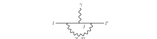
Figure 3: Diagram for $Z$ and $Z^{\prime}$ contributions to flavor-violating radiative decay  $l\to l^{\prime}\gamma$.

This decay receives $Z$- and $Z^{\prime}$-induced contributions via the diagram displayed in Fig. 3, with internal lepton $j$. Since the masses $m_{l,l^{\prime},j}$ of the external and internal leptons are small relative to $m_{Z,Z^{\prime}}$, it is a good approximation to retain only the lowest order terms in expanding the loop functions in terms of $m_{l,l^{\prime},j}/m_{Z,Z^{\prime}}$. In that limit, we can employ the results of Ref. He:2009rz to derive for negatively charged leptons

$$\Sigma_{L}^{l^{\prime}l}\,=\,\,\frac{e_{p}}{24\pi^{2}\,m_{Z}^{2}}\sum_{j}\bigl{(}3\beta_{R}^{l^{\prime}j}\beta_{L}^{jl}\,m_{j}-\beta_{L}^{l^{\prime}j}\beta_{L}^{jl}\,m_{l^{\prime}}-\beta_{R}^{l^{\prime}j}\beta_{R}^{jl}\,m_{l}\bigr{)}\;+\;\bigl{(}Z\to Z^{\prime},\,\beta\to b\bigr{)}~{},$$

$$\Sigma_{R}^{l^{\prime}l}\,=\,\,\frac{e_{p}}{24\pi^{2}\,m_{Z}^{2}}\sum_{j}\bigl{(}3\beta_{L}^{l^{\prime}j}\beta_{R}^{jl}\,m_{j}-\beta_{R}^{l^{\prime}j}\beta_{R}^{jl}\,m_{l^{\prime}}-\beta_{L}^{l^{\prime}j}\beta_{L}^{jl}\,m_{l}\bigr{)}\;+\;\bigl{(}Z\to Z^{\prime},\,\beta\to b\bigr{)}~{},$$ (65)

where the sum is over  $j=e,\mu,\tau$  and  $\beta_{L,R}^{jl}=\beta_{L,R}^{lj*}$.  Since  $m_{\tau}\simeq 17\,m_{\mu}\gg m_{e}$,  we consider only the most enhanced terms in $\Sigma_{L,R}^{l^{\prime}l}$, the ones proportional to $m_{\tau}$. Accordingly

$$\displaystyle\Sigma_{L}^{e\mu}\,\,=\,\,\frac{e_{p}\,m_{\tau}\,b_{R}^{e\tau}b_{L}^{\tau\mu}}{8\pi^{2}\,m_{Z^{\prime}}^{2}}~{},\hskip 21.52771pt\Sigma_{R}^{e\mu}\,\,=\,\,\frac{e_{p}\,m_{\tau}\,b_{L}^{e\tau}b_{R}^{\tau\mu}}{8\pi^{2}\,m_{Z^{\prime}}^{2}}~{},$$ (66)

$$\displaystyle\Sigma_{L}^{e\tau}\,\,=\,\,\frac{e_{p}\,m_{\tau}}{24\pi^{2}}\Biggl{[}\frac{\bigl{(}3\beta_{L}^{\tau\tau}-\beta_{R}^{\tau\tau}-\beta_{R}^{ee}\bigr{)}\beta_{R}^{e\tau}}{m_{Z}^{2}}+\frac{\bigl{(}3b_{L}^{\tau\tau}-b_{R}^{\tau\tau}-b_{R}^{ee}\bigr{)}b_{R}^{e\tau}-b_{R}^{e\mu}b_{R}^{\mu\tau}}{m_{Z^{\prime}}^{2}}\Biggr{]}~{},$$

$$\displaystyle\Sigma_{L}^{\mu\tau}\,\,=\,\,\frac{e_{p}\,m_{\tau}}{24\pi^{2}}\Biggl{[}\frac{\bigl{(}3\beta_{L}^{\tau\tau}-\beta_{R}^{\tau\tau}-\beta_{R}^{\mu\mu}\bigr{)}\beta_{R}^{\mu\tau}}{m_{Z}^{2}}+\frac{\bigl{(}3b_{L}^{\tau\tau}-b_{R}^{\tau\tau}-b_{R}^{\mu\mu}\bigr{)}b_{R}^{\mu\tau}-b_{R}^{\mu e}b_{R}^{e\tau}}{m_{Z^{\prime}}^{2}}\Biggr{]}~{},$$ (67)

and $\Sigma_{R}^{e\tau,\mu\tau}$ follow from $\Sigma_{L}^{e\tau,\mu\tau}$ with $L$ and $R$ interchanged, where we have also neglected terms with $\beta_{\sf C}^{e\mu}\beta_{\sf C}^{\mu\tau}$ $\bigl{(}\beta_{\sf C}^{\mu e}\beta_{\sf C}^{e\tau}\bigr{)}$ in $\Sigma_{\sf C}^{e\tau}$ $\bigl{(}\Sigma_{\sf C}^{\mu\tau}\bigr{)}$.

The newest information from recent searches for these modes is  ${\cal B}(\mu\to e\gamma)_{\rm exp}<2.4\times 10^{-12}$  reported by the MEG Collaboration Adam:2011ch . With the aid of Eqs. (64) and (66), it translates into

$$\frac{\bigl{|}b_{L,R}^{\mu\tau}{b}_{R,L}^{\tau e}\bigr{|}}{m_{Z^{\prime}}^{2}}\,\,\leq\,\,2.6\times 10^{-11}~{}.$$ (68)

These numbers are 2 orders of magnitude smaller than the corresponding ones combined from Eqs. (45) and (49) and therefore complement them.

The present bounds for the other 2 decays are not as strong,  ${\cal B}(\tau\to e\gamma)_{\rm exp}<3.3\times 10^{-8}$  and  ${\cal B}(\tau\to\mu\gamma)_{\rm exp}<4.4\times 10^{-8}$  from BaBar Aubert:2009tk ; pdg . Setting  $b_{L,R}^{e\mu}=0$  first, one can try to evaluate from these data the biggest $\bigl{|}b_{L,R}^{e\tau,\mu\tau}\bigr{|}$ by seeking the minima of their coefficients in the ${\cal B}(\tau\to e\gamma,\mu\gamma)$ formulas. Thus for  $m_{Z^{\prime}}=150$ GeV  the strongest limit we can come up with is  $\bigl{|}b_{L}^{e\tau}\bigr{|}<0.2$,  whereas for  $m_{Z^{\prime}}=0.5$ - 2 TeV  we get

$$\frac{\bigl{|}b_{L}^{e\tau}\bigr{|}}{m_{Z^{\prime}}}\,\,\lesssim\,\,3.3\times 10^{-4}~{}, \frac{\bigl{|}b_{R}^{e\tau}\bigr{|}}{m_{Z^{\prime}}}\,\,\lesssim\,\,5.5\times 10^{-4}~{},$$ (69)

$$\frac{\bigl{|}b_{L}^{\mu\tau}\bigr{|}}{m_{Z^{\prime}}}\,\,\lesssim\,\,5.9\times 10^{-4}~{}, \frac{\bigl{|}b_{R}^{\mu\tau}\bigr{|}}{m_{Z^{\prime}}}\,\,\lesssim\,\,7.4\times 10^{-4}~{},$$ (70)

all of which are less strong than the results in Eqs. (44), (45), and (49) by about an order of magnitude. Assuming  $b_{L,R}^{e\tau}=0$  and  $b_{L,R}^{\mu\tau}=0$  instead leads to, respectively,

$$\frac{\bigl{|}b_{L,R}^{e\mu}{b}_{R,L}^{\mu\tau}\bigr{|}}{m_{Z^{\prime}}^{2}}\,\,\leq\,\,3.6\times 10^{-7}~{},\hskip 21.52771pt\frac{\bigl{|}b_{L,R}^{\mu e}{b}_{R,L}^{e\tau}\bigr{|}}{m_{Z^{\prime}}^{2}}\,\,\leq\,\,4.2\times 10^{-7}~{},$$ (71)

which are very weak compared to the corresponding constraints deduced from Eqs. (43), (45), and (49)

We remark that these  $l\to l^{\prime}\gamma$  decays effected by the $Z$ and $Z^{\prime}$, plus additional loop-induced transitions  $l\to l^{\prime}\gamma^{*}$  whose amplitudes vanish for a real photon, also contribute to the flavor-changing decays  $l\to l^{\prime}\,\overline{l}{}^{\prime\prime}l^{\prime\prime}$.  However, due to the loop suppression they are less important than the tree-level contributions already discussed in Section IV.

V.2 Anomalous magnetic moments

The effective Lagrangian representing the anomalous magnetic moment $a_{l}$ and electric dipole moment $d_{l}$ of a negatively-charged lepton $l$ is

$${\cal L}_{l\bar{l}\gamma}\,\,=\,\,\bar{l}\biggl{(}\frac{e_{p}\,a_{l}}{4m_{l}}\,-\,\frac{i\,d_{l}}{2}\,\gamma_{5}\biggr{)}\sigma^{\nu\omega}l\,F_{\nu\omega}~{},$$ (72)

where  $F_{\nu\omega}=\partial_{\nu}A_{\omega}-\partial_{\omega}A_{\nu}$  is the photon field-strength tensor. Nonstandard effects of the $Z$ and $Z^{\prime}$ on $a_{l}$ and $d_{l}$ appear at one-loop level, arising from the same diagram as in Fig. 3, but with  $l^{\prime}=l$.  From Eqs. (63) and (V.1), we then arrive at the amplitude

$${\cal M}_{l\bar{l}\gamma} = \frac{ie_{p}\,\varepsilon_{\nu}^{*}k_{\omega}}{48\pi^{2}m_{Z}^{2}}\sum_{j}\bar{l}\Bigl{[}3\bigl{(}\beta_{L}^{lj}\beta_{R}^{jl}+\beta_{R}^{lj}\beta_{L}^{jl}\bigr{)}m_{j}-2\bigl{(}\bigl{|}\beta_{L}^{lj}\bigr{|}{}^{2}+\bigl{|}\beta_{R}^{lj}\bigr{|}{}^{2}\bigr{)}m_{l}+3\bigl{(}\beta_{L}^{lj}\beta_{R}^{jl}-\beta_{L}^{jl}\beta_{R}^{lj}\bigr{)}m_{j\,}\gamma_{5}\Bigr{]}\sigma^{\nu\omega}l$$ (73)

$$\!+\;\bigl{(}Z\to Z^{\prime},\,\beta\to b\bigr{)}~{},$$

where $k$ is outgoing. In view of Eq. (72), the terms without $\gamma_{5}$ yield

$$a_{l}^{Z^{\prime}} = \frac{m_{l}}{12\pi^{2}\,m_{Z}^{2}}\sum_{j}\Bigl{[}3\,{\rm Re}\Bigl{(}\beta_{L}^{lj}\beta_{R}^{jl}\Bigr{)}m_{j}-\Bigl{(}\bigl{|}\beta_{L}^{lj}\bigr{|}^{2}+\bigl{|}\beta_{R}^{lj}\bigr{|}^{2}\Bigr{)}m_{l}\Bigr{]}\;+\;\bigl{(}Z\to Z^{\prime},\,\beta\to b\bigr{)}~{}.$$ (74)

The same expression can also be derived from Ref. Leveille:1977rc . Since the experimental information on $a_{\tau}$ is still limited pdg , we will address only the  $l=e$ and $\mu$  cases. We then have from Eq. (74)

$$a_{e}^{Z^{\prime}}\,=\,\,\frac{m_{e}m_{\tau}\,{\rm Re}\bigl{(}b_{L}^{e\tau}b_{R}^{\tau e}\bigr{)}}{4\pi^{2}\,m_{Z^{\prime}}^{2}}~{},\hskip 21.52771pta_{\mu}^{Z^{\prime}}\,=\,\,\frac{m_{\mu}m_{\tau}\,{\rm Re}\bigl{(}b_{L}^{\mu\tau}b_{R}^{\tau\mu}\bigr{)}}{4\pi^{2}\,m_{Z^{\prime}}^{2}}~{},$$ (75)

where we have kept only the terms proportional to $m_{\tau}$ and also neglected terms containing $\beta_{L}^{l\tau}\beta_{R}^{\tau l}$.

The SM prediction for $a_{e}$ agrees with its measurement, their difference being  $a_{e}^{\rm exp}-a_{e}^{\rm SM}=(-206\pm 770)\times 10^{-14}$  Jegerlehner:2009ry . On the other hand, the SM and experimental values of $a_{\mu}$ presently differ by about 3 sigmas,  $a_{\mu}^{\rm exp}-a_{\mu}^{\rm SM}=(29\pm 9)\times 10^{-10}$  Jegerlehner:2009ry . Consequently, we may impose

$$-9.7\times 10^{-12}\,\,\leq\,\,a_{e}^{Z^{\prime}}\,\leq\,\,5.6\times 10^{-12}~{},\hskip 21.52771pt0\,\,\leq\,\,a_{\mu}^{Z^{\prime}}\,\leq\,\,3.8\times 10^{-9}~{},$$ (76)

which translate into

$$-4.2\times 10^{-7}\,\,\leq\,\,\frac{{\rm Re}\bigl{(}b_{L}^{e\tau}b_{R}^{\tau e}\bigr{)}}{m^{2}_{Z^{\prime}}\;\rm GeV^{{}^{\scriptstyle-2}}}\,\,\leq\,\,2.4\times 10^{-7}~{},\hskip 21.52771pt0\,\,\leq\,\,\frac{{\rm Re}\bigl{(}b_{L}^{\mu\tau}b_{R}^{\tau\mu}\bigr{)}}{m^{2}_{Z^{\prime}}\;\rm GeV^{{}^{\scriptstyle-2}}}\,\,\leq\,\,8.0\times 10^{-7}~{}.$$ (77)

The result for ${\rm Re}\bigl{(}b_{L}^{\mu\tau}b_{R}^{\tau\mu}\bigr{)}$ is comparable to that found in Ref. Chiang:2006we . These bounds are less stringent than those inferred from Eqs. (45) and (49), respectively.

V.3 Electric dipole moments

By comparing the $\gamma_{5}$ terms in Eqs. (72) and (73), the $Z$ and $Z^{\prime}$ contributions to the electric dipole moment (EDM) are given by

$$d_{l}^{Z^{\prime}}\,=\,\,\sum_{j}\frac{e_{p}\,m_{j}}{8\pi^{2}}\Biggl{[}\frac{{\rm Im}\bigl{(}\beta_{L}^{lj}\beta_{R}^{jl}\bigr{)}}{m_{Z}^{2}}+\frac{{\rm Im}\bigl{(}b_{L}^{lj}b_{R}^{jl}\bigr{)}}{m_{Z^{\prime}}^{2}}\Biggr{]}~{}.$$ (78)

Obviously, the couplings with  $j=l$,  which are real, do not matter in this case.

Since leptonic EDM’s have not yet been detected, we will again deal with only the  $l=e$ and $\mu$  cases, the experimental limits on $d_{\tau}$ being the least restrictive. We then have from Eq. (78)

$$d_{e}^{Z^{\prime}}\,=\,\,\frac{e_{p}\,m_{\tau}\,{\rm Im}\bigl{(}b_{L}^{e\tau}b_{R}^{\tau e}\bigr{)}}{8\pi^{2}\,m_{Z^{\prime}}^{2}}~{},\hskip 21.52771ptd_{\mu}^{Z^{\prime}}\,=\,\,\frac{e_{p}\,m_{\tau}\,{\rm Im}\bigl{(}b_{L}^{\mu\tau}b_{R}^{\tau\mu}\bigr{)}}{8\pi^{2}\,m_{Z^{\prime}}^{2}}~{},$$ (79)

where we have neglected terms containing $m_{\mu,e}$ or $\beta_{L}^{lj}\beta_{R}^{jl}$. Since the SM predictions

$$d_{e}^{\rm SM}\,\,\leq\,\,1\times 10^{-38}\,e{\rm\,cm}~{},\hskip 21.52771ptd_{\mu}^{\rm SM}\,\,\leq\,\,3.3\times 10^{-25}\,e{\rm\,cm}$$ (80)

are still negligible compared to the data pdg

$$\bigl{|}d_{e}\bigr{|}_{\rm exp}\,\,\leq\,\,1.6\times 10^{-27}\,e{\rm\,cm}~{},\hskip 21.52771pt\bigl{|}d_{\mu}\bigr{|}_{\rm exp}\,\,\leq\,\,1.8\times 10^{-19}\,e{\rm\,cm}~{},$$ (81)

we can assume that the latter are saturated by $Z^{\prime}$ effects. This translates into

$$\frac{\bigl{|}{\rm Im}\bigl{(}b_{L}^{e\tau}b_{R}^{\tau e}\bigr{)}\bigr{|}}{m_{Z^{\prime}}^{2}}\,\,\leq\,\,3.6\times 10^{-12}{\rm~{}GeV}^{-2}~{},\hskip 21.52771pt\frac{\bigl{|}{\rm Im}\bigl{(}b_{L}^{\mu\tau}b_{R}^{\tau\mu}\bigr{)}\bigr{|}}{m_{Z^{\prime}}^{2}}\,\,\leq\,\,4.1\times 10^{-4}{\rm~{}GeV}^{-2}~{}.$$ (82)

The first one of these was also evaluated in Ref. Chiang:2006we , and their result is roughly similar to ours. This ${\rm Im}\bigl{(}b_{L}^{e\tau}b_{R}^{\tau e}\bigr{)}$ constraint appears much stricter than the one inferred from Eq. (45). But the comparison is actually less clear here due to the presence of a phase difference between $b_{L}^{\tau e}$ and $b_{R}^{\tau e}$ in the former. In contrast, the ${\rm Im}\bigl{(}b_{L}^{\mu\tau}b_{R}^{\tau\mu}\bigr{)}$ limit is weaker at least by 3 orders of magnitude than that implied by Eq. (49).

VI Predictions

We summarize here the strongest limits on the $Z^{\prime}$ couplings which we have determined. Defining  $\hat{b}_{L,R}^{\ell_{i}\ell_{j}}=b_{L,R}^{\ell_{i}\ell_{j}}/m_{Z^{\prime}}$,  we have for  $m_{Z^{\prime}}=150$ GeV

$$-4.7\times 10^{-4}\,\,\leq\,\,\hat{b}_{L}^{ee}\,\,\leq\,\,0.4\times 10^{-4}~{},\hskip 21.52771pt-6.6\times 10^{-4}\,\,\leq\,\,\hat{b}_{R}^{ee}\,\,\leq\,\,-0.6\times 10^{-4}~{},$$

$$-2.2\times 10^{-4}\,\,\leq\,\,\hat{b}_{L}^{\mu\mu}\,\,\leq\,\,5.4\times 10^{-4}~{},\hskip 21.52771pt-2.0\times 10^{-4}\,\,\leq\,\,\hat{b}_{R}^{\mu\mu}\,\,\leq\,\,6.3\times 10^{-4}~{},$$

$$-4.6\times 10^{-4}\,\,\leq\,\,\hat{b}_{L}^{\tau\tau}\,\,\leq\,\,1.6\times 10^{-4}~{},\hskip 21.52771pt0\,\,\leq\,\,\hat{b}_{R}^{\tau\tau}\,\,\leq\,\,5.6\times 10^{-4}~{}.$$ (83)

$$\bigl{|}\hat{b}_{L}^{e\mu}\bigr{|}\,\,\leq\,\,3.1\times 10^{-7}~{},\hskip 21.52771pt\bigl{|}\hat{b}_{R}^{e\mu}\bigr{|}\,\,\leq\,\,3.8\times 10^{-7}~{},$$

$$\bigl{|}\hat{b}_{L}^{e\tau}\bigr{|}\,\,\leq\,\,1.2\times 10^{-4}~{},\hskip 21.52771pt\bigl{|}\hat{b}_{R}^{e\tau}\bigr{|}\,\,\leq\,\,1.5\times 10^{-4}~{},$$

$$\bigl{|}\hat{b}_{L,R}^{\mu\tau}\bigr{|}\,\,\leq\,\,1.2\times 10^{-4}~{},$$ (84)

while for  $m_{Z^{\prime}}=0.5$ - 2 TeV

$$\displaystyle-5.1\times 10^{-4}\,\,\lesssim\,\,\hat{b}_{L}^{ee}\,\,\lesssim\,\,-1.2\times 10^{-4}~{},\hskip 21.52771pt-5.4\times 10^{-4}\,\,\lesssim\,\,\hat{b}_{R}^{ee}\,\,\lesssim\,\,-1.1\times 10^{-4}~{},$$

$$\displaystyle-4.3\times 10^{-4}\,\,\lesssim\,\,\hat{b}_{L}^{\mu\mu}\,\,\lesssim\,\,3.4\times 10^{-4}~{},\hskip 21.52771pt-4.3\times 10^{-4}\,\,\lesssim\,\,\hat{b}_{R}^{\mu\mu}\,\,\lesssim\,\,2.1\times 10^{-4}~{},$$

$$\displaystyle-6.1\times 10^{-4}\,\,\lesssim\,\,\hat{b}_{L}^{\tau\tau}\,\,\lesssim\,\,-2.0\times 10^{-4}~{},\hskip 21.52771pt1.9\times 10^{-4}\,\,\lesssim\,\,\hat{b}_{R}^{\tau\tau}\,\,\lesssim\,\,5.9\times 10^{-4}~{}$$ (85)

$$\bigl{|}\hat{b}_{L}^{e\mu}\bigr{|}\,\,\lesssim\,\,1.4\times 10^{-7}~{},\hskip 21.52771pt\bigl{|}\hat{b}_{R}^{e\mu}\bigr{|}\,\,\lesssim\,\,1.8\times 10^{-7}~{},$$

$$\displaystyle\bigl{|}\hat{b}_{L}^{e\tau}\bigr{|}\,\,\lesssim\,\,5.3\times 10^{-5}~{},\hskip 21.52771pt\bigl{|}\hat{b}_{R}^{e\tau}\bigr{|}\,\,\lesssim\,\,6.9\times 10^{-5}~{},$$

$$\displaystyle\bigl{|}\hat{b}_{L,R}^{\mu\tau}\bigr{|}\,\,\lesssim\,\,6\times 10^{-5}~{},$$ (86)

where all the numbers are in units of GeV^-1. The $Z$-pole and LEP-II measurements together have supplied the constraints on the flavor-conserving couplings. The numbers for the flavor-changing couplings have come from  $\mu\to 3e$,   $\tau\to 3e$,  and  $\tau\to\mu\bar{e}e$  data. In addition, from  $\mu\to e\gamma$

$$\bigl{|}\hat{b}_{L,R}^{e\tau}\,\hat{b}_{R,L}^{\tau\mu}\bigr{|}\,\,\leq\,\,2.6\times 10^{-11}~{}\mbox{GeV}^{-2}~{},$$ (87)

complementary to the individual limits on $\hat{b}_{L,R}^{e\tau,\mu\tau}$. Based on the results above, we now make predictions for the largest values of a number of observables, including some of those discussed in the preceding two sections. Our results below can serve the purpose of guiding experimentalists in future searches for $Z^{\prime}$ signals.

With these couplings, one can obviously get the decay rates of the $Z^{\prime}$ into a pair of charged leptons, although not their branching ratios, as we have left its couplings to other fermions unspecified. Since  $\Gamma_{Z^{\prime}\to\bar{l}^{\prime}l}\simeq\bigl{(}\bigl{|}b_{L}^{l^{\prime}l}\bigr{|}{}^{2}+\bigl{|}b_{R}^{l^{\prime}l}\bigr{|}{}^{2}\bigr{)}m_{Z^{\prime}}/(24\pi)$,  for the flavor-conserving modes we seek values of the couplings which maximize the rates, but simultaneously satisfy the $Z$-pole and LEP-II requirements discussed in Section III. For most of the $Z^{\prime}$ masses considered, the results can roughly be represented by

$$\Gamma_{Z^{\prime}\to e^{+}e^{-}} \lesssim 7\times 10^{-9}~{}m_{Z^{\prime}}^{3}{\rm~{}GeV}^{-2}~{},$$

$$\Gamma_{Z^{\prime}\to\mu^{+}\mu^{-}} \lesssim 4\times 10^{-9}~{}m_{Z^{\prime}}^{3}{\rm~{}GeV}^{-2}~{},$$

$$\Gamma_{Z^{\prime}\to\tau^{+}\tau^{-}} \lesssim 9\times 10^{-9}~{}m_{Z^{\prime}}^{3}{\rm~{}GeV}^{-2}~{},$$ (88)

the exceptions being  $\Gamma_{Z^{\prime}\to\mu^{+}\mu^{-}}<9\times 10^{-9}\,m_{Z^{\prime}}^{3}{\rm\,GeV}^{-2}$  and  $\Gamma_{Z^{\prime}\to\tau^{+}\tau^{-}}<6\times 10^{-9}\,m_{Z^{\prime}}^{3}{\rm\,GeV}^{-2}$  in the  $m_{Z^{\prime}}=150$ GeV  case. For each of the flavor-violating modes, we simply choose the largest of the relevant set of $\hat{b}_{L,R}^{l^{\prime}l}$ numbers in Eqs. (84) and (86) to arrive at

$$\Gamma_{Z^{\prime}\to e^{\pm}\mu^{\mp}} \lesssim 4\times 10^{-15}~{}m_{Z^{\prime}}^{3}{\rm~{}GeV}^{-2}~{},$$

$$\Gamma_{Z^{\prime}\to e^{\pm}\tau^{\mp}} \lesssim 6\times 10^{-10}~{}m_{Z^{\prime}}^{3}{\rm~{}GeV}^{-2}~{},$$

$$\Gamma_{Z^{\prime}\to\mu^{\pm}\tau^{\mp}} \lesssim 4\times 10^{-10}~{}m_{Z^{\prime}}^{3}{\rm~{}GeV}^{-2}$$ (89)

for  $m_{Z^{\prime}}=150$ GeV  and their  $m_{Z^{\prime}}=0.5$ - 2 TeV  counterparts with  $\Gamma_{Z^{\prime}\to\bar{l}^{\prime}l}/m_{Z^{\prime}}^{3}$  ratios which are about 5 times smaller.

Next are the flavor-changing $Z$-boson decays  $Z\to\bar{l}^{\prime}l$.  Since  $\Gamma_{Z\to\bar{l}^{\prime}l}\simeq\bigl{(}\bigl{|}\beta_{L}^{l^{\prime}l}\bigr{|}{}^{2}+\bigl{|}\beta_{R}^{l^{\prime}l}\bigr{|}{}^{2}\bigr{)}m_{Z}/(24\pi)$  and  $\beta_{L,R}^{l^{\prime}l}\simeq\xi\,b_{L,R}^{l^{\prime}l}$,  we again take for each mode the largest one of $b_{L,R}^{l^{\prime}l}$ from Eqs. (84) and (86), but employ the maximal values of $\xi$ consistent with the procedure to determine the couplings in Section IV. Thus, we find that the $b_{R}^{l^{\prime}l}$ numbers for  $m_{Z^{\prime}}=150$ GeV  yield the largest branching-ratios, namely

$${\cal B}(Z\to e^{\pm}\mu^{\mp}) \leq 4.5\times 10^{-12}~{},$$

$${\cal B}(Z\to e^{\pm}\tau^{\mp}) \leq 6.8\times 10^{-7}~{},$$

$${\cal B}(Z\to\mu^{\pm}\tau^{\mp}) \leq 5.1\times 10^{-7}~{}.$$ (90)

The latter two predictions are, respectively, only less than 25 times away from the existing limits  ${\cal B}(Z\to e^{\pm}\tau^{\mp})_{\rm exp}<9.8\times 10^{-6}$  and  ${\cal B}(Z\to\mu^{\pm}\tau^{\mp})_{\rm exp}<1.2\times 10^{-5}$  pdg .

Turning to the decays of the leptons into 3 lighter leptons, we will address only the modes that we did not use to derive the strictest constraints. For  $\tau\to 3\mu$,  if the upper bounds on $|b_{L,R}^{\mu\tau}|^{2}$ are used and their coefficients in the ${\cal B}(\tau\to 3\mu)$ expression are maximized, the resulting prediction for the branching ratio turn out to exceed its experimental limit. A similar situation arises in  $\tau\to e\bar{\mu}\mu$,  as can be deduced from its branching-ratio formula. Consequently, we cannot make useful predictions in these cases. Nevertheless, this also means that they may be potential means for probing the $Z^{\prime}$ within specific models. In contrast, for  $\tau\to ee\bar{\mu}$  and  $\tau\to\bar{e}\mu\mu$  we obtain

$${\cal B}(\tau\to ee\bar{\mu})\,\,\leq\,\,1\times 10^{-12}~{},\hskip 21.52771pt{\cal B}(\tau\to\bar{e}\mu\mu)\,\,\leq\,\,7\times 10^{-13}~{},$$ (91)

which come from the $\hat{b}_{R}^{l^{\prime}l}$ results for  $m_{Z^{\prime}}=150$ GeV  and are much smaller than the current bounds. The predictions would only double if all the couplings were allowed to contribute at the same time. Hence the $Z^{\prime}$ effects on these 2 modes are unlikely to be detectable in the near future.

The largest impact of the $Z^{\prime}$ on the effective coupling parametrizing the muonium-antimuonium conversion is also from the $\hat{b}_{R}^{e\mu}$ bound for  $m_{Z^{\prime}}=150$ GeV,

$$|G_{C}|\,\,=\,\,\frac{\bigl{|}b_{L,R}^{\mu e}\bigr{|}^{2}}{4\sqrt{2}\;m_{Z^{\prime}}^{2}}\,\,\leq\,\,2\times 10^{-9}~{}G_{\rm F}~{},$$ (92)

far below its experimental counterpart. Accordingly, we expect that this transition is not sensitive to the $Z^{\prime}$ signal.

Since the flavor-violating annihilation  $e^{+}e^{-}\to\bar{l}l^{\prime}$  depends on the center-of-mass energy, we will only give predictions for  $\bar{\sigma}(\bar{l}l^{\prime})$ at  $200{\rm\,GeV}\leq\sqrt{s}\leq 209$ GeV  in the  $m_{Z^{\prime}}=150$ GeV  case to illustrate how sensitive these observables might be to the $Z^{\prime}$ signals. Thus, searching for the maximal rates, we get

$$\bar{\sigma}(e\mu)\,\,\leq\,\,6\times 10^{-7}{\rm~{}fb}~{},\hskip 21.52771pt\bar{\sigma}(e\tau)\,\,\leq\,\,0.1{\rm~{}fb}~{},\hskip 21.52771pt\bar{\sigma}(\mu\tau)\,\,\leq\,\,0.05{\rm~{}fb}~{}.$$ (93)

These numbers are less than the corresponding measured bounds by about 3 orders of magnitude or more.

For the radiative decays, we deal with the rates of  $\tau\to e\gamma$  and $\tau\to\mu\gamma$,  as  $\mu\to e\gamma$  was employed to produce one of the strictest constraints. Incorporating Eq. (67) in (64) and dropping the $b_{L,R}^{e\mu}$ terms, we try to acquire the biggest rates by maximizing the coefficients of $|b_{L,R}^{e\tau,\mu\tau}|{}^{2}$ in the branching ratios, in a way consistent with the procedure in Section IV to extract their upper-limits, and subsequently applying the upper limits, one at a time. This yields

$${\cal B}(\tau\to e\gamma)\,\,\leq\,\,2.3\times 10^{-8}~{},\hskip 21.52771pt{\cal B}(\tau\to\mu\gamma)\,\,\leq\,\,2.1\times 10^{-8}~{},$$ (94)

which are close to the current limits  ${\cal B}(\tau\to e\gamma)_{\rm exp}<3.3\times 10^{-8}$  and  ${\cal B}(\tau\to\mu\gamma)_{\rm exp}<4.4\times 10^{-8}$  pdg .

The extent of the $Z^{\prime}$ contributions to the anomalous magnetic moments and electric dipole moments of the electron and muon can be learned from Eqs. (77) and (82). Evidently the largest couplings from Eq. (84) are far from saturating the maxima of the ranges in Eq. (77) and the second one in Eq. (82), all drawn from comparing the SM expectations and experimental data. Since the first inequality in Eq. (82) involves an unknown phase difference between the couplings, nothing definite can be said of the $Z^{\prime}$ impact on the electron EDM in our approach.

Lastly, we would like to make further remarks regarding the situation in the case of no $Z\mbox{-}Z^{\prime}$ mixing,  $\xi=0$,  mentioned at the end of Section III. This possibility can arise if one allows the range of the $\rho_{0}$ parameter from the global electroweak fit to be slightly enlarged, at 1.14-sigma level to be more precise. As noted in Section III, with  $\xi=0$  the flavor-conserving $Z^{\prime}$ couplings $b_{L,R}^{ll}$ are less constrained than those in the presence of the mixing. This causes the predictions in Eq. (VI) for  $Z^{\prime}\to\bar{l}l$  to rise by about one to two orders of magnitude. As another consequence, the steps followed in Section IV to extract the strictest limits on the flavor-changing couplings $b_{L,R}^{ll^{\prime}}$ individually from  $\mu\to 3e$  and  $\tau\to 3e,\mu\bar{e}e$  are no longer effective, although these decays could still be useful in restraining products of couplings, such as $b_{\sf C}^{ee}b_{\sf C^{\prime}}^{e\mu}$ and $b_{\sf C}^{\mu e}b_{\sf C^{\prime}}^{e\tau}$. The implication is that, with  $\xi=0$,  the flavor-changing $Z^{\prime}$ couplings separately are also less restricted than in the presence of the mixing, as the bounds now involve only products of two different couplings, except Eq. (57) for $b_{L,R}^{e\mu}$. It follows that the predicted number for $\Gamma_{Z^{\prime}\to e\mu}$ is roughly six orders of magnitude bigger than that in Eq. (VI), whereas the predictions for $\Gamma_{Z^{\prime}\to e\tau,\mu\tau}$ can also be expected to be enhanced, although we cannot be definite about their values. In the case of  $Z\to ll^{\prime}$,  which proceeds from a loop diagram if  $\xi=0$,  the enhancement of the branching-ratios in Eq. (VI) is likely to be modest, if at all, due to the loop suppression. For the $\tau$ leptonic and radiative decays, since the products of two different flavor-changing couplings divided by $m_{Z^{\prime}}^{2}$ were calculated in the preceding section to have upper bounds which are more or less similar, of order $10^{-8}$, the predicted maximum branching-ratios in the absence of $Z\mbox{-}Z^{\prime}$ mixing are not far from their experimental limits.

VII Conclusions

We have considered a $Z^{\prime}$ boson with family-nonuniversal couplings to charged leptons and mixing of kinetic and mass types with the $Z$ boson. Employing current experimental data and taking a model-independent approach, we performed a comprehensive study of constraints on both flavor-conserving and -violating leptonic $Z^{\prime}$ couplings. Such an analysis was done for a $Z^{\prime}$ mass of 150 GeV, as inspired by recent Tevatron anomalies, as well as higher masses of  0.5 - 2 TeV.  We found that the $Z$-pole and LEP-II measurements together formed the strongest constraints on the flavor-conserving couplings. The most stringent bounds on the flavor-changing couplings came from the measured upper-limits of the branching ratios of the  $\mu\to 3e$,   $\tau\to 3e$,  and  $\tau\to\mu\bar{e}e$  processes. The radiative decay  $\mu\to e\gamma$  supplied complementary information on the flavor-changing $\mu$-$\tau$ and $e$-$\tau$ couplings. Detailed results are summarized in the beginning of Section VI.

With the most restricted of the extracted couplings, we computed the maximum rates of both flavor-conserving and -changing decays of the $Z^{\prime}$ into a pair of charged leptons as functions of the $Z^{\prime}$ mass. We further predicted the rates of flavor-changing  $Z\to\bar{l}l^{\prime}$, which are not far below the existing measured bounds. We found that ${\cal B}(\tau\to 3\mu)$ or ${\cal B}(\tau\to e\bar{\mu}\mu)$ are potentially good observables to probe the $Z^{\prime}$ within specific models. In contrast, the rates for  $\tau\to ee\bar{\mu}$  and  $\tau\to\bar{e}\mu\mu$  were calculated to be too small to be detected in the near future. Our predictions for ${\cal B}(\tau\to e\gamma)$ and ${\cal B}(\tau\to\mu\gamma)$ are both very close to their current experimental limits. We commented that the $Z^{\prime}$ boson have comparatively less significant impact on the anomalous magnetic moments and electric dipole moments of the electron and muon because of the stringent constraints on its couplings. Finally, we made a number of remarks about how the limits on the couplings and our predictions might change in the case of no mixing between the $Z$ and $Z^{\prime}$.

Our results could also serve to constrain the rates of other $Z^{\prime}$-mediated processes involving both quarks and leptons, such as the  $B\to X_{s}l^{+}l^{-}$  and  $B_{s}\to l^{+}l^{-}$  decays, that have been of great interest recently. This would require extending the analysis to the quark sector.

Appendix A Lagrangians with $\bm{Z}$-$\bm{Z^{\prime}}$ mixing

The $Z$-$Z^{\prime}$ mixing scenario considered in this work has been described in the literature Langacker:2008yv ; Foot:1991kb . We repeat it here using our notation for completeness.

The interaction eigenstates for the neutral fields of the SM gauge group SU(2)${}_{L}\times$U(1)_Y are, as usual, $W_{3}$ and $B$, respectively, and their coupling parameters are $g$ and $g_{Y}$. We denote the gauge boson of the extra Abelian group U(1)^′ as $C$ and its coupling $g_{C}$. Including kinetic mixing between $B$ and $C$ and mass mixing between $W_{3}$, $B$, and $C$, we obtain the Lagrangian for the kinetic and mass terms after electroweak symmetry breaking as

$${\cal L}_{\rm km} = -\mbox{$\frac{1}{4}$}W_{3}^{\nu\omega}W_{3\nu\omega}-\mbox{$\frac{1}{4}$}B^{\nu\omega}B_{\nu\omega}-\mbox{$\frac{1}{4}$}C^{\nu\omega}C_{\nu\omega}-\mbox{$\frac{1}{2}$}\kappa\,B^{\nu\omega}C_{\nu\omega}\,+\,\mbox{$\frac{1}{2}$}m_{W}^{2}\,W_{3}^{2}+\mbox{$\frac{1}{2}$}m_{B}^{2}\,B^{2}+\mbox{$\frac{1}{2}$}m_{C}^{2}\,C^{2}$$ (95)

$$\!-\;m_{W}m_{B}\,W_{3}^{\nu}B_{\nu}-m_{W}\,{\mu}\,W_{3}^{\nu}C_{\nu}+m_{B}\,{\mu}\,B^{\nu}C_{\nu}$$

$$= -\mbox{$\frac{1}{4}$}\,G_{\nu\omega}^{\rm T}\,K\,G^{\nu\omega}\,+\,\mbox{$\frac{1}{2}$}\,G_{\nu}^{\rm T}\,M_{G}^{2}\,G^{\nu}~{},$$

where the kinetic-mixing parameter obeys  $|\kappa|<1$  as required by the positivity of kinetic energy, the mass-mixing parameter $\mu$ appears when the Higgs field carries a nonzero U(1)^′ charge, and

$$m_{W}\,\,=\,\,\frac{g\,v}{2}~{},\hskip 21.52771ptm_{B}\,\,=\,\,\frac{g_{Y}v}{2}~{},\hskip 21.52771ptm_{C}^{2}\,\,=\,\,M_{C}^{2}+\mu^{2}~{},$$ (96)

with $v$ being the Higgs vacuum expectation value and the $M_{C}$ term coming from U(1)^′ breaking by a SM-singlet scalar field. Therefore, in the last equality of Eq. (95),

$$G\,=\left(\!\begin{array}[]{c}B^{\vphantom{|}}\vspace{1ex}\\ W_{3}\vspace{1ex}\\ C\end{array}\!\right),~{}~{}~{}~{}~{}K\,=\left(\begin{array}[]{ccc}1&0&\kappa\vspace{1ex}\\ 0&1&0\vspace{1ex}\\ \kappa&0&1\end{array}\right),~{}~{}~{}~{}~{}M_{G}^{2}\,=\left(\!\begin{array}[]{ccc}m_{B}^{2^{\vphantom{|}}}&-m_{B}\,m_{W}&m_{B}\,{\mu\vspace{1ex}}\\ -m_{B}\,m_{W}&m_{W}^{2}&-m_{W}\,{\mu\vspace{1ex}}\\ m_{B}\,{\mu}&-m_{W}\,{\mu}&m_{C_{\vphantom{o}}}^{2}\end{array}\!\right).$$ (106)

The kinetic part of ${\cal L}_{\rm km}$ can be put into diagonal and canonical form via a nonunitary transformation:

$$\tilde{T}\,\,=\,\left(\begin{array}[]{ccccc}1&&0&&-\kappa/\sqrt{1-\kappa^{2}}^{\vphantom{|}}\vspace{1ex}\\ 0&&1&&0\vspace{1ex}\\ 0&&0&&1/\sqrt{1-\kappa^{2}}\end{array}\right),\hskip 21.52771pt\tilde{T}^{\rm T}K\,\tilde{T}\,\,=\,\,{\rm diag}(1,1,1)~{}.$$ (110)

Employing

$$G\,\,=\,\,\tilde{T}\left(\begin{array}[]{ccccc}\cos\theta_{\rm W}&&-\sin\theta_{\rm W}&&0\vspace{1ex}\\ \sin\theta_{\rm W}&&\cos\theta_{\rm W}&&0\vspace{1ex}\\ 0&&0&&1\end{array}\right)\!\left(\begin{array}[]{c}\hat{A}\vspace{1ex}\\ \hat{Z}\vspace{1ex}\\ \hat{Z}^{\prime}\end{array}\right),\hskip 21.52771pt\sin\theta_{\rm W}\,=\,\frac{m_{B}}{{M}_{Z}}~{},\hskip 21.52771pt{M}_{Z}^{2}\,\,=\,\,\frac{m_{W}^{2}}{\cos^{2}\theta_{\rm W}}~{},$$ (117)

with $\theta_{\rm W}$ being the Weinberg angle, leads to

$${\cal L}_{\rm km}\,\,=\,\,-\mbox{$\frac{1}{4}$}\bigl{(}\hat{A}^{\nu\omega}~{}~{}~{}\hat{Z}^{\nu\omega}~{}~{}~{}\hat{Z}^{\prime\nu\omega}\bigr{)}\left(\begin{array}[]{c}\hat{A}_{\nu\omega}\vspace{1ex}\\ \hat{Z}_{\nu\omega}\vspace{1ex}\\ \hat{Z}_{\nu\omega}^{\prime}\end{array}\right)+\,\mbox{$\frac{1}{2}$}\bigl{(}\hat{A}^{\nu}~{}~{}~{}\hat{Z}^{\nu}~{}~{}~{}\hat{Z}^{\prime\nu}\bigr{)}\left(\begin{array}[]{ccc}0&0&0\vspace{1ex}\\ 0&{M}_{Z}^{2}&\Delta\vspace{1ex}\\ 0&\Delta&{M}_{Z^{\prime}}^{2}\end{array}\right)\left(\begin{array}[]{c}\hat{A}_{\nu}\vspace{1ex}\\ \hat{Z}_{\nu}\vspace{1ex}\\ \hat{Z}_{\nu}^{\prime}\end{array}\right)~{},$$ (127)

where

$$\Delta\,\,=\,\,\frac{\kappa\,m_{B}-{\mu}}{\sqrt{1-\kappa^{2}}}\,{M}_{Z}~{},\hskip 21.52771pt{M}_{Z^{\prime}}^{2}\,\,=\,\,\frac{m_{C}^{2}-2\kappa\,{\mu}\,m_{B}+\kappa^{2}\,m_{B}^{2}}{1-\kappa^{2}}~{}.$$ (128)

Hence $\Delta$ contains both kinetic- and mass-mixing contributions, and  ${M}_{Z^{\prime}}=m_{C}$  in the absence of kinetic mixing,  $\kappa=0$.  Finally, with

$$\left(\begin{array}[]{c}\hat{A}\vspace{1ex}\\ \hat{Z}\vspace{1ex}\\ \hat{Z}^{\prime}\end{array}\right)=\left(\begin{array}[]{ccccc}1&&0&&0\vspace{1ex}\\ 0&&\cos\xi&&-\sin\xi\vspace{1ex}\\ 0&&\sin\xi&&\cos\xi\end{array}\right)\!\left(\begin{array}[]{c}A\vspace{1ex}\\ Z\vspace{1ex}\\ Z^{\prime}\end{array}\right),\hskip 21.52771pt\tan(2\xi)\,=\,\frac{2\Delta}{{M}_{Z}^{2}-{M}_{Z^{\prime}}^{2}}~{},$$ (138)

one finds in terms of the mass eigenstates

$${\cal L}_{\rm km}\,\,=\,\,-\mbox{$\frac{1}{4}$}A^{\nu\omega}A_{\nu\omega}-\mbox{$\frac{1}{4}$}Z^{\nu\omega}Z_{\nu\omega}-\mbox{$\frac{1}{4}$}Z^{\prime\nu\omega}Z_{\nu\omega}^{\prime}\,+\,\mbox{$\frac{1}{2}$}\,m_{Z}^{2}\,Z^{2}+\mbox{$\frac{1}{2}$}\,m_{Z^{\prime}}^{2}\,Z^{\prime 2}~{},$$ (139)

where the eigenmasses $m_{Z}$ and $m_{Z^{\prime}}$ are already listed in Eq. (13).

The Lagrangian for the interactions of $W_{3}$, $B$, and $C$ with fermions is

$${\cal L}_{\rm int}^{\prime}\,\,=\,\,-\bigl{(}g_{Y}\,J_{Y}^{\lambda}~{}~{}~{}g\,J_{3}^{\lambda}~{}~{}~{}g_{C}\,J_{C}^{\lambda}\bigr{)}\left(\begin{array}[]{c}B_{\lambda}\vspace{1ex}\\ W_{3\lambda}\vspace{1ex}\\ C_{\lambda}\end{array}\right)~{},$$ (143)

where $J_{Y,3,C}^{\nu}$ are the currents coupled to the respective fields. In terms of the fields $\hat{A}$, $\hat{Z}$, and $\hat{Z}^{\prime}$ defined in Eq. (117), this Lagrangian can be rewritten as

$${\cal L}_{\rm int}^{\prime}\,\,=\,\,-e_{p}\,J_{\rm em}^{\lambda}\,\hat{A}_{\lambda}\,-\,g_{Z}\,J_{Z}^{\lambda}\,\hat{Z}_{\lambda}\,-\,g_{Z^{\prime}}\,J_{Z^{\prime}}^{\lambda}\,\hat{Z}_{\lambda}^{\prime}~{},$$ (144)

where

$$\displaystyle e_{p}\,J_{\rm em}^{\lambda}\,\,=\,\,c_{\rm w}\,g_{Y}\,J_{Y}^{\lambda}\,+\,s_{\rm w}\,g\,J_{3}^{\lambda}~{},\hskip 21.52771ptg_{Z}\,J_{Z}^{\lambda}\,\,=\,\,c_{\rm w}\,g\,J_{3}^{\lambda}\,-\,s_{\rm w}\,g_{Y}\,J_{Y}^{\lambda}~{},$$

$$\displaystyle g_{Z^{\prime}}\,J_{Z^{\prime}}^{\lambda}\,\,=\,\,\frac{g_{C}\,J_{C}^{\lambda}}{c_{\chi}}\,-\,t_{\chi}\,g_{Y}\,J_{Y}^{\nu}~{},$$ (145)

with

$$\displaystyle e_{p}\,\,=\,\,g\,s_{\rm w}\,\,=\,\,g_{Y}\,c_{\rm w}~{},\hskip 21.52771ptg_{Z}\,\,=\,\,\frac{g}{c_{\rm w}}~{},\hskip 21.52771ptc_{\rm w}\,\,=\,\,\cos\theta_{\rm W}~{},\hskip 21.52771pts_{\rm w}\,\,=\,\,\sin\theta_{\rm W}~{},$$

$$\displaystyle t_{\chi}\,\,=\,\,\frac{\sin\chi}{\cos\chi}~{},\hskip 21.52771pt\sin\chi\,\,=\,\,\kappa~{},\hskip 21.52771ptc_{\chi}\,\,=\,\,\cos\chi\,\,=\,\,\sqrt{1-\kappa^{2}}~{}.$$ (146)

In Eq. (15) we reproduce only the part of ${\cal L}_{\rm int}^{\prime}$ involving $\hat{Z}$ and $\hat{Z}^{\prime}$. We note that the field $\hat{A}_{\lambda}$ coupled to the electromagnetic current $J_{\rm em}^{\lambda}$ is massless, as Eq. (127) indicates, and hence identical to the physical photon.

Appendix B Cross sections of  $\bm{e^{+}e^{-}\to l^{+}l^{-}}$

From the amplitude in Eq. (33), with each of the propagators now assumed to have a simple Breit-Wigner form, follows the cross section

$$\sigma(e^{+}e^{-}\to l^{+}l^{-}) = \frac{4\pi\alpha^{2}}{3\,s}+\frac{\alpha}{6}\Biggl{[}\frac{\bigl{(}\beta_{L}^{ee}+\beta_{R}^{ee}\bigr{)}\bigl{(}\beta_{L}^{ll}+\beta_{R}^{ll}\bigr{)}\bigl{(}s-m_{Z}^{2}\bigr{)}}{\bigl{(}s-m_{Z}^{2}\bigr{)}{}^{2}+\Gamma_{Z}^{2}m_{Z}^{2}}+\frac{\bigl{(}b_{L}^{ee}+b_{R}^{ee}\bigr{)}\bigl{(}b_{L}^{ll}+b_{R}^{ll}\bigr{)}\bigl{(}s-m_{Z^{\prime}}^{2}\bigr{)}}{\bigl{(}s-m_{Z^{\prime}}^{2}\bigr{)}{}^{2}+\Gamma_{Z^{\prime}}^{2}m_{Z^{\prime}}^{2}}\Biggr{]}$$ (147)

$$\!+\;\frac{\bigl{[}\bigl{(}\beta_{L}^{ee}\bigr{)}{}^{2}+\bigl{(}\beta_{R}^{ee}\bigr{)}{}^{2}\bigr{]}\bigl{[}\bigl{(}\beta_{L}^{ll}\bigr{)}{}^{2}+\bigl{(}\beta_{R}^{ll}\bigr{)}{}^{2}\bigr{]}s}{48\pi\bigl{[}\bigl{(}s-m_{Z}^{2}\bigr{)}\mbox{${}^{2}$}+\Gamma_{Z}^{2}m_{Z}^{2}\bigr{]}}+\frac{\bigl{[}\bigl{(}b_{L}^{ee}\bigr{)}{}^{2}+\bigl{(}b_{R}^{ee}\bigr{)}{}^{2}\bigr{]}\bigl{[}\bigl{(}b_{L}^{ll}\bigr{)}\mbox{${}^{2}$}+\bigl{(}b_{R}^{ll}\bigr{)}{}^{2}\bigr{]}s}{48\pi\bigl{[}\bigl{(}s-m_{Z^{\prime}}^{2}\bigr{)}\mbox{${}^{2}$}+\Gamma_{Z^{\prime}}^{2}m_{Z^{\prime}}^{2}\bigr{]}}$$

$$\!+\;\frac{\bigl{(}\beta_{L}^{ee}b_{L}^{ee}+\beta_{R}^{ee}b_{R}^{ee}\bigr{)}\bigl{(}\beta_{L}^{ll}b_{L}^{ll}+\beta_{R}^{ll}b_{R}^{ll}\bigr{)}\bigl{(}s-m_{Z}^{2}\bigr{)}\bigl{(}s-m_{Z^{\prime}}^{2}\bigr{)}s}{24\pi\bigl{[}\bigl{(}s-m_{Z}^{2}\bigr{)}\mbox{${}^{2}$}+\Gamma_{Z}^{2}m_{Z}^{2}\bigr{]}\bigl{[}\bigl{(}s-m_{Z^{\prime}}^{2}\bigr{)}\mbox{${}^{2}$}+\Gamma_{Z^{\prime}}^{2}m_{Z^{\prime}}^{2}\bigr{]}}~{},$$

and the forward-backward asymmetry

$$A_{\rm FB}\,\,=\,\,\frac{\sigma_{\rm FB}(e^{+}e^{-}\to l^{+}l^{-})}{\sigma(e^{+}e^{-}\to l^{+}l^{-})}~{},$$ (148)

where  $\alpha=e_{p}^{2}/(4\pi)$  is the fine-structure constant, $\Gamma_{Z,Z^{\prime}}$ are the total widths, and

$$\sigma_{\rm FB}(e^{+}e^{-}\to l^{+}l^{-}) = \frac{\alpha}{8}\Biggl{[}\frac{\bigl{(}\beta_{L}^{ee}-\beta_{R}^{ee}\bigr{)}\bigl{(}\beta_{L}^{ll}-\beta_{R}^{ll}\bigr{)}\bigl{(}s-m_{Z}^{2}\bigr{)}}{\bigl{(}s-m_{Z}^{2}\bigr{)}{}^{2}+\Gamma_{Z}^{2}m_{Z}^{2}}+\frac{\bigl{(}b_{L}^{ee}-b_{R}^{ee}\bigr{)}\bigl{(}b_{L}^{ll}-b_{R}^{ll}\bigr{)}\bigl{(}s-m_{Z^{\prime}}^{2}\bigr{)}}{\bigl{(}s-m_{Z^{\prime}}^{2}\bigr{)}{}^{2}+\Gamma_{Z^{\prime}}^{2}m_{Z^{\prime}}^{2}}\Biggr{]}$$ (149)

$$\!+\;\frac{\bigl{[}\bigl{(}\beta_{L}^{ee}\bigr{)}{}^{2}-\bigl{(}\beta_{R}^{ee}\bigr{)}{}^{2}\bigr{]}\bigl{[}\bigl{(}\beta_{L}^{ll}\bigr{)}{}^{2}-\bigl{(}\beta_{R}^{ll}\bigr{)}{}^{2}\bigr{]}s}{64\pi\bigl{[}\bigl{(}s-m_{Z}^{2}\bigr{)}\mbox{${}^{2}$}+\Gamma_{Z}^{2}m_{Z}^{2}\bigr{]}}+\frac{\bigl{[}\bigl{(}b_{L}^{ee}\bigr{)}{}^{2}-\bigl{(}b_{R}^{ee}\bigr{)}{}^{2}\bigr{]}\bigl{[}\bigl{(}b_{L}^{ll}\bigr{)}\mbox{${}^{2}$}-\bigl{(}b_{R}^{ll}\bigr{)}{}^{2}\bigr{]}s}{64\pi\bigl{[}\bigl{(}s-m_{Z^{\prime}}^{2}\bigr{)}\mbox{${}^{2}$}+\Gamma_{Z^{\prime}}^{2}m_{Z^{\prime}}^{2}\bigr{]}}$$

$$\!+\;\frac{\bigl{(}\beta_{L}^{ee}b_{L}^{ee}-\beta_{R}^{ee}b_{R}^{ee}\bigr{)}\bigl{(}\beta_{L}^{ll}b_{L}^{ll}-\beta_{R}^{ll}b_{R}^{ll}\bigr{)}\bigl{(}s-m_{Z}^{2}\bigr{)}\bigl{(}s-m_{Z^{\prime}}^{2}\bigr{)}s}{32\pi\bigl{[}\bigl{(}s-m_{Z}^{2}\bigr{)}\mbox{${}^{2}$}+\Gamma_{Z}^{2}m_{Z}^{2}\bigr{]}\bigl{[}\bigl{(}s-m_{Z^{\prime}}^{2}\bigr{)}\mbox{${}^{2}$}+\Gamma_{Z^{\prime}}^{2}m_{Z^{\prime}}^{2}\bigr{]}}~{},$$

the lepton masses having been neglected. These formulas agree with those in the literature Kors:2005uz . Here  $\beta_{L,R}^{\ell_{i}\ell_{i}}=g_{L,R}/c_{\xi}+t_{\xi}b_{L,R}^{\ell_{i}\ell_{i}}$.  In our numerical computation away from  $s\sim m_{Z,Z^{\prime}}^{2}$,  we set  $\Gamma_{Z,Z^{\prime}}=0$.

References

- (1) V.M. Abazov et al. [D0 Collaboration], Phys. Rev. Lett. 100, 142002 (2008) [arXiv:0712.0851 [hep-ex]]; T. Aaltonen et al. [CDF Collaboration], Phys. Rev. Lett. 101, 202001 (2008) [arXiv:0806.2472 [hep-ex]]; Phys. Rev. D 83, 112003 (2011) [arXiv:1101.0034 [hep-ex]].
- (2) V.M. Abazov et al. [D0 Collaboration], Phys. Rev. D 82, 032001 (2010) [arXiv:1005.2757 [hep-ex]]; Phys. Rev. Lett. 105, 081801 (2010) [arXiv:1007.0395 [hep-ex]]; Phys. Rev. D 84, 052007 (2011) [arXiv:1106.6308 [hep-ex]].
- (3) T. Aaltonen et al. [CDF Collaboration], Phys. Rev. Lett. 106, 171801 (2011) [arXiv:1104.0699 [hep-ex]]; V.M. Abazov [D0 Collaboration], Phys. Rev. Lett. 107, 011804 (2011) [arXiv:1106.1921 [hep-ex]].
- (4) S. Jung, H. Murayama, A. Pierce, and J.D. Wells, Phys. Rev. D 81, 015004 (2010) [arXiv:0907.4112 [hep-ph]]; K. Cheung, W.Y. Keung, and T.C. Yuan, Phys. Lett. B 682, 287 (2009) [arXiv:0908.2589 [hep-ph]].
- (5) N.G. Deshpande, X.G. He, and G. Valencia, Phys. Rev. D 82, 056013 (2010) [arXiv:1006.1682 [hep-ph]]; A.K. Alok, S. Baek, and D. London, JHEP 1107, 111 (2011) [arXiv:1010.1333 [hep-ph]].
- (6) M.R. Buckley, D. Hooper, J. Kopp, and E. Neil, Phys. Rev. D 83, 115013 (2011) [arXiv:1103.6035 [hep-ph]].
- (7) F. Yu, Phys. Rev. D 83, 094028 (2011) [arXiv:1104.0243 [hep-ph]]; K. Cheung and J. Song, Phys. Rev. Lett. 106, 211803 (2011) [arXiv:1104.1375 [hep-ph]]; P. Ko, Y. Omura. and C. Yu, arXiv:1104.4066 [hep-ph]; P.J. Fox, J. Liu, D. Tucker-Smith, and N. Weiner, arXiv:1104.4127 [hep-ph]; S. Chang, K.Y. Lee, and J. Song, arXiv:1104.4560 [hep-ph]; F. del Aguila, J. de Blas, P. Langacker, and M. Perez-Victoria, Phys. Rev. D 84, 015015 (2011) [arXiv:1104.5512 [hep-ph]]; Z. Liu, P. Nath, and G. Peim, Phys. Lett. B 701, 601 (2011) [arXiv:1105.4371 [hep-ph]]; J.L. Hewett and T.G. Rizzo, arXiv:1106.0294 [hep-ph]; J. Fan, D. Krohn, P. Langacker, and I. Yavin, arXiv:1106.1682 [hep-ph]; P. Ko, Y. Omura, and C. Yu, arXiv:1108.0350 [hep-ph].
- (8) E. Nardi, Phys. Rev. D 48, 1240 (1993) [arXiv:hep-ph/9209223]; J. Bernabeu, E. Nardi, and D. Tommasini, Nucl. Phys. B 409, 69 (1993) [arXiv:hep-ph/9306251]; Y. Nir and D.J. Silverman, Phys. Rev. D 42, 1477 (1990); V.D. Barger, M.S. Berger, and R.J. Phillips, Phys. Rev. D 52, 1663 (1995) [arXiv:hep-ph/9503204]; M.B. Popovic and E.H. Simmons, Phys. Rev. D 62, 035002 (2000) [arXiv:hep-ph/0001302]; K.S. Babu, C.F. Kolda, and J. March-Russell, Phys. Rev. D 54, 4635 (1996) [arXiv:hep-ph/9603212]; ibid. 57, 6788 (1998) [arXiv:hep-ph/9710441]; T.G. Rizzo, Phys. Rev. D 59, 015020 (1999) [arXiv:hep-ph/9806397]; K. Leroux and D. London, Phys. Lett. B 526, 97 (2002) [arXiv:hep-ph/0111246].
- (9) S. Chaudhuri, S.W. Chung, G. Hockney, and J. Lykken, Nucl. Phys. B 456, 89 (1995) [arXiv:hep-ph/9501361]. G. Cleaver, M. Cvetic, J.R. Espinosa, L.L. Everett, P. Langacker, and J. Wang, Phys. Rev. D 59, 055005 (1999) [arXiv:hep-ph/9807479]; M. Cvetic, G. Shiu, and A.M. Uranga, Phys. Rev. Lett. 87, 201801 (2001) [arXiv:hep-th/0107143]; Nucl. Phys. B 615, 3 (2001) [arXiv:hep-th/0107166]; M. Cvetic, P. Langacker, and G. Shiu, Phys. Rev. D 66, 066004 (2002) [arXiv:hep-ph/0205252].
- (10) P. Langacker and M. Plumacher, Phys. Rev. D 62, 013006 (2000) [arXiv:hep-ph/0001204] and references therein.
- (11) V. Barger, C.W. Chiang, J. Jiang, and P. Langacker, Phys. Lett. B 596, 229 (2004) [arXiv:hep-ph/0405108]; V. Barger, C.W. Chiang, P. Langacker, and H. S. Lee, Phys. Lett. B 598, 218 (2004) [arXiv:hep-ph/0406126]; A. Arhrib, K. Cheung, C.W. Chiang, and T. C. Yuan, Phys. Rev. D 73, 075015 (2006) [arXiv:hep-ph/0602175]; K. Cheung, C.W. Chiang, N.G. Deshpande, and J. Jiang, Phys. Lett. B 652, 285 (2007) [arXiv:hep-ph/0604223]; X.G. He and G. Valencia, Phys. Rev. D 74, 013011 (2006) [arXiv:hep-ph/0605202]; Phys. Lett. B 651, 135 (2007) [arXiv:hep-ph/0703270]; V. Barger, L.L. Everett, J. Jiang, P. Langacker, T. Liu, and C.E.M. Wagner, JHEP 0912, 048 (2009) [arXiv:0906.3745 [hep-ph]]; X.G. He and G. Valencia, Phys. Lett. B 680, 72 (2009) [arXiv:0907.4034 [hep-ph]]; Q. Chang, X.Q. Li, and Y.D. Yang, JHEP 1002, 082 (2010) [arXiv:0907.4408 [hep-ph]].
- (12) C.W. Chiang, N.G. Deshpande, and J. Jiang, JHEP 0608, 075 (2006) [arXiv:hep-ph/0606122].
- (13) J. Heeck and W. Rodejohann, Phys. Rev. D 84, 075007 (2011) [arXiv:1107.5238 [hep-ph]].
- (14) B. Aubert et al. [BABAR Collaboration], Phys. Rev. Lett. 104, 021802 (2010) [arXiv:0908.2381 [hep-ex]].
- (15) K. Hayasaka et al., Phys. Lett. B 687, 139 (2010) [arXiv:1001.3221 [hep-ex]]; J.P. Lees et al. [BaBar Collaboration], Phys. Rev. D 81, 111101 (2010) [arXiv:1002.4550 [hep-ex]]; A. Lusiani, PoS HQL2010, 054 (2010) [arXiv:1012.3733 [hep-ex]].
- (16) J. Adam et al. [MEG collaboration], arXiv:1107.5547 [hep-ex].
- (17) P. Langacker, Rev. Mod. Phys. 81, 1199 (2009) [arXiv:0801.1345 [hep-ph]].
- (18) J. Erler and P. Langacker, in Ref. pdg .
- (19) K. Nakamura et al. [Particle Data Group], J. Phys. G 37, 075021 (2010).
- (20) J. Alcaraz et al. [ALEPH, DELPHI, L3, and OPAL Collaborations and LEP Electroweak Working Group], arXiv:hep-ex/0612034.
- (21) F. del Aguila, J. de Blas and M. Perez-Victoria, JHEP 1009, 033 (2010) [arXiv:1005.3998 [hep-ph]].
- (22) C.D. Carone and H. Murayama, Phys. Rev. Lett. 74, 3122 (1995) [arXiv:hep-ph/9411256]; E. Ma and D.P. Roy, Phys. Rev. D 58, 095005 (1998) [arXiv:hep-ph/9806210].
- (23) L. Willmann et al., Phys. Rev. Lett. 82, 49 (1999) [arXiv:hep-ex/9807011].
- (24) G. Abbiendi et al. [OPAL Collaboration], Phys. Lett. B 519, 23 (2001) [arXiv:hep-ex/0109011].
- (25) B. Aubert et al. [BABAR Collaboration], Phys. Rev. D 75, 031103 (2007) [arXiv:hep-ex/0607044].
- (26) M.N. Achasov et al., Phys. Rev. D 81, 057102 (2010) [arXiv:0911.1232 [hep-ex]].
- (27) X.G. He, J. Tandean, and G. Valencia, Eur. Phys. J. C 64, 681 (2009) [arXiv:0909.3638 [hep-ph]].
- (28) J.P. Leveille, Nucl. Phys. B 137, 63 (1978).
- (29) F. Jegerlehner and A. Nyffeler, Phys. Rept. 477, 1 (2009) [arXiv:0902.3360 [hep-ph]].
- (30) R. Foot and X.G. He, Phys. Lett. B 267 (1991) 509; S. Cassel, D.M. Ghilencea, and G.G. Ross, Nucl. Phys. B 827, 256 (2010) [arXiv:0903.1118 [hep-ph]]; M. Williams, C.P. Burgess, A. Maharana, and F. Quevedo, arXiv:1103.4556 [hep-ph].
- (31) F. del Aguila, M. Masip, and M. Perez-Victoria, Nucl. Phys. B 456, 531 (1995) [arXiv:hep-ph/9507455]; Y. Mambrini, JCAP 1107, 009 (2011) [arXiv:1104.4799 [hep-ph]].
- (32) B. Kors and P. Nath, JHEP 0507, 069 (2005) [arXiv:hep-ph/0503208].