One-dimensional plasmons confined in bilayer graphene $p$-$n$ junctions

Abstract

Gapless spectrum of graphene allows easy spatial separation of electrons and holes with an external in-plane electric field. Guided collective plasmon modes can propagate along the separation line, with the amplitude decaying with the distance to it. Their spectrum and direction of propagation can be controlled with the strength and direction of in-plane electric field. In the case of a bilayer graphene additional control is possible by the perpendicular electric field that opens a gap in the band spectrum of electrons. We investigate guided plasmon spectra in bilayer p-n junctions using hydrodynamics of charged electron liquid.

I Introduction

Atomically thick grapheneWil allows control of its electrical properties in a variety of ways and thus is of great potential for nanoelectronicsGN and optoelectronics.HAA ; SAM One of the major advantages lies with the gapless nature of its electron band spectrum, which means that relatively moderate fields are required to induce desirable changes in the density of electrons and holes. This is in a sharp contrast to conventional nanoplasmonics of metal particles whose properties are fixed for once at synthesis. Plasmons in graphene, due to much higher tunability of the latter, acquire new properties. While the plasmon spectrum in a homogeneous graphene sheet subject to finite temperature T_plasmon or doping E_plasmon follows the conventional two-dimensional (2D) form,Stern $\omega^{2}(q)\propto q$ , spatial separation of electrons and holes leads to novel excitations. In particular, one-dimensional plasmons can propagate along a graphene p-n junction, MSS with the spectrum $\omega^{2}(q)\propto(E_{0}q)^{1/2}$, which depends on the strength of electric field $E_{0}$ that separates electrons and holes. Thus both the direction of propagation and velocity (for a given wavelength) of these guided plasmons can potentially be controlled by changing the orientation and magnitude of the electric field that creates the p-n junction.

Bilayer graphenecn is potentially of even greater significance for applications because of the possibility of opening a bandgap via external gating,MCF and thus transitioning from the metallic to the insulating state. Correspondingly, plasmon excitations in bilayer graphene are a subject of active research. WC ; SHD ; JBS ; G However, to date, only 2D plasmons in homogeneous bilayers have been studied. In the present paper we consider guided one-dimensional plasmons propagating along p-n junctions in bilayer graphene, in an extension of the work in Ref. MSS, . Bilayer p-n junctions have recently been reported experimentally JJ and their transport properties are attracting increased theoretical interest. P ; NL ; PS Here we address their collective modes.

Our objective is to study the behavior of one-dimensional plasmons propagating in a bilayer graphene and the dependence of the plasmon spectrum on the electric field $E_{0}$. In this work we consider two cases; the first case is plasmon propagation in a bilayer graphene flake under the effect of only the in-plane electric field $E_{0}$ (gapless case), discussed in Secs. II and III. In the second case, discussed in Sec. IV, there is an additional electric field perpendicular to the plane of graphene that opens a gap in the band electron spectrum. In both cases the system is a flake of width $2d$ (in the $x$ direction) and infinite length along the $y$ axis, as shown in Fig. 1(a). The in-plane electric field ${\bf E_{0}}$ is applied along the x axis. Due to the gapless nature of the spectrum of bilayer graphene, electric field induces charge separation and produces charge density $\rho_{0}(x)$ across the width of the flake such that one half of the flake is positively charged and the other half is negatively charged. Fluctuations of charge density $\delta\rho$ propagate on top of the equilibrium density in the form of plasmon waves. Because of the nonuniform profile of $\rho_{0}(x)$ plasmons are localized near the neutrality line $x=0$ and behave as quasi-one-dimensional excitations. We utilize the Thomas-Fermi equation to find the equilibrium charge density $\rho_{0}$ and then use hydrodynamic equations to describe the dynamics of charge oscillations $\delta\rho({\bf r},t)$. It reduces to solving an integrodifferential eigenvalue problem for the plasmon frequencies. For the ungated case in the limit of short wavelengths $\ll d$ even eigenfrequencies have higher values than the odd ones. Interestingly, at large wavelengths $\gg d$ this order is changed and the lowest eigenmode is an even one. In all cases the plasmon frequencies are proportional to $\sqrt{E_{0}}$. In the gated case, the perpendicular electric field and the ensuing energy gap leads to the appearance of a neutral strip at the center of the flake. As a result the spectrum becomes linear in $E_{0}$ signifying the increased sensitivity to the applied field in a gated bilayer.

II Hydrodynamics of a bilayer

In this section we describe the formalism and derive the plasmon spectrum in a gapless bilayer. In part A the equilibrium charge density $\rho_{0}(x)$ is derived within the Thomas-Fermi approximation. In part B we obtain an integrodifferential equation (II.2) for $\delta\rho({\bf r},t)$ and solve it in the short-wavelength limit. The solutions have a pseudocontinuous spectrum Eqs. (15) and (16), which becomes discrete, see Eq. (23) and Eq. (24), after logarithmic singularities are regularized. The limit of long wavelengths is discussed in part C and a surprising minimum in the frequency of odd modes is noticed at intermediate wavelengths $\sim d$. This behavior is further discussed in part D.

We begin with a description of the mean induced charge profile $\rho_{0}(x)$ and fluctuation $\delta\rho({\bf r},t)$. The applied electric field induces charge density of electrons (or holes) $\rho_{0}(x)$, which has to be found by taking the electric field of the induced charges into account self-consistently. The induced carrier density is easily estimated by the order of magnitude. Consider that the typical distance between the charges is denoted by $l_{E}$. The equilibrium is reached when the amount of induced charge becomes sufficient to balance the applied external field, $e/l_{E}^{2}\approx E_{0}$, which implies for the average density, $\overline{|\rho_{0}|}\sim e/l_{E}^{2}\sim E_{0}$. In the case when $l_{E}\ll d$ there are many induced charges across the width of the flake and a continuous description can be used. In order to apply the semiclassical approximation one more condition has to be satisfied. In particular, the plasmon wavelength $\lambda$ has to be much greater than the Fermi wavelength of the induced carriers. The latter can be estimated from $k_{F}^{2}\sim\overline{|\rho_{0}|}/e\sim 1/l_{E}^{2}$. We conclude that it is necessary to ensure that

$$l_{E}\equiv\sqrt{\frac{e}{E_{0}}}\ll d,~{}\lambda.$$ (1)

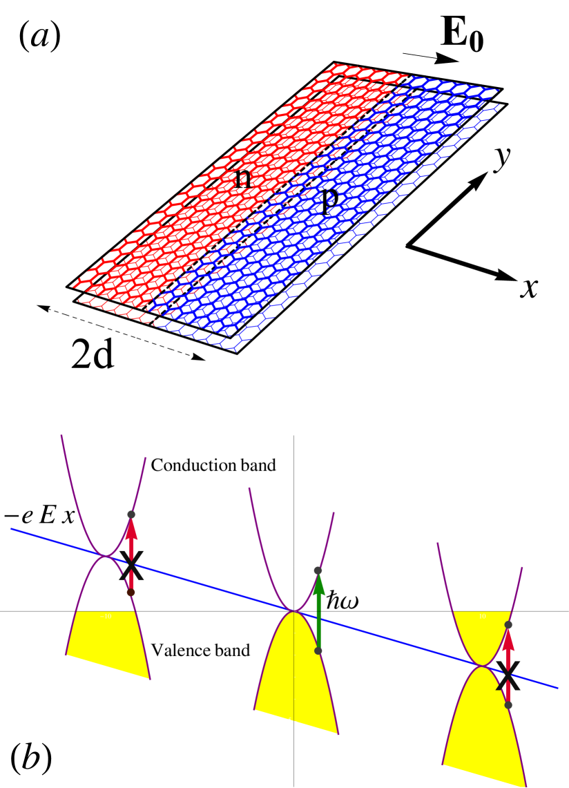
Figure 1: (Color online) (a) Bilayer graphene flake of width $2d$ is placed in electric field that separates p and n regions. Guided plasmons propagate along the $y$ axis and decay in the $x$ direction. (b) Schematic picture of the electron band structure: in equilibrium the sum of the electrostatic potential and kinetic energy of electrons (at the Fermi level) is constant. Vertical arrows indicate the possibility of optical absorption with a given frequency: while possible near the center of the flake (green non-crossed arrow), such transitions are forbidden (red crossed arrows) when both initial and final states are empty or occupied.

Under these conditions macroscopic hydrodynamic equations of the charged liquid can be applied. For the total electric field we have

$${\bf E}({\bf r},t)={\bf E}_{0}-\nabla\int d^{2}r^{\prime}\frac{\rho({\bf r^{\prime}},t)}{|{\bf r}-{\bf r^{\prime}}|}.$$ (2)

The fluctuating density $\rho({\bf r},t)$ obeys the charge conservation law

$$\dot{\rho}({\bf r},t)+\nabla\cdot{\bf J}({\bf r},t)=0.$$ (3)

While the two relations (2) and (3) are quite generic, the remaining equation for the electric current is system specific. For single-layer graphene it has been discussed in Refs. sachdev, and MSS, . The band structure of bilayer graphene consists of four bands that originate from the coupling of two Dirac cones of the two layers.cn The two outside bands are separated by a large band gap $\sim 0.6$ eV and will therefore be ignored here. The remaining two bands touch each other (in the absence of interlayer bias) and are parabolic, $\pm p^{2}/2m$, see Fig. 1, with the effective mass $m=0.05m_{0}$, where $m_{0}$ is the vacuum electron mass. For parabolic bands we find (see Appendix A for derivation)

$${\bf\dot{J}}=\frac{|\rho|}{m}\left(e{\bf E}-\nabla\mu\right);$$ (4)

here the chemical potential is related to the induced charge density via $\mu=-\pi\rho/2me$, where the fourfold (spin and valley) degeneracy is taken into account. The form of Eq. (4) is readily recognized from the usual ac Drude conductivity $\sigma={ie|\rho|}/{m\omega}$ if one notes that the expression in the brackets is simply the gradient of the electrochemical potential. The main difference comes from the fact that the effective “Drude conductivity” can depend on the coordinates (and time) via $|\rho|$.

II.1 Mean charge distribution

In equilibrium electric current is absent, ${\bf J}=0$, and the mean density of charges $\rho_{0}(x)$ obeys the equation

$${E_{0}x+2\int_{0}^{d}dx^{\prime}\rho_{0}(x^{\prime})\ln{\frac{x+x^{\prime}}{|x-x^{\prime}|}}+\frac{\pi a_{B}}{2}\rho_{0}(x)=0}.$$ (5)

This is the Thomas-Fermi equation where the first two terms describe electrostatics of an ideal metal strip. The last term takes into account that the screening radius is finite, the latter being of the same order as the Bohr radius $a_{B}={\hbar^{2}}/{me^{2}}\approx 10.6~{}\AA$. When the width of the flake is much greater than the Bohr radius, $d\gg a_{B}$, which is the case for any practical situation, the last term in Eq. (5) is negligible and the solution to the remaining integral equation is simply

$$\rho_{0}(x)=\frac{E_{0}x}{\sqrt{d^{2}-x^{2}}}.$$ (6)

This solution is known SMR from the method of conformal mapping for the two-dimensional Laplace equation, but it is most easily verified by a direct substitution into Eq. (5). Expression (6) is applicable everywhere except very close to an edge, where in principle the last term in Eq. (5) would provide regularization of the square-root singularity in the mean density. Such a procedure, however, strictly speaking, would exceed the accuracy of our semiclassical treatment. Indeed, as follows from Eq. (6), the last term in Eq. (5) becomes comparable with the first two at $d-x\sim a_{B}^{2}/d$, which is a length of the order of lattice spacing (or even smaller), where fully quantum-mechanical treatment is warranted. Fortunately for our purposes, the singularity in Eq. (6) is integrable and its presence will not affect the subsequent calculations.

II.2 Plasma oscillations

Plasmons are charge density oscillations propagating on top of the equilibrium profile , Eq. (6),

$$\rho=\rho_{0}(x)+\delta\rho({\bf r},t).$$ (7)

Equations (2)-(4) can be linearized with respect to the density variation $\delta\rho({\bf r},t)$. The latter will be taken in the form of a plane wave propagating along the junction, $\delta\rho({\bf r},t)=\chi(x)\exp(i\omega t-iqy)$. By substituting for electric field ${\bf E}$ and current ${\bf J}$ in Eq. (3) we obtain the following integrodifferential equation for the oscillating density profile,

$$\omega^{2}\chi(x)+\frac{2e}{m}\left[\frac{d}{dx}|\rho_{0}(x)|\frac{d}{dx}-q^{2}|\rho_{0}(x)|\right]$$

$$\times\int_{-d}^{d}dx^{\prime}\chi(x^{\prime})K_{0}(q|x-x^{\prime}|)=0,$$ (8)

where $K_{0}$ is the modified Bessel function of the second kind. Note that in deriving Eq. (II.2) we neglect the $\nabla\mu$ term in Eq. (4). As can be readily seen, its contribution is small by the parameter $a_{B}/\lambda\ll 1$.

Equation (II.2) is reminiscent of the equation for single-layer graphene,MSS where $\sqrt{|\rho_{0}(x)|}$ takes the place of $|\rho_{0}(x)|$. This difference makes the solution of the bilayer problem both simpler and trickier. In the most interesting case of a wide strip, $\lambda\ll d$, the confinement of plasmons originates from the gradient of the equilibrium charge density. Since, as we find below, plasmon oscillations extend over distances of the order of their wavelength in the transverse $x$ direction, the limits of integration in Eq. (II.2) can be extended to infinity while the mean density approximated with $\rho_{0}(x)=E_{0}x/d$. The plasmon momentum can then be conveniently scaled away with the substitution $qx=\xi$. Furthermore, using the equation for the modified Bessel function, $\tau K_{0}^{\prime\prime}(|\tau|)+K_{0}^{\prime}(|\tau|)=\tau K_{0}(|\tau|)$, it is convenient to rewrite the differential operation in Eq. (II.2) as follows: $(\frac{d}{d\xi}|\xi|\frac{d}{d\xi}-|\xi|)K_{0}(|\xi-\xi^{\prime}|)=\xi^{\prime}\text{sgn}~{}\xi(\frac{d^{2}}{d\xi^{2}}-1)K_{0}(|\xi-\xi^{\prime}|)$. Equation (II.2) then becomes ($\xi=qx$):

$$\omega^{2}\chi(\xi)+\frac{2eE}{md}\text{sgn}~{}\xi\biggl{(}\frac{d^{2}}{d\xi^{2}}-1\biggr{)}$$

$$\times\int_{-\infty}^{\infty}d\xi^{\prime}\xi^{\prime}\chi(\xi^{\prime})K_{0}(|\xi-\xi^{\prime}|)=0,$$ (9)

that in the Fourier representation acquires the form

$$\omega^{2}\chi(k)=-\frac{4\pi eE_{0}}{md}~{}{P}\int_{-\infty}^{\infty}\frac{dk^{\prime}}{2\pi}\,\frac{\sqrt{1+k^{\prime 2}}}{k^{\prime}-k}\frac{d\chi(k^{\prime})}{dk^{\prime}},$$ (10)

where $P$ stands for the principal value of integral. The integral equation (10) should determine the discrete spectrum of plasmon eigenvalues $\omega_{n}$. As expected, from the symmetry of the system, the solutions possess definite parity. It can be seen that Eq. (10) has even solutions

$$\chi^{(+)}_{\alpha}(k)=\cosh{\left(\frac{\pi\alpha}{2}\right)}\cos\Bigl{(}\alpha~{}\text{arcsinh}~{}{k}\Bigr{)},$$ (11)

and odd solutions

$$\chi^{(-)}_{\alpha}(k)=i\sinh{\left(\frac{\pi\alpha}{2}\right)}\sin\Bigl{(}\alpha~{}\text{arcsinh}~{}{k}\Bigr{)},$$ (12)

where $\alpha$ is an arbitrary positive number. This follows from the following relations

$${P}\int\limits_{-\infty}^{\infty}dt\frac{\cosh t\sin(\alpha t)}{\sinh t-\sinh\tau}=\frac{\pi\cos(\alpha\tau)}{\tanh(\pi\alpha/2)},$$ (13)

$${P}\int\limits_{-\infty}^{\infty}dt\frac{\cosh t\cos(\alpha t)}{\sinh t-\sinh\tau}=-\pi\tanh(\pi\alpha/2)\sin(\alpha\tau),\qquad$$ (14)

that can be proven by calculating the corresponding integrals with the help of adding an infinite semicircle in the complex plane and summing over the residues; see Appendix B. The corresponding spectrum of eigenvalues is gapped for the even modes,

$$\omega^{2}_{+}(\alpha)=\frac{2\pi eE_{0}}{md}\frac{\alpha}{\tanh(\pi\alpha/2)},$$ (15)

and gapless for the odd modes,

$$\omega^{2}_{-}(\alpha)=\frac{2\pi eE_{0}}{md}\alpha\tanh(\pi\alpha/2).$$ (16)

Finally, we note that the even and odd solutions obey a very simple relation in the real space,

$$\chi^{(-)}_{\alpha}(\xi)=\text{sgn}(\xi)\chi^{(+)}_{\alpha}(\xi).$$ (17)

This can be obtained by noticing that $\chi^{(+)}(k)$ and $\chi^{(-)}(k)$ are related by the Hilbert transform: the direct substitution of the solutions (11) and (12) into Eq. (10) yields

$$\chi^{(+)}_{\alpha}(k)=-i{P}\int_{-\infty}^{\infty}\frac{dk^{\prime}}{\pi}\frac{\chi^{(-)}_{\alpha}(k^{\prime})}{k^{\prime}-k},$$ (18)

which is the Fourier transform of Eq. (17).

The most surprising feature of the obtained solutions is the continuity of the spectrum of plasmon frequencies, which is in a seeming contradiction to the fact that plasmon modes are localized in the transverse direction. To elucidate the physical origin of this finding let us find the explicit form of our solutions in real space. Due to Eq. (17) it is sufficient to consider $\chi_{\alpha}^{(+)}(\xi)$ for positive arguments, $\xi>0$. As shown in Appendix B the solution is given by the modified Bessel function of the imaginary order,

$$\chi^{(+)}_{\alpha}(\xi)=\int\limits_{-\infty}^{\infty}\frac{dk}{2\pi}e^{ik\xi}\chi^{(+)}_{\alpha}(k)=\frac{\alpha\sinh(\pi\alpha)}{2\pi\xi}$$

$$\times\int\limits_{0}^{\infty}dte^{-\xi\cosh t}\cos(\alpha t)=\frac{\alpha\sinh(\pi\alpha)}{2\pi\xi}K_{i\alpha}(\xi).$$ (19)

For large distances, $\xi\gg 1$, the asymptotic behavior is exponential,

$$\chi^{(+)}_{\alpha}(\xi)\propto\frac{e^{-\xi}}{\xi^{3/2}}.$$ (20)

We indeed obtain that guided plasmons are localized on the distances of order of their wavelengths $\sim\lambda$.

The behavior at small distances, $\xi\ll 1$, is more peculiar:

$$\chi^{(+)}_{\alpha}(\xi)\approx-\frac{\alpha}{2\xi}\,\text{Im}~{}\frac{(\xi/2)^{i\alpha}}{\Gamma(1+i\alpha)}.$$ (21)

We observe that at small distances the solutions Eq. (II.2) have infinitely many nodes, which is formally responsible for the continuity of their spectrum. Noteworthy is the similarity between our charge density $\chi^{(+)}_{\alpha}$ and the wave function of a quantum-mechanical particle moving in the attractive potential $V(\xi)=-{\alpha^{2}}/{\xi^{2}}$ in two dimensions, the situation that leads to a particle falling on the attraction center.LLIII It is therefore obvious that oscillatory behavior at $\xi\to 0$ is an artifact of the semiclassical approximation. The latter fails at small distances comparable with the Fermi wavelength (which gets large closer to the p-n junction line). Thus such fast oscillations are unphysical and would not have appeared in the fully quantum-mechanical treatment of electrons in electric field. Fortunately, the oscillatory behavior is only logarithmic and can be easily regularized. This can be performed by noting that the solutions $\chi_{\alpha}^{+}(\xi)$ smoothed over these fast unphysical oscillations vanish at $\xi\to 0$. The vanishing is most easily seen from the density accumulated at small distances: using Eq. (21) we find

$$\int\limits_{0}^{\xi}d\xi^{\prime}\chi^{(+)}_{\alpha}(\xi^{\prime})=A\cos{[\alpha\ln{(\xi/2)}-\beta]},$$ (22)

where $\beta$ is the phase of the complex quantity $\Gamma(1+i\alpha)$. The accumulated charge therefore oscillates with constant amplitude $A$ around zero value. We therefore impose the regularization requirement that the smoothed solution should vanish at distances smaller than some $a$ (see below) where the semiclassical approach ceases to be valid. From Eq. (II.2) we obtain the equation

$$K_{i\alpha}(qa)=0,$$ (23)

which determines the set of discreet values of $\alpha$. Note that the choice of Eq. (23) is natural for both the even and odd modes as the replacement of the oscillatory function $K_{i\alpha}(\xi)$ with any smoothed nonzero value would have led to the nonintegrable singularity in Eq. (II.2) at $\xi=0$.

Equation (23) constitutes the quantization condition that together with Eqs. (11) and (12) determines the spectrum of guided plasmon modes for wavelengths shorter than the width of the flake. For $\alpha\ll 1$ we obtain in the logarithmic accuracy the following analytic approximation:

$$\alpha_{n}=\frac{\pi n}{\ln{\displaystyle\left(\frac{2e^{-\gamma}}{qa}\right)}},~{}~{}~{}n=1,2,3,\,.\,.\,.\,,$$ (24)

where $\gamma=0.58$ is the Euler’s constant. The first three eigenfunctions $\chi^{(+)}_{\alpha_{n}}(\xi)$, $n=1,\,2$, and $3$, are plotted in Fig. 2.

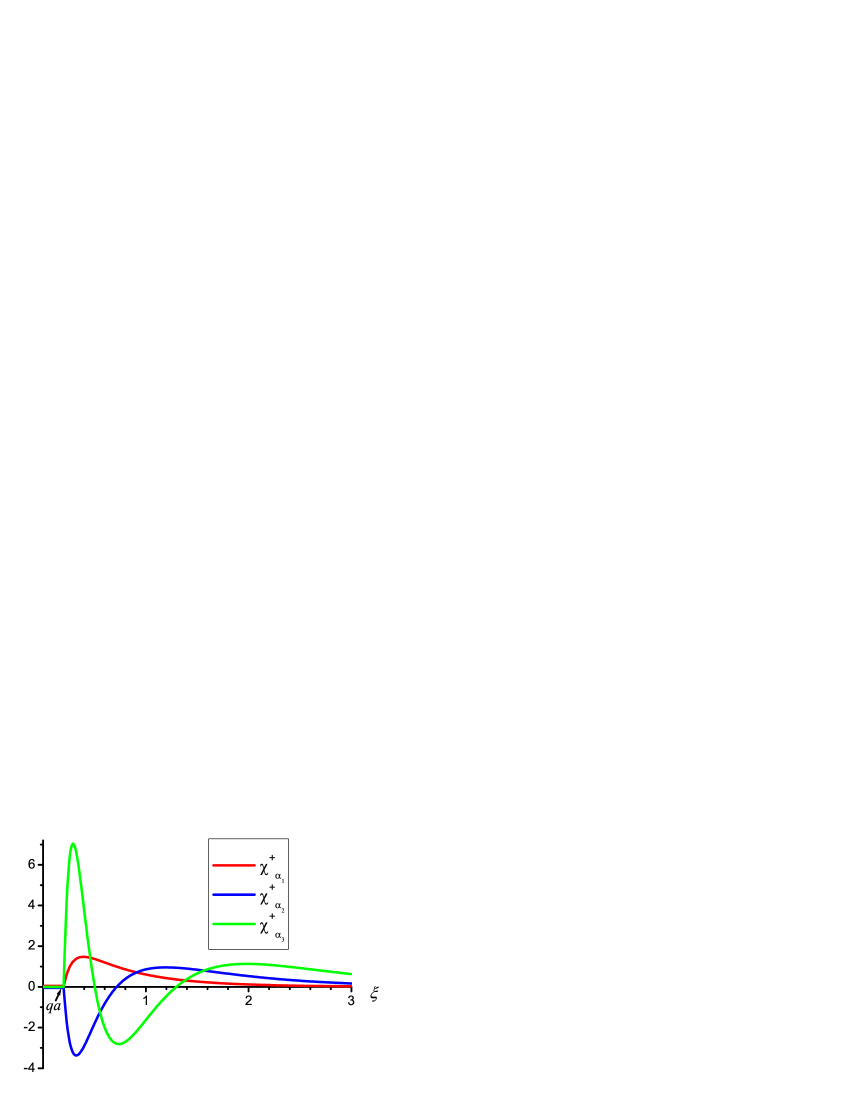
Figure 2: (Color online) The eigenfunctions $\chi^{(+)}_{\alpha_{n}}(\xi)$, Eq. (II.2), for three lowest values $n=1,\,2$, and $3$ and $qa=0.2$. The first mode (red) is node-less while the second one (blue) has just one node and the third (green) has two nodes and the sharpest peak. For the sake of convenience the functions $2\chi^{(+)}_{\alpha}(\xi)/\cosh{(\pi\alpha/2)}$ are plotted. The corresponding eigenvalues for $\alpha_{1}=1.44$, $\alpha_{2}=2.49$, $\alpha_{3}=3.42$ are found from Eq. (15).

The cutoff distance $a$ can be estimated as follows. The semiclassics fail at the distances of the order of the Fermi wavelength, $a\sim k_{F}^{-1}$. The latter, however, is a function of the coordinate, $k_{F}\sim(E_{0}x/de)^{1/2}$, cf. Eq. (6), and should be taken at the same distance, $x\sim a$. We therefore obtain that $a\sim l_{E}(d/l_{E})^{1/3}$, i.e., that the cutoff is mostly given by the electric length defined in Eq. (1) and exceeds the latter only by virtue of the factor $(d/l_{E})^{1/3}$.

II.3 Long wavelengths, $q\ll 1/d$

When the plasmon wavelength becomes comparable with $d$ (or exceeds it) the oscillating electric field extends beyond the width of the flake. The integral equation (II.2) has to be solved with the explicit boundary condition (unimportant previously) requiring that there is no particle flow across the edges of the system,

$$J_{x}(\pm d)=0.$$ (25)

In the limit $q\to 0$ the properties of plasmon spectrum can be elucidated without the exact solution. Eq. (II.2) becomes

$$\omega^{2}(0)\chi(\zeta)=-\frac{2eE_{0}}{md}\frac{d}{d\zeta}\frac{|\zeta|}{\sqrt{1-\zeta^{2}}}\int\limits_{-1}^{1}d\zeta^{\prime}\frac{\chi(\zeta^{\prime})}{\zeta^{\prime}-\zeta},$$ (26)

where $\zeta=x/d$. This equation has one zero eigenvalue, $\omega_{1}(0)=0$, which corresponds to the function

$$\chi(\zeta)=\frac{1}{\sqrt{1-\zeta^{2}}}.$$ (27)

The solution (27) simply describes charge distribution in the equipotentially charged metallic strip. For finite but small $q$ this mode develops into the usual one-dimensional plasmon with the spectrum (cf. Ref. MSS, for a similar discussion of the single-layer case)

$$\omega_{1+}^{2}(q)={\cal C}q^{2}\ln{(1/qd)}.$$ (28)

Here we denote by $\omega_{n\pm}$ the eigenfrequency of an even/odd mode with $n-1$ nodes across the half width of the flake $(0,d)$. In the short-wavelength limit it simply corresponds to $\omega_{\pm}(\alpha_{n})$; cf. Eqs. (15) and (16). The constant ${\cal C}$ is proportional to the total number of induced charges per unit length along the $y$ direction and can be most simply found by integrating the original Eq. (II.2) across the width of the graphene strip. Using the approximation $K_{0}(q|x-x^{\prime}|)=-\ln{q|x-x^{\prime}|}$ and noticing that the term containing the total derivative vanishes by virtue of the boundary condition (25), we obtain ${\cal C}=4eE_{0}d/m$. The logarithm in Eq. (28) originates from the long-range nature of Coulomb interaction.

Naively, one would expect the lowest-lying odd plasmon solution to be $(1-)$, i.e., to change its sign once, at the center of the flake, $\zeta=0$, but to keep the same sign across the half width of the sample. Remarkably, Eq. (26) does not admit an odd solution without at least one zero in the domain $(0,\,d)$, which also obeys the boundary condition Eq. (25). To see this, let us integrate Eq. (26) over $\zeta$ from $0$ to $1$. The boundary condition (25) implies that, as $\zeta\rightarrow 1$, we get

$$J_{x}(1)\propto\frac{\zeta}{\sqrt{1-\zeta^{2}}}\int\limits_{-1}^{1}d\zeta^{\prime}\frac{\chi(\zeta^{\prime})}{\zeta^{\prime}-\zeta}\Biggl{|}_{\zeta\to 1}=0.$$ (29)

Then we arrive at the relation

$$\frac{\omega^{2}(0)md}{2eE_{0}}\int\limits_{0}^{1}\!d\zeta\,\chi(\zeta)=\lim_{\zeta\rightarrow 0}\frac{|\zeta|}{\sqrt{1-\zeta^{2}}}\int\limits_{-1}^{1}d\zeta^{\prime}\frac{\chi(\zeta^{\prime})}{\zeta^{\prime}-\zeta}.$$ (30)

In physical terms this means that in order to have a net charge across the half width, $\int_{0}^{1}\!d\zeta\,\chi(\zeta)\neq 0$, there should be a nonvanishing current across the p-n junction, given by the right-hand side in Eq. (30). Nonvanishing of the limit in Eq. (30) implies in its turn that at the junction, $\zeta=0$, the induced electric field must be singularly strong,

$$E(\zeta\rightarrow 0)\propto\int\limits_{-1}^{1}d\zeta^{\prime}\frac{\chi(\zeta^{\prime})}{\zeta^{\prime}-\zeta}\sim\frac{1}{\zeta}.$$ (31)

To create such a strong field, the plasmon fluctuation should have a $\delta$-function singularity at $\zeta=0$, $\chi(\zeta)\propto\delta(\zeta)$. Such a situation is unphysical and in any case in conflict with the assumption that $\chi(\zeta)$ is an odd function. Thus we conclude that $\int_{0}^{1}d\xi\chi(\xi)=0$, and the lowest-lying odd plasmon eigenmode $(2-)$ should have at least three nodes across the width of the sample rather than a single node as might be intuitively expected.

The mode (28) is gapless because its electric potential is uniform across the flake. All other modes have nodes and therefore their frequencies do not tend to zero in the limit $q\to 0$ but instead have energy gaps $\omega_{n}(0)$ determined by Eq. (26). Without explicitly solving it we conclude from scaling that for all plasmons except the lowest even mode,

$$\omega^{2}_{n}(q\to 0)=\text{const}(n)\times\frac{eE_{0}}{md}.$$ (32)

In other words the plasmon spectrum at large wavelengths is determined by the same energy scale $eE_{0}/md$ as in the case of short wavelengths (15) and (16).

II.4 Mode order reversal at the intermediate wavelengths, $q\sim 1/d$.

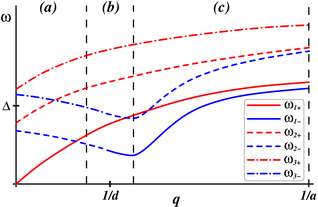
Figure 3: (Color online)The sketch of even plasmon (red monotonic curves) and odd plasmon (blue curves with minima around $1/d$) frequencies for $n=1$ (solid lines) and $n=2$ (dashed lines). The three regions, $q\ll 1/d$, $q\sim 1/d$, and $1/d\ll q<1/a$ are denoted by $(a)$, $(b)$, and $(c)$, respectively. With decreasing the wavelength through $\lambda\sim d$ the $n$th odd mode at $q\ll 1/d$ develops into the $n-1\,$th odd mode at $q\sim 1/d$, e.g., $(2-)$ becomes $(1-)$.

The results obtained so far have shown surprising reversal in the order of even and odd solutions. At long wavelengths, $\lambda\gg d$, shown as domain (a) in Fig. 3, the lowest energy mode is the gapless plasmon $\omega_{1}(q)$, Eq. (28). However, in the short-wavelength limit, $\lambda\ll d$, domain (c), the order is reversed as $\omega_{+}(\alpha_{n})>\omega_{-}(\alpha_{n})$, cf. Eqs. (15) and (16). Formally, as the short-wavelength cutoff is made smaller, $a\to 0$, the values of the lowest $\alpha_{n}$ decrease and the odd frequencies $\omega_{-}(\alpha_{n})$ approach zero; cf. Eq. (16). Such a change in the order of even and odd modes can be explained with simple physical picture of charge distribution illustrated in Fig. 4 for the first several modes. The lowest even mode’s charge distribution is nodeless across the width of the flake, and in the case of long wavelength $\lambda\gg d$, Fig. 4(a), produces a weak restoring longitudinal field $E\propto 1/\lambda^{2}$, resulting in the gapless spectrum (28). At shorter wavelengths the intermediate domain (b) $\lambda\sim d$, the distribution of charges for the lowest odd mode resembles a checkerboard with any plaquette of four charges composing a quadrupole. In the lowest even mode, on the other hand, the plaquette consists of two uncompensated dipoles that produce stronger electric field. We therefore conclude that around $\lambda\sim d$ the first odd plasmon becomes the lowest mode of the system.

For intermediate wavelengths $\lambda\sim d$, the mode $(1-)$ is no longer forbidden since $\int_{0}^{1}\!d\zeta\,\chi(\zeta)\neq 0$, as the charge transport occurs along the $y$ direction. The $(1-)$ mode evolves from the $(2-)$ mode at $q=0$ and at $\lambda\sim d$ has the frequency below that of the $(1+)$ plasmon. This reversal happens because the “checkerboard” pattern of the $(1-)$ mode significantly reduces the electric field compared with the $(1+)$ arrangement.

It appears that the reason for the change in the number of nodes in odd solutions is the linear decrease of the conductivity of a bilayer graphene near the line $x=0$ that prevents currents from flowing across that line so that the zero-node profile $(1-)$ can exist only when the wavelength becomes short enough, $\sim d$, for the longitudinal currents (along the $y$ axis) to be able to significantly affect the charge distribution. In contrast, in a monolayer graphene the conductivity vanishes only as the square root of $x$ and therefore currents across the junction can potentially remain finite if the fluctuating field has a $1/\sqrt{|x|}$ singularity, which is the case for odd solutions in a monolayer graphene.MSS

Let us emphasize that in plasmonic systems there is no inherent reason for even/odd modes to always have the same order. In particular, in 3D metal films the even mode has lower frequency,eco while in a system of two 2D electron layers separated by a dielectric the situation is reversed.dsm What makes guided plasmons in graphene bilayer peculiar is the crossover between these two cases for different wavelengths.

II.5 Comparison with the case of a monolayer, Ref. MSS,

It is useful to compare our findings for a bilayer graphene with the results of Ref. MSS, for a monolayer. In the latter case at short wavelengths $q\gg 1/d$ the solutions were doubly degenerate with a pair of even and odd modes having the same frequency. The frequencies were $\propto q^{1/4}$ while in the bilayer case they are [see Eqs. (15) and (16)] virtually independent of $q$ [up to the weak logarithmic dependence in Eq. (24)]. In addition, the dependence on the strength of the electric field creating the $p$-$n$ junction was $\propto E_{0}^{1/4}$ compared with the $E_{0}^{1/2}$ dependence for a bilayer.

The above-mentioned monolayer degeneracy was lifted in the long-wavelength limit $q\leq 1/d$ though not without some peculiarities. In particular, the order of the first four modes was $\omega_{1+}<\omega_{1-}<\omega_{2-}<\omega_{2+}$. In bilayer graphene the situation is more dramatic. From Eq. (16) we can see that, provided that $\ln{1/qa}\gg 1$, the frequencies of many odd modes decrease (soften) considerably with increasing the wavelength (decreasing $q$) in the region of intermediate wavelengths $q\sim 1/d$. However, that decrease in frequency does not persist at $q\to 0$ as the odd modes remain gapped there. The second unexpected finding is that the number of nodes in the odd modes increases by 1 with increasing the wavelength. This feature originates from the fast suppression of the conductivity of the bilayer near $x=0$ essentially decoupling electric currents in the $p$ and $n$ domains of the flake.

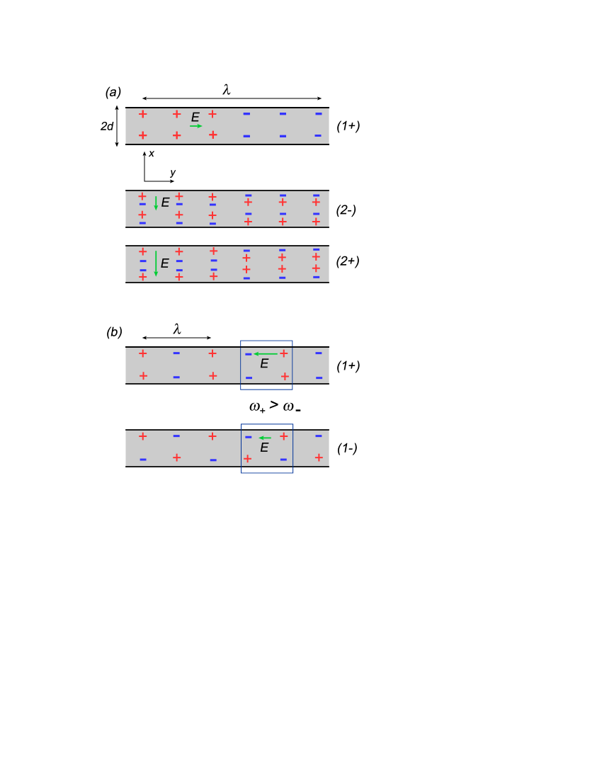
Figure 4: (Color online) Schematic charge distribution for the lowest plasmonic modes corresponding to different regions in Fig.  3. (a) For long wavelengths, $\lambda\gg d$, the lowest mode $(1+)$ is the quasi-one-dimensional plasmon with symmetric nodeless (across the flake) charge distribution and electric field pointed mostly along the $y$ direction. The magnitude of electric field vanishes with increasing the wavelength, in agreement with the gapless spectrum; Eq. (28). The second mode $(2-)$ is odd and gapped and has three nodes. A mode with a single node $(1-)$ is forbidden by the condition $\int_{0}^{d}\!dx\,\chi(x)=0$, valid for any gapped mode at $q\to 0$. The origin of that condition is the suppression of charge transport across the line separating $p$ and $n$ regions. The third mode $(2+)$ is even and has two nodes. The electric field in the modes $(2-)$ and $(2+)$ is mostly pointed along the $x$ direction. The field is stronger for the mode $(2+)$ (this fact could be easily inferred qualitatively from the picture of charge distribution), thus leading to $\omega_{2-}<\omega_{2+}$. (b) For intermediate wavelengths $\lambda\sim d$, the mode $(1-)$ is no longer forbidden and the $(1-)$ mode at $\lambda\sim d$ evolves from the $(2-)$ mode at $q=0$ and at $\lambda\sim d$ has the frequency below that of the $(1+)$ plasmon. This reversal happens because the checkerboard pattern of the $(1-)$ mode has lower electric field than the $(1+)$ mode.

III Experimental implications

The main obstacle in experimental observation of low-dimensional plasmons is that the latter are typically gapless. This makes it impossible to simply convert a photon into a plasmon with the conservation of both energy and momentum, so that more complicated experimental geometries are necessary.NB In the case considered in the present paper, plasmons confined near graphene bilayer p-n junctions are in general gapped, cf. Eqs. (15) and (32), and therefore straightforward absorption of long-wavelength (infrared) radiation is possible. Since the wavelength of the infrared radiation of interest to us reaches millimeter range the corresponding electric field is virtually homogeneous, so that only antisymmetric modes are likely to be excited. In contrast, symmetric modes have electric fields that are odd and therefore they do not couple to the radiation polarized along the $x$ axis. This can be seen in Fig. 4 where the electric field of the $(2+)$ mode along the $x$ axis in one half of the flake is the mirror reflection (along $x=0$) of the electric field in other half. In principle, symmetric modes could be excited by the longitudinal (along the $y$ axis) polarization. However, due to the conservation of momentum along the $y$ axis and small values of momentum of infrared photons, the phase space for such processes is rather restricted. Such absorption has characteristic frequencies $\Delta=\sqrt{4eE_{0}/md}$. Using the parameters of bilayer graphene we find

$$\Delta\approx 2.7~{}\text{eV}\times\frac{a_{B}}{l_{E}}\sqrt{\frac{a_{B}}{d}}.$$ (33)

For electric fields, $\sim 10^{6}$ V/m, the value of electric length is $l_{E}\sim 40$nm. Assuming $d\approx 1\mu$m for the size of the sample we obtain from Eq. (33) that $\Delta\sim 2$ meV. We therefore expect a threshold signature in the absorption spectrum of infrared radiation at these frequencies, which are very sensitive to the magnitude of the electric field creating the p-n junction.

We emphasize that the plasmon absorption happens in addition to the intersubband electron-hole absorption. The latter, however, is a smooth function of frequency. Indeed, interband absorption of a photon with frequency $\omega$ is possible only as long as the chemical potential (the distance to the Fermi level from the band degeneracy point $p=0$) does not exceed $\hbar\omega/2$; see Fig. 1(b). The former, expressed via the charge density, Eq. (6), is simply $\pi|\rho|/2me=\pi E_{0}|x|/2me\sqrt{d^{2}-x^{2}}$. Thus the corresponding transitions are allowed within a strip of $|x|<d/\sqrt{1+(\pi E_{0}/me\omega)^{2}}$. The intensity of the absorption is independent of frequency and simply determined by the intersubband ac (“minimal”) conductivity MC of bilayer, $e^{2}/2\hbar$. The frequency dependence of single-particle absorption is therefore simply determined by the width of the absorbing region,

$$A_{e-h}(\omega)\propto\frac{\omega d}{\sqrt{\pi^{2}E^{2}_{0}+m^{2}e^{2}\omega^{2}}}.$$ (34)

This expression describes a smooth background that exists in addition to the usual intrasubband Drude absorption. Its characteristic frequency $\hbar^{2}/ml_{E}^{2}$ depends linearly on the applied electric field and should be easily distinguishable by varying the electric field from the plasmon contribution whose frequency (33) is proportional to $E^{1/2}_{0}$.

IV Gated bilayer

The advantages of bilayer graphene for applications lie in the possibility of inducing a bandgap with the interlayer bias, studied both theoreticallyEMC ; LAF ; GLS ; FMC and experimentally.KCM ; ZTG ; MLS Since this is typically performed via the nearby metallic gates, we now discuss how the properties of guided plasmons are modified by the presence of such a gate, which is assumed to be positioned a distance $D$ from the bilayer. In addition, the presence of a bandgap leads to the appearance of a neutral strip of width $2h$; see Fig. 5. In this section after explaining how the general equations are changed, we consider three cases: (i) short wavelengths, $q^{-1}\ll D$, (ii) intermediate wavelengths, $D\ll q^{-1}\ll h$, and (iii) long wavelengths, $h\ll q^{-1}\ll d$.

Two modifications have to be made to our hydrodynamic equations. In particular, the induced electric field includes the additional contribution from image charges,

$${\bf E}({\bf r},t) = {\bf E}_{0}-\nabla\int d^{2}r^{\prime}\rho({\bf r^{\prime}},t)$$ (35)

$$\times\left(\frac{1}{|{\bf r}-{\bf r^{\prime}}|}-\frac{1}{\sqrt{({\bf r}-{\bf r^{\prime}})^{2}+4D^{2}}}\right).$$

The second modification should incorporate the presence of a gap $2U$ in the energy spectrum, $\epsilon(p)=\pm\sqrt{U^{2}+(p^{2}/2m)^{2}}$. The relation between the local chemical potential and the induced charge density now becomes

$$\mu=-\text{sgn}~{}(\rho)~{}\sqrt{U^{2}+\left(\frac{\pi\rho}{2me}\right)^{2}}.$$ (36)

The existence of a gap in the spectrum means that separation of electrons and holes is possible only when the applied in-plane electric field exceeds some value, $E_{0}\geq U/ed$. Even above this threshold p and n regions are separated by a neutral strip of width $2h=2U/eE$, as shown in Fig. 2. The mean distribution of the induced charges $\rho_{0}(x)$ is determined by the Thomas-Fermi equation

$$E_{0}x + \text{sgn}(x)\sqrt{\frac{U^{2}}{e^{2}}+\frac{\pi^{2}a_{B}^{2}}{4}\rho_{0}^{2}(x)}$$ (37)

$$+2\int_{0}^{d}dx^{\prime}\rho_{0}(x^{\prime})\ln{\frac{x+x^{\prime}}{|x-x^{\prime}|}}=0.$$

The second term under the square root can (similarly to Sec. II) be neglected everywhere except very close to the flake’s edges [more precisely, as long as $a_{B}\rho_{0}(x)$ is less than either $E_{0}x$ or $U/e$]. The resulting linear equation has been solved in Ref. SMR, in relation to the polarization of a nanotube array in the external electric field, yielding

$$\rho_{0}(x)=\text{sgn}(x)~{}E_{0}\sqrt{\frac{x^{2}-h^{2}}{d^{2}-x^{2}}}\>\Theta(|x|-h),$$ (38)

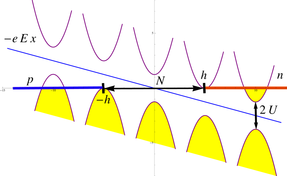
Figure 5: (Color online) Electron band structure across the bilayer with the energy gap of $2U$. The p (blue line starting from the point where the second lower peak on the left side touches the Fermi level and ending at the left end of the flake) and n regions (red line on the right side of the axis) are separated by a neutral (N) strip (black double-headed arrow) of width $2h=2U/eE$ determined by the energy gap and the slope of the scalar potential.

The equation of motion for plasmon oscillations is also modified by the gap in the spectrum, as explained in Appendix A; see Eq. (54). Solution of the corresponding general equation for the oscillating density is beyond the scope of the present paper. However, great simplification occurs if the gap is not very small, so that the width of the neutral strip is much greater than the Bohr radius, $h\gg a_{B}$. In this case the second term in the denominator of Eq. (54) is negligible compared with $U$, which amounts to the substitution

$$|\rho_{0}|\to\frac{\pi\rho_{0}^{2}}{2meU}$$ (39)

in Eq. (II.2). The second change to Eq. (II.2) comes from taking into account the image charges from Eq. (35). This is done by replacing $K_{0}(q|x-x^{\prime}|)$ with

$$K_{0}(q|x-x^{\prime}|)-K_{0}[q\sqrt{(x-x^{\prime})^{2}+4D^{2}}]$$

$$=\frac{1}{2}\int\limits_{-\infty}^{\infty}\frac{dk}{\sqrt{q^{2}+k^{2}}}\left(1-e^{-2D\sqrt{q^{2}+k^{2}}}\right)e^{ik(x-x^{\prime})}.$$ (40)

Below we elucidate plasmon dispersion for the case of a wide flake and a gate situated in close proximity to it, $D\ll h\ll d$.

(i) Short wavelengths, $q^{-1}\ll D$. In this case the effect of the image charges is negligible. Plasmons propagate along a boundary between a charged (p or n) domain and a neutral strip (N) and decay over a distance short compared to $h$. Thus modes localized near the p-N boundary are exponentially weakly coupled to n-N modes. The corresponding plasmon frequencies,

$$\omega^{2}\sim\frac{E_{0}^{2}h}{m^{2}d^{2}U},$$ (41)

are therefore doubly degenerate and independent of the wavelength.

(ii) Intermediate wavelengths, $D\ll q^{-1}\ll h$. The wavelength is still short enough to ensure that plasmons propagating near the two edges of the neutral strip do not “talk,” but the Coulomb interaction is screened by the gate. The expression in Eq. (IV) can be approximated with $2\pi D\delta(x-x^{\prime})$. Since only small $\tilde{x}=x-h\ll h$ are of interest, the density in Eqs. (37) and (39) can be approximated with ($\tilde{x}>0$)

$$\rho_{0}^{2}(\tilde{x})=\frac{2hE_{0}^{2}}{d^{2}}\tilde{x}$$ (42)

By virtue of the $\delta$ function the equation for the oscillating charge density becomes a differential one,

$$\frac{1}{\tilde{x}}\frac{d}{d\tilde{x}}\left(\tilde{x}\frac{d\chi(\tilde{x})}{d\tilde{x}}\right)+\left(\frac{\omega^{2}}{C^{2}\tilde{x}}-q^{2}\right)\chi(\tilde{x})=0,$$ (43)

where $C^{2}=\frac{4\pi^{2}E_{0}^{2}hD}{d^{2}m^{2}U}$. This equation is identical to that of a two-dimensional “hydrogen atom” with $-q^{2}$ playing the role of the energy and $\omega^{2}/C^{2}$ the role of the interaction constant. The corresponding quantization condition is simply $q=\omega^{2}/2C^{2}(n+1/2)$, which yields the spectrum

$$\omega^{2}_{n}=(n+1/2)\frac{8\pi^{2}\,E_{0}^{2}h\,D}{d^{2}m^{2}U}q,~{}~{}~{}n=0,1,2,\,.\,.\,.\,.$$ (44)

The corresponding eigenfunctions are given by the confluent hypergeometric function of the first kind,

$$\chi_{n}(\tilde{x})=e^{-q\tilde{x}}~{}_{1}F_{1}(-n,1,2q\tilde{x}).$$ (45)

Remarkably, the solutions (45) do not vanish at $\tilde{x}=x-h=0$. This indicates that the shape of the boundary of the neutral strip, created by “soft” electrostatic confinement, does not remain linear and itself fluctuates due to plasmon excitations.

(iii) For yet longer wavelengths, $h\ll q^{-1}\ll d$, the presence of the neutral strip is irrelevant as the field of plasmons extends over much larger distances. Assuming that the wavelength is still much smaller than the width $d$, we can use $\rho^{2}=E_{0}^{2}x^{2}/d^{2}$, cf.  Eq. (6). The $\delta$ function approximation from the previous paragraph still holds, yielding

$$\frac{1}{\xi^{2}}\frac{d}{d\xi}\left(\xi^{2}\frac{d\chi}{d\xi}\right)+\left(\frac{\omega^{2}}{C^{2}_{1}\xi^{2}}-1\right)\chi=0,$$ (46)

where $\xi=qx$, and $C_{1}^{2}=\frac{2\pi^{2}E_{0}^{2}D}{m^{2}d^{2}U}$. With the help of the substitution, $\chi(\xi)=f(\xi)/|\xi|$, Eq. (46) is reduced to

$$\frac{d^{2}f}{d\xi^{2}}+\left(\frac{\omega^{2}}{C^{2}_{1}\xi^{2}}-1\right)f=0,$$ (47)

which is the one-dimensional Schrödinger equation for the potential $\propto-1/\xi^{2}$. The singularity at $\xi=0$ needs to be regularized by cutting off at $\xi\approx qa$. Using the Bohr-Sommerfeld condition,

$$4\int\limits_{qa}^{\omega/C_{1}}d\xi\sqrt{\frac{\omega^{2}}{C_{1}^{2}\xi^{2}}-1}=2\pi\left(n+\frac{1}{2}\right),$$ (48)

we find the spectrum to be

$$\omega^{2}=\frac{\pi^{4}E_{0}^{2}D}{2m^{2}d^{2}U\ln^{2}(qa)}(n+1/2)^{2},~{}~{}~{}n=0,1,2,\,.\,.\,.\,.$$ (49)

The result (49) becomes more accurate for $n\gg 1$, since the WKB applicability condition for Eq. (47) requires that $\omega\gg C_{1}$. Still, even for $n\sim 1$ the expression (49) captures the correct dependence on the gap $U$ and the strength of the external field $E_{0}$.

To conclude the discussion of the gated bilayer, let us note that only in the intermediate case (ii) does the plasmon frequency demonstrate dependence on the wave number, namely when the wavelength is long enough to ensure screening by image charges, but still sufficiently short compared with the width of the neutral strip. In all three regimes the dependence of plasmon spectra on electric field $E_{0}$ is linear in contrast to a gapless case, where the corresponding dependence is square root; see Eqs. (15), (16), and (32).

V Summary

Bilayer graphene is a gapless (or weakly gapped) system that is charge neutral when undoped. Separation of charges, however, occurs with even weak external electric fields applied along the plane of bilayer; see Fig. 1. The induced charge density Eq. (6) follows from the solution of the electrostatic problem. The gradient of charge density near the p-n junction line $x=0$ leads to the confinement of charge oscillations (plasmons) resulting in their one-dimensional propagation along the junction. Physically, confinement in the transverse direction can be understood as follows. Since plasmon “stiffness” increases with increasing the local charge density, plasmons of lower frequency tend to be located closer to the p-n junction and to decay into the region of higher density.

Within a continuous hydrodynamic approach for charge-density oscillations the plasmon modes are determined from the integrodifferential eigenvalue problem, Eq. (10). The latter allows for exact solutions, Eqs. (11) and (12), with the discretization of the spectrum being a consequence of the regularization of the logarithmic singularity, Eq. (23). For small wave vectors $q$ the lowest mode is an even solution that is a conventional 1D plasmon with logarithmic velocity. At $q\sim 1/d$ the order is reversed and the first odd solution becomes the mode with the lowest energy.

From the practical standpoint guided plasmon modes could potentially be used for “plasmon transistors.”HAA The immediate experimental signatures of the guided plasmons, however, can be most directly measured in the optical absorption. While the electron-hole intersubband excitations lead to a smooth continuum, Eq. (34), the gapped plasmon spectrum of antisymmetric modes should result in a threshold behavior at a frequency $\sim eE_{0}/md$ sensitive to the applied electric field.

Appendix A Hydrodynamic equations

Equations (3) and (4) can be derived from the Boltzmann equation for the electron distribution function $f_{\bf p}$,

$$\frac{\partial f_{\bf p}}{\partial t}+{\bf v}\cdot\nabla f_{\bf p}+e{\bf E}\cdot\frac{\partial f_{\bf p}}{\partial\bf p}=I[f_{\bf p}],$$ (50)

where the right-hand side is the collision integral.LLX Since the latter conserves the number of electrons, integrating the equation over the entire momentum space yields the continuity equation (3). Hydrodynamic approximation is applicable when a distribution function deviates only slightly from a local equilibrium distribution with the chemical potential $\mu({\bf r},t)$ (which is equivalent to specifying the local density $\rho$). The deviation is due to the drift of particles with the average velocity being considerably smaller than the Fermi velocity $v_{F}$, and characterized by a local current density ${\bf J}({\bf r},t)$:

$$f_{\bf p}({\bf r},t)=\Theta(\mu({\bf r},t)-\epsilon_{p})+2\frac{{\bf v}\cdot{\bf J}({\bf r},t)}{ev_{F}^{2}\nu(\mu)}\delta[\mu({\bf r},t)-\epsilon_{p}],$$ (51)

where $\nu(\mu)$ is the density of states at the Fermi level. Such an ansatz is nothing but the expansion over angular harmonics truncated after the first term. Multiplying Eq. (50) by $e{\bf v}$ and performing the same operation, we can obtain the equation for electric current,

$$\frac{\partial\bf J}{\partial t}+e\sum_{\bf p}{\bf v}({\bf v}\cdot\nabla f_{\bf p})+e^{2}\sum_{\bf p}{\bf v}\biggl{(}{\bf E}\cdot\frac{\partial f_{\bf p}}{\partial\bf p}\biggr{)}$$

$$=e\sum_{\bf p}{\bf v}I[f_{\bf p}].$$ (52)

The last term represents collision relaxation of the electric current and for small currents (linear response) may be written as $-{\bf J}/\tau$, where $\tau$ is the transport mean free time. Substituting Eq. (51) into Eq. (A) we get

$$\frac{\partial\bf J}{\partial t}+\frac{{\bf J}}{\tau}=\frac{1}{2}ev_{F}^{2}\nu(\mu)(e{\bf E}-\nabla\mu).$$ (53)

This expression generalizes the usual Drude conductivity onto the case of coordinate- and time-dependent density of 2D electron gas. For frequencies exceeding the collision rate the second term in the left-hand side can be neglected. If the gap is present the spectrum is $\epsilon(p)=\sqrt{U^{2}+(p^{2}/2m)^{2}}$. Calculating the Fermi velocity $v_{F}=d\mu/dp_{F}$ and the density of states, $\nu(\mu)=2p_{F}/\pi v_{F}$, we obtain

$$\dot{\bf J}=\frac{\pi}{2m^{2}e}\frac{\rho^{2}}{\sqrt{U^{2}+\left(\frac{\pi\rho}{2me}\right)^{2}}}(e{\bf E}-\nabla\mu).$$ (54)

In the case where there is no gap, $U=0$, Eq. (4) is recovered.

Appendix B Integral relations

Integral relations, Eqs. (13) and (14), can be established by considering the integral

$${P}\!\!\int\limits_{-\infty}^{\infty}\!dt\,\frac{\cosh t\,e^{i\alpha t}}{\sinh t-\sinh\tau}.$$ (55)

This integral can be evaluated by noticing that in the upper plane of the complex variable $t$, the integrand is exponentially suppressed on the infinite semicircle, $t=Re^{i\varphi}$, $0\leq\varphi\leq\pi$, $R\rightarrow\infty$; see Fig. 6(a). Then the integral equals the sum of residues at $t=\tau+2\pi ni$ and $t=-\tau+\pi(2n-1)i$, where $n=1,2,\,.\,.\,.$, times $2\pi i$, plus the residue at $t=\tau$ times $\pi i$, which is due to the principal integration. After the integral of Eq. (55) is evaluated, Eqs. (13) and (14) hold as being the real and imaginary parts of it, respectively.

Upon replacing $k\mapsto\sinh\tau$ and $k^{\prime}\mapsto\sinh t$, the integrodifferential equation (10) acquires the form

$$\omega^{2}\tilde{\chi}(\tau)=-\frac{4\pi eE}{md}~{}{P}\!\!\int\limits_{-\infty}^{\infty}\!\frac{dt}{2\pi}\,\frac{\cosh t}{\sinh t-\sinh\tau}\frac{d\tilde{\chi}(t)}{dt},$$ (56)

where $\tilde{\chi}(t)=\chi(\sinh t)$. Equations (13) and (14) imply that $\tilde{\chi}(t)=\cos(\alpha t)$ and $\tilde{\chi}(t)=\sin(\alpha t)$ solve the integrodifferential equation, Eq. (56), yielding the spectra Eqs. (15) and (16), respectively. Going back to the original variable, $t=\text{arcsinh}\,k$, we recover the even and odd solutions, Eqs. (11) and (12), which in addition are multiplied by factors $\cosh(\pi\alpha/2)$ and $i\sinh(\pi\alpha/2)$, respectively, for the sake of further convenience. This can be done without destroying the solutions as these factors are constants with respect to the variable $k$.

Figure 6: (a) Contour in the complex plane for the calculation of the integral (55); the singularities in the integrand are indicated by the dots; (b) deformation of the contour from the real axis for the calculation of the integral (58).

In the remaining portion of this Appendix we establish the relation Eq. (II.2). Consider the Fourier transform

$$\chi^{(+)}_{\alpha}(\xi)=\int\limits_{-\infty}^{\infty}\frac{dk}{2\pi}\,e^{ik\xi}\chi^{(+)}_{\alpha}(k).$$ (57)

After performing a change, $k=\sinh t$, and integrating by parts, we rewrite Eq. (57) in the form

$$\chi^{(+)}_{\alpha}(\xi)=\frac{\alpha\cosh(\pi\alpha/2)}{2\pi i\xi}\int\limits_{-\infty}^{\infty}\!dt\,e^{i\xi\sinh t}\sin(\alpha t).$$ (58)

The integrand in Eq. (58) is a holomorphic function of the complex variable $t$, so that the integration contour can be deformed from real axis to the horizontal line, $-\infty+i\pi/2\leq t\leq\infty+i\pi/2$; see Fig. 6(b). In doing this we also notice that the integrals over the vertical parts, $-\infty\leq t\leq-\infty+i\pi/2$ and $\infty+i\pi/2\leq t\leq\infty$, are suppressed. Then Eq. (58) turns into the relation

$$\chi^{(+)}_{\alpha}(\xi)= \!\!\!\!\!\frac{\alpha\cosh(\pi\alpha/2)}{2\pi i\xi}\!\!\int\limits_{-\infty}^{\infty}\!\!dt\,e^{-\xi\cosh t}\bigl{[}\sin(\alpha t)\cosh(\pi\alpha/2)$$ (59)

$$+i\cos(\alpha t)\sinh(\pi\alpha/2)\bigr{]}.$$

The first term in the rectangular brackets turns to zero as being an odd function of $t$, and we finally arrive at the integral representation,

$$\chi^{(+)}_{\alpha}(\xi)=\frac{\alpha\sinh(\pi\alpha)}{2\pi\xi}\int\limits_{0}^{\infty}\!dt\,e^{-\xi\cosh t}\cos(\alpha t).$$ (60)

References

- (1) M. Wilson, Phys. Today 59(10), No. 1, 21 (2006).
- (2) A. K. Geim and K.S. Novoselov, Nature Mater. 6, 183 (2007).
- (3) H. A. Atwater, Sci. Am. 296(4), 56 63 (2007).
- (4) S. A. Maier, Plasmonics: Fundamentals and Applications (Springer, New York, 2007).
- (5) O. Vafek, Phys. Rev. Lett. 97, 266406 (2006).
- (6) E.H. Hwang and S. Das Sarma, Phys. Rev. B 75, 205418 (2007).
- (7) F. Stern, Phys. Rev. Lett. 18, 546 (1967).
- (8) E. G. Mishchenko, A. V. Shytov, and P. G. Silvestrov, Phys. Rev. Lett. 104, 156806 (2010).
- (9) A. H. Castro Neto, F. Guinea, N. M. R. Peres, K. S. Novoselov, and A. K. Geim, Rev. Mod. Phys. 81, 109 (2009).
- (10) E. McCann and V. I. Falko, Phys. Rev. Lett. 96, 086805 (2006).
- (11) X. F. Wang and T. Chakraborty, Phys. Rev. B 81, 081402(R) (2010).
- (12) R. Sensarma, E. H. Hwang, S. Das Sarma, Phys. Rev. B 82, 195428 (2010).
- (13) M. Jablan, H. Buljan, and M. Soljacic, Optics Express, 19, 11236 (2011).
- (14) O. V. Gamayun, arXiv:1103.4597.
- (15) L. Jing, J. Velasco, Ph. Kratz, G. Liu, W. Bao, M. Bockrath, Ch. N. Lau, Nano Lett. 10, 4000 (2010).
- (16) C. J. Poole, Solid State Commun. 150, 632 (2010).
- (17) R. Nandkishore and L. Levitov, arXiv:1101.0436.
- (18) S. Park, H.-S. Sim, arXiv:1103.3331.
- (19) M. Mueller, L. Fritz, S. Sachdev, and J. Schmalian, in “Advances in theoretical physics: Landau Memorial Conference”,edited by Vladimir Lebedev and Mikhail Feigel’man, AIP Conf. Proc. No. 1134 (AIP, Melville, NY, 2009), p. 170.
- (20) T. A. Sedrakyan, E. G. Mishchenko, and M. E. Raikh, Phys. Rev. B 74, 235423 (2006).
- (21) L. D. Landau and E. M. Lifshitz, Quantum Mechanics: Non-Relativistic Theory, (Addison-Wesley, Reading, Mass., Oxford, 1958).
- (22) E. N. Economou, Phys. Rev. 182, 539 (1969).
- (23) S. Das Sarma and A. Madhukar, Phys. Rev. B 23, 805 (1981).
- (24) L. Novotny and B. Hecht, Principles of Nano-Optics, (Cambridge University Press, New York, 2006).
- (25) K. S. Novoselov, E. McCann, S. V. Morozov, V. I. Falko, M. I. Katsnelson, U. Zeitler, D. Jiang, F. Schedin, and A. K. Geim, Nature Phys. 2, 177 (2006); M. I. Katsnelson, Eur. Phys. J. B 52, 151 (2006).
- (26) E. McCann, Phys. Rev. B 74, 161403(R) (2006).
- (27) L. A. Falkovsky, Phys. Rev. B 80, 113413 (2009).
- (28) P. Gava, M. Lazzeri, A. M. Saitta, F. Mauri, Phys. Rev. B 79, 165431 (2009).
- (29) M. M. Fogler, E. McCann, Phys. Rev. B 82, 197401 (2010).
- (30) A. B. Kuzmenko, I. Crassee, D. van der Marel, P. Blake, and K. S. Novoselov, Phys. Rev. B 80, 165406 (2009).
- (31) Y. Zhang, T.-T. Tang, C. Girit, Z. Hao, M. C. Martin, A. Zettl, M.F. Crommie, Y. R. Shen, and F. Wang, Nature 459, 820 (2009).
- (32) K. F. Mak, C. H. Lui, J. Shan, and T. F. Heinz, Phys. Rev. Lett. 102, 256405 (2009).
- (33) E. M. Lifshitz and L. P. Pitaevskii, Physical Kinetics, (Butterworth-Heinenann, Oxford, 1999).