Simulation-based optimal Bayesian experimental design for nonlinear systems

Abstract

The optimal selection of experimental conditions is essential to maximizing the value of data for inference and prediction, particularly in situations where experiments are time-consuming and expensive to conduct. We propose a general mathematical framework and an algorithmic approach for optimal experimental design with nonlinear simulation-based models; in particular, we focus on finding sets of experiments that provide the most information about targeted sets of parameters.

Our framework employs a Bayesian statistical setting, which provides a foundation for inference from noisy, indirect, and incomplete data, and a natural mechanism for incorporating heterogeneous sources of information. An objective function is constructed from information theoretic measures, reflecting expected information gain from proposed combinations of experiments. Polynomial chaos approximations and a two-stage Monte Carlo sampling method are used to evaluate the expected information gain. Stochastic approximation algorithms are then used to make optimization feasible in computationally intensive and high-dimensional settings. These algorithms are demonstrated on model problems and on nonlinear parameter inference problems arising in detailed combustion kinetics.

1 Introduction

Experimental data play an essential role in developing and refining models of physical systems. For example, data may be used to update knowledge of parameters in a model or to discriminate among competing models. Whether obtained through field observations or laboratory experiments, however, data may be difficult and expensive to acquire. Even controlled experiments can be time-consuming or delicate to perform. In this context, maximizing the value of experimental data—designing experiments to be “optimal” by some appropriate measure—can dramatically accelerate the modeling process. Experimental design thus encompasses questions of where and when to measure, which variables to interrogate, and what experimental conditions to employ.

These questions have received much attention in the statistics community and in many science and engineering applications. When observables depend linearly on parameters of interest, common solution criteria for the optimal experimental design problem are written as functionals of the information matrix [1]. These criteria include the well-known ‘alphabetic optimality’ conditions, e.g., $A$-optimality to minimize the average variance of parameter estimates, or $G$-optimality to minimize the maximum variance of model predictions. Bayesian analogues of alphabetic optimality, reflecting prior and posterior uncertainty in the model parameters, can be derived from a decision-theoretic point of view [2]. For instance, Bayesian $D$-optimality can be obtained from a utility function containing Shannon information while Bayesian $A$-optimality may be derived from a squared error loss. In the case of linear-Gaussian models, the criteria of Bayesian alphabetic optimality reduce to mathematical forms that parallel their non-Bayesian counterparts [2].

For nonlinear models, however, exact evaluation of optimal design criteria is much more challenging. More tractable design criteria can be obtained by imposing additional assumptions, effectively changing the form of the objective; these assumptions include linearizations of the forward model, Gaussian approximations of the posterior distribution, and additional assumptions on the marginal distribution of the data [2]. In the Bayesian setting, such assumptions lead to design criteria that may be understood as approximations of an expected utility. Most of these involve prior expectations of the Fisher information matrix [3]. Cruder “locally optimal” approximations require selecting a “best guess” value of the unknown model parameters and maximizing some functional of the Fisher information evaluated at this point [4]. None of these approximations, though, is suitable when the parameter distribution is broad or when it departs significantly from normality [5]. A more general design framework, free of these limiting assumptions, is preferred [6, 7].

More rigorous information theoretic criteria have been proposed throughout the literature. The seminal paper of Lindley [8] suggests using expected gain in Shannon information, from prior to posterior, as a measure of the information provided by an experiment; the same objective can be justified from a decision theoretic perspective [9, 10]. Sebastiani and Wynn [11] propose selecting experiments for which the marginal distribution of the data has maximum Shannon entropy; this may be understood as a special case of Lindley’s criterion. Maximum entropy sampling (MES) has seen use in applications ranging from astronomy [12] to geophysics [13], and is well suited to nonlinear models. Reverting to Lindley’s criterion, Ryan [14] introduces a Monte Carlo estimator of expected information gain to design experiments for a model of material fatigue. Terejanu et al. [15] use a kernel estimator of mutual information (equivalent to expected information gain) to identify parameters in chemical kinetic model. The latter two studies evaluate their criteria on every element of a finite set of possible designs (on the order of ten designs in these examples), and thus sidestep the challenge of optimizing the design criterion over general design spaces. And both report significant limitations due to computation expense; [14] concludes that “full blown search” over the design space is infeasible, and that two order-of-magnitude gains in computational efficiency would be required even to discriminate among the enumerated designs.

The application of optimization methods to experimental design has thus favored simpler design objectives. The chemical engineering community, for example, has tended to use linearized and locally optimal [16] design criteria or other objectives [17] for which deterministic optimization strategies are suitable. But in the broader context of decision theoretic design formulations, sampling is required. [18] proposes a curve fitting scheme wherein the expected utility was fit with a regression model, using Monte Carlo samples over the design space. This scheme relies on problem-specific intuition about the character of the expected utility surface. Clyde et al. [19] explore the joint design, parameter, and data space with a Markov chain Monte Carlo (MCMC) sampler; this strategy combines integration with optimization, such that the marginal distribution of sampled designs is proportional to the expected utility. This idea is extended with simulated annealing in [20] to achieve more efficient maximization of the expected utility. [19, 20] use expected utilities as design criteria but do not pursue information theoretic design metrics. Indeed, direct optimization of information theoretic metrics has seen much less development. Building on the enumeration approaches of [13, 14, 15] and the one-dimensional design space considered in [12], [7] iteratively finds MES designs in multi-dimensional spaces by greedily choosing one component of the design vector at a time. Hamada et al. [21] also find “near-optimal” designs for linear and nonlinear regression problems by maximizing expected information gain via genetic algorithms. But the coupling of rigorous information theoretic design criteria, complex physics-based models, and efficient optimization strategies remains an open challenge.

This paper addresses exactly these issues. Our interest is in physically realistic and hence computationally intensive models. We advance the state of the art by introducing flexible approximation and optimization strategies that yield optimal experimental designs for nonlinear systems, using a full information theoretic formalism, efficiently and with few limiting assumptions.

In particular, we employ a Bayesian statistical approach and focus on the case of parameter inference. Expected Shannon information gain is taken as our design criterion; this objective naturally incorporates prior information about the model parameters and accommodates very general probabilistic relationships among the experimental observables, model parameters, and design conditions. The need for such generality is illustrated in the numerical examples (Sections 5 and 6). To make evaluations of expected information gain computationally tractable, we introduce a generalized polynomial chaos surrogate [22, 23] that captures smooth dependence of the observables jointly on parameters and design conditions. The surrogate carries no a priori restrictions on the degree of nonlinearity and uses dimension-adaptive sparse quadrature [24] to identify and exploit anisotropic parameter and design dependencies for efficiency in high dimensions. We link the surrogate with stochastic approximation algorithms and use the resulting scheme to maximize the design objective. This formulation allows us to plan single experiments without discretizing the design space, and to rigorously identify optimal “batch” designs of multiple experiments over the product space of design conditions.

Figure 1 shows the key components of our approach, embedded in a flowchart describing a design–experimentation–model improvement cycle. The upper boxes focus on experimental design: the design criterion is formulated in Sections 2.1 and 2.2; estimation of the objective function is described in Section 2.3; and stochastic optimization approaches are described in Section 2.4. The construction of polynomial chaos surrogates for computationally intensive models is presented in Section 3. Section 4 briefly reviews computational approaches for Bayesian parameter inference, which come into play after the selected experiments have been performed and data have been collected. All of these tools are demonstrated on two example problems: a simple nonlinear model in Section 5 and a shock tube autoignition experiment with detailed chemical kinetics in Section 6.

2 Experimental design formulation

2.1 Experimental goals

Optimal experimental design relies on the construction of a design criterion, or objective function, that reflects how valuable or relevant an experiment is expected to be. A fundamental consideration in specifying this objective is the application of interest—i.e., what does the user intend to do with the results of the experiments? For example, if one would like to estimate a particular physical constant, then a good objective function might reflect the uncertainty in the inferred values, or the error in a point estimate. On the other hand, if one’s ultimate goal is to make accurate model predictions, then a more appropriate objective function should directly consider the distribution of the model outputs conditioned on data. If one would like to find the “best” model among a set of candidate models, then the objective function should reflect how well the data are expected to support each model, favoring experiments that maximize the ability of the data to discriminate. These considerations motivate the intuitive notion that an objective function should be based on specific experimental goals.

In this paper, we shall assume that the experimental goal is to infer a finite number of model parameters of interest. Parameter inference is of course an integral part of calibrating models from experimental data [25]. The expected utility framework developed below can be generalized to other experimental goals, and we will mention this where appropriate. Note that one could also augment the objective function by adding a penalty that reflects experimental effort or cost. More broadly, one can always add resource constraints to the experimental design optimization problem. In the interest of simplicity, and since costs and constraints are inevitably problem-specific, we do not pursue such additions here.

2.2 Design criterion and expected utility

We will formulate our experimental design criterion in a Bayesian setting. Bayesian statistics offers a foundation for inference from noisy, indirect, and incomplete data; a mechanism for incorporating physical constraints and heterogeneous sources of information; and a complete assessment of uncertainty in parameters, models, and predictions. The Bayesian approach also provides natural links to decision theory [26], a framework we will exploit below. (For discussions contrasting Bayesian and frequentist approaches to statistics, see [27] and [28].)

The Bayesian paradigm [29] treats unknown parameters as random variables. Let $(\Omega,\mathcal{F},\mathbb{P})$ be a probability space, where $\Omega$ is a sample space, $\mathcal{F}$ is a $\sigma$-field, and $\mathbb{P}$ is a probability measure on $(\Omega,\mathcal{F})$. Let the vector of real-valued random variables $\bm{\theta}:\Omega\rightarrow\mathbb{R}^{n_{\theta}}$ denote the uncertain parameters of interest, i.e., the parameters to be conditioned on experimental data. $\bm{\theta}$ is associated with a measure $\mu$ on $\mathbb{R}^{n_{\theta}}$, such that $\mu(A)=\mathbb{P}\left(\bm{\theta}^{-1}\left(A\right)\right)$ for $A\in\mathbb{R}^{n_{\theta}}$. We then define $p(\bm{\theta})=d\mu/d\bm{\theta}$ to be the density of $\bm{\theta}$ with respect to Lebesgue measure. For the present purposes, we will assume that such a density always exists. Similarly we treat the data $\mathbf{y}$ as an $\mathbb{R}^{n_{y}}$-valued random variable endowed with an appropriate density. $\mathbf{d}\in\mathbb{R}^{n_{d}}$ denotes the design variables or experimental conditions. Hence $n_{\theta}$ is the number of uncertain parameters, $n_{y}$ is the number of observations, and $n_{d}$ is the number of design variables. If one performs an experiment at conditions $\mathbf{d}$ and observes a realization of the data $\mathbf{y}$, then the change in one’s state of knowledge about the model parameters is given by Bayes’ rule:

$$p(\bm{\theta}|\mathbf{y},\mathbf{d})=\frac{p(\mathbf{y}|\bm{\theta},\mathbf{d})p(\bm{\theta}|\mathbf{d})}{p(\mathbf{y}|\mathbf{d})}.$$ (1)

Here $p(\bm{\theta}|\mathbf{d})$ is the prior density, $p(\mathbf{y}|\bm{\theta},\mathbf{d})$ is the likelihood function, $p(\bm{\theta}|\mathbf{y},\mathbf{d})$ is the posterior density, and $p(\mathbf{y}|\mathbf{d})$ is the evidence. It is reasonable to assume that prior knowledge on $\bm{\theta}$ does not vary with the experimental design, leading to the simplification $p(\bm{\theta}|\mathbf{d})=p(\bm{\theta})$.

Taking a decision theoretic approach, Lindley [9] suggests that an objective for experimental design should have the following general form:

$$U(\mathbf{d}) = \int_{\mathcal{Y}}\int_{\bm{\Theta}}u(\mathbf{d},\mathbf{y},\bm{\theta})\,p(\bm{\theta},\mathbf{y}|\mathbf{d})\,d\bm{\theta}\,d\mathbf{y}$$ (2)

$$= \int_{\mathcal{Y}}\int_{\bm{\Theta}}u(\mathbf{d},\mathbf{y},\bm{\theta})\,p(\bm{\theta}|\mathbf{y},\mathbf{d})\,p(\mathbf{y}|\mathbf{d})\,d\bm{\theta}\,d\mathbf{y},$$

where $u(\mathbf{d},\mathbf{y},\bm{\theta})$ is a utility function, $U(\mathbf{d})$ is the expected utility, $\bm{\Theta}$ is the support of $p(\bm{\theta})$, and $\mathcal{Y}$ is the support of $p(\mathbf{y}|\mathbf{d})$. The utility function $u$ should be chosen to reflect the usefulness of an experiment at conditions $\mathbf{d}$, given a particular value of the parameters $\bm{\theta}$ and a particular outcome $\mathbf{y}$. Since we do not know the precise value of $\bm{\theta}$ and we cannot know the outcome of the experiment before it is performed, we take the expectation of $u$ over the joint distribution of $\bm{\theta}$ and $\mathbf{y}$.

Our choice of utility function is rooted in information theory. In particular, following [8], we put $u(\mathbf{d},\mathbf{y},\bm{\theta})$ equal to the relative entropy, or Kullback-Leibler (KL) divergence, from the posterior to the prior. For generic distributions $A$ and $B$, the KL divergence from $A$ to $B$ is

$$D_{\mathrm{KL}}(A||B)=\int_{\bm{\Theta}}p_{A}(\bm{\theta})\ln\left[\frac{p_{A}(\bm{\theta})}{p_{B}(\bm{\theta})}\right]\,d\bm{\theta}=\mathbb{E}_{A}\left[\ln\frac{p_{A}(\bm{\theta})}{p_{B}(\bm{\theta})}\right]$$ (3)

where $p_{A}$ and $p_{B}$ are probability densities, $\bm{\Theta}$ is the support of $p_{B}(\bm{\theta})$, and $0\ln 0\equiv 0$. This quantity is non-negative, non-symmetric, and reflects the difference in information carried by the two distributions (in units of nats) [30, 31]. Specializing to the inference problem at hand, the KL divergence from the posterior to the prior is

$$u(\mathbf{d},\mathbf{y},\bm{\theta})\equiv D_{\mathrm{KL}}\left(p_{\bm{\theta}}(\cdot|\mathbf{y},\mathbf{d})||p_{\bm{\theta}}(\cdot)\right)=\int_{\bm{\Theta}}p(\tilde{\bm{\theta}}|\mathbf{y},\mathbf{d})\ln\left[\frac{p(\tilde{\bm{\theta}}|\mathbf{y},\mathbf{d})}{p(\tilde{\bm{\theta}})}\right]\,d\tilde{\bm{\theta}}=u(\mathbf{d},\mathbf{y}).$$ (4)

Note that this choice of utility function involves an “internal” integration over the parameter space ($\tilde{\bm{\theta}}$ is a dummy variable representing the parameters), therefore it is not a function of the parameters $\bm{\theta}$. Thus we have

$$U(\mathbf{d}) = \int_{\mathcal{Y}}\int_{\bm{\Theta}}u(\mathbf{d},\mathbf{y})p(\bm{\theta}|\mathbf{y},\mathbf{d})\,d\bm{\theta}\,p(\mathbf{y}|\mathbf{d})\,d\mathbf{y}$$ (5)

$$= \int_{\mathcal{Y}}u(\mathbf{d},\mathbf{y})\,p(\mathbf{y}|\mathbf{d})\,d\mathbf{y}$$

$$= \int_{\mathcal{Y}}\int_{\bm{\Theta}}p(\tilde{\bm{\theta}}|\mathbf{y},\mathbf{d})\ln\left[\frac{p(\tilde{\bm{\theta}}|\mathbf{y},\mathbf{d})}{p(\tilde{\bm{\theta}})}\right]\,d\tilde{\bm{\theta}}\,p(\mathbf{y}|\mathbf{d})\,d\mathbf{y}.$$

To simplify notation, $\tilde{\bm{\theta}}$ in Equation (5) is replaced by $\bm{\theta}$, yielding

$$U(\mathbf{d}) = \int_{\mathcal{Y}}\int_{\bm{\Theta}}p(\bm{\theta}|\mathbf{y},\mathbf{d})\ln\left[\frac{p(\bm{\theta}|\mathbf{y},\mathbf{d})}{p(\bm{\theta})}\right]\,d\bm{\theta}\,p(\mathbf{y}|\mathbf{d})\,d\mathbf{y}$$ (6)

$$= \mathbb{E}_{\mathbf{y}|\mathbf{d}}\left[D_{\mathrm{KL}}\left(p(\bm{\theta}|\mathbf{y},\mathbf{d})||p(\bm{\theta})\right)\right].$$

The expected utility $U$ is therefore the expected information gain in $\bm{\theta}$. The intuition behind this expression is that a large KL divergence from posterior to prior implies that the data $\mathbf{y}$ decrease entropy in $\bm{\theta}$ by a large amount, and hence those data are more informative for parameter inference. As we have only a distribution for the data $\mathbf{y}|\mathbf{d}$ that may be observed, we are interested in maximizing information gain on average. We also note that $U$ is equivalent to the mutual information between the parameters $\bm{\theta}$ and the data $\mathbf{y}$. When applied to a linear-Gaussian design problem, $U$ reduces to the Bayesian $D$-optimality condition.

Finally, the expected utility must be maximized over the design space $\mathcal{D}$ to find the optimal experimental design

$$\mathbf{d}^{\ast}=\mathrm{arg}\max_{\mathbf{d}\in\mathcal{D}}\,U(\mathbf{d}).$$ (7)

What if resources allow multiple (say $N>1$) experiments to be carried out, but time and setup constraints require them to be planned (and perhaps performed) simultaneously? If $\mathbf{d}^{\ast}$ is the optimal design parameter for a single experiment, the best choice is not necessarily to repeat the experiment at $\mathbf{d}^{\ast}$ $N$ times; this does not generally yield the optimal expected information gain from all the experiments. (A shows that the expected utility of two experiments is not, in general, equal to the sum of the expected utilities of the individual experiments. Section 5 provides a numerical example of this situation.) Instead, all of the experiments should be incorporated into the likelihood function, where now $\mathbf{d}\in\mathbb{R}^{Nn_{d}}$, $\mathbf{y}\in\mathbb{R}^{Nn_{y}}$, and the data from the different experiments are conditionally independent given $\bm{\theta}$ and the augmented $\mathbf{d}$. The new optimal design $\mathbf{d}^{\ast}\in\mathbb{R}^{Nn_{d}}$ then carries the $N$ sets of conditions for all the experiments, maximizing the expected total information gain when these experiments are simultaneously performed. It is interesting to note that a simpler objective function often used in experimental design—the predictive variance of the data $\mathbf{y}$—would always suggest repeating all $N$ experiments at the single-experiment design optimum.

If the $N$ experiments need not be carried out simultaneously, then sequential experimental design may be performed. In general, a sequential design uses the results of one set of experiments (i.e., the $\mathbf{y}$ that are actually observed) to help plan the next set of experiments. In one possible approach—in fact, a greedy approach—an optimal experiment is initially computed and carried out, and its data are used to perform inference. The resulting posterior $p(\bm{\theta},\mathbf{y}|\mathbf{d}_{1})$ is then used as the prior in the design of the next experiment $\mathbf{d}_{2}$, and the process is repeated. This approach is not necessarily optimal over a horizon of many experiments, however. A more rigorous treatment would involve formulating the sequential design problem as a dynamic programming problem, but this is beyond the scope of the present paper. Intuitively, a sequential experimental design should be at least as good as a fixed design, due to the extra information gained in the intermediate stages.

2.3 Numerical evaluation of the expected utility

Typically, the expected utility in Equation (6) has no closed form and must be approximated numerically. One approach is to rewrite $U(\mathbf{d})$ as

$$U(\mathbf{d}) = \int_{\mathcal{Y}}\int_{\bm{\Theta}}p(\bm{\theta}|\mathbf{y},\mathbf{d})\ln\left[\frac{p(\bm{\theta}|\mathbf{y},\mathbf{d})}{p(\bm{\theta})}\right]\,d\bm{\theta}\,p(\mathbf{y}|\mathbf{d})\,d\mathbf{y}$$ (8)

$$= \int_{\mathcal{Y}}\int_{\bm{\Theta}}\ln\left[\frac{p(\mathbf{y}|\bm{\theta},\mathbf{d})}{p(\mathbf{y}|\mathbf{d})}\right]p(\mathbf{y}|\bm{\theta},\mathbf{d})\,p(\bm{\theta})\,d\bm{\theta}\,d\mathbf{y}$$

$$= \int_{\mathcal{Y}}\int_{\bm{\Theta}}\left\{\ln\left[p(\mathbf{y}|\bm{\theta},\mathbf{d})\right]-\ln\left[p(\mathbf{y}|\mathbf{d})\right]\right\}p(\mathbf{y}|\bm{\theta},\mathbf{d})\,p(\bm{\theta})\,d\bm{\theta}\,d\mathbf{y},$$

where the second equality is due to the application of Bayes’ theorem to the quantities both inside and outside the logarithm. In the special case where the Shannon entropy of $p(\mathbf{y},\bm{\theta}|\mathbf{d})$ is independent of the design variables $\mathbf{d}$, the first term in Equation (8) becomes constant for all designs [32] and can be dropped from the objective function. Maximizing the remaining term—which is the entropy of $p(\mathbf{y}|\mathbf{d})$—is then equivalent to the maximum entropy sampling approach of Sebastiani and Wynn [11]. Here we retain the more general formulation of Equation (8) in order to accommodate, for example, likelihood functions containing a measurement error whose magnitude depends on $\mathbf{y}$ or $\mathbf{d}$.

Monte Carlo sampling can then be used to estimate the integral in Equation (8)

$$U(\mathbf{d})\approx\frac{1}{n_{\mathrm{out}}}\sum_{i=1}^{n_{\mathrm{out}}}\left\{\ln\left[p(\mathbf{y}^{(i)}|\bm{\theta}^{(i)},\mathbf{d})\right]-\ln\left[p(\mathbf{y}^{(i)}|\mathbf{d})\right]\right\},$$ (9)

where $\bm{\theta}^{(i)}$ are drawn from the prior $p(\bm{\theta})$; $\mathbf{y}^{(i)}$ are drawn from the conditional distribution $p(\mathbf{y}|\bm{\theta}=\bm{\theta}^{(i)},\mathbf{d})$ (i.e., the likelihood); and $n_{\mathrm{out}}$ is the number of samples in this “outer” Monte Carlo estimate. The evidence evaluated at $\mathbf{y}^{(i)}$, $p(\mathbf{y}^{(i)}|\mathbf{d})$, typically does not have an analytical form, but it can be approximated using yet another importance sampling estimate:

$$p(\mathbf{y}^{(i)}|\mathbf{d})=\int_{\bm{\Theta}}p(\mathbf{y}^{(i)}|\bm{\theta},\mathbf{d})p(\bm{\theta})\,d\bm{\theta}\approx\frac{1}{n_{\mathrm{in}}}\sum_{j=1}^{n_{\mathrm{in}}}p(\mathbf{y}^{(i)}|\bm{\theta}^{(i,j)},\mathbf{d}),$$ (10)

where $\bm{\theta}^{(\cdot,j)}$ are drawn from the prior $p(\bm{\theta})$ and $n_{\mathrm{in}}$ is the number of samples in this “inner” Monte Carlo sum. The combination of Equations (9) and (10) yields a biased estimator $\hat{U}(\mathbf{d})$ of $U(\mathbf{d})$ [14]. The variance of this estimator is proportional to ${A(\mathbf{d})}/{n_{\mathrm{out}}}+{B(\mathbf{d})}/{n_{\mathrm{out}}n_{\mathrm{in}}}$, where $A$ and $B$ are terms that depend only on the distributions at hand. The bias is proportional to ${C(\mathbf{d})}/{n_{\mathrm{in}}}$ [14]. Hence $n_{\mathrm{in}}$ controls the bias while $n_{\mathrm{out}}$ controls the variance.

Evaluating and sampling from the likelihood for each new sample of $\bm{\theta}$ constitutes the most significant computational cost above (see Section 3). In order to mitigate the cost of the nested Monte Carlo estimator, we draw a fresh batch of prior samples $\{\bm{\theta}^{\left(k\right)}\}_{k=1}^{n_{\mathrm{out}}}$ for every $\mathbf{d}$, and use this set for both the outer Monte Carlo sum (i.e., $\bm{\theta}^{\left(i\right)}=\bm{\theta}^{\left(k\right)}$) and all the inner Monte Carlo estimates at that $\mathbf{d}$ (i.e., $\bm{\theta}^{\left(\cdot,j\right)}=\bm{\theta}^{\left(k\right)}$, and consequently $n_{\mathrm{out}}=n_{\mathrm{in}}$). This treatment reduces the computational cost for a fixed $\mathbf{d}$ from ${O}\left(n_{\mathrm{out}}n_{\mathrm{in}}\right)$ to ${O}\left(n_{\mathrm{out}}\right)$. In practice, sample reuse also avoids producing near-zero evidence estimates (and hence infinite values for the expected utility) at small sample sizes. The reuse of samples contributes to the bias of the estimator, but this effect is very small [33]. See B for a numerical study of the bias.

2.4 Stochastic optimization

Now that the expected utility $U(\mathbf{d})$ can be estimated at any value of the design variables, we turn to the optimization problem (7). Maximizing $U$ via a grid search over $\mathcal{D}$ is clearly impractical, since the number of grid points grows exponentially with dimension. Since only a Monte Carlo estimate $\hat{U}(\mathbf{d})$ of the objective function is available, another naïve approach would be to use a large sample size $\left(n_{\mathrm{out}},n_{\mathrm{in}}\right)$ at each $\mathbf{d}$ and then apply a deterministic optimization algorithm, but this is still too expensive. (And even with large sample sizes, $\hat{U}(\mathbf{d})$ is effectively non-smooth.) Instead, we would like to use only a few Monte Carlo samples to evaluate the objective at any given $\mathbf{d}$, and thus we need algorithms suited to noisy objective functions. Two such algorithms are simultaneous perturbation stochastic approximation (SPSA) and Nelder-Mead nonlinear simplex (NMNS).

SPSA, proposed by Spall [34, 35], is a stochastic approximation method that has received considerable attention [36]. The method is similar to a steepest-descent method using finite difference estimates of the gradient, except that SPSA only uses two random perturbations to estimate the gradient regardless of the problem’s dimension:

$$\mathbf{d}_{k+1} = \mathbf{d}_{k}-a_{k}\mathbf{g}_{k}(\mathbf{d}_{k})$$ (11)

$$\mathbf{g}_{k}(\mathbf{d}_{k}) = \frac{\hat{U}(\mathbf{d}_{k}+c_{k}\bm{\Delta}_{k})-\hat{U}(\mathbf{d}_{k}-c_{k}\bm{\Delta}_{k})}{2c_{k}}\left[\begin{array}[]{c}\Delta_{k,1}^{-1}\\ \Delta_{k,2}^{-1}\\ \vdots\\ \Delta_{k,n_{d}}^{-1}\end{array}\right],$$ (16)

where $k$ is the iteration number,

$$a_{k}=\frac{a}{\left(A+k+1\right)^{\alpha}}, c_{k}=\frac{c}{\left(k+1\right)^{\gamma}},$$ (17)

and $a$, $A$, $\alpha$, $c$, and $\gamma$ are algorithm parameters with recommended values available, e.g., in [35]. $\bm{\Delta}_{k}$ is a random vector whose entries are i.i.d. draws from a symmetric distribution with finite inverse moments [34]; here, we choose $\Delta_{k,i}\sim\operatorname{Bernoulli}\left(0.5\right)$. Common random numbers are also used to evaluate each pair of estimates $\hat{U}(\mathbf{d}_{k}+c_{k}\bm{\Delta}_{k})$ and $\hat{U}(\mathbf{d}_{k}-c_{k}\bm{\Delta}_{k})$ at a given $\mathbf{d}_{k}$, in order to reduce variance in estimating the gradient [37].

An intuitive justification for SPSA is that error in the gradient “averages out” over a large number of iterations [34]. Convergence proofs with varying conditions and assumptions can be found in [38, 39, 40]. Randomness introduced through the noisy objective $\hat{U}$ and the finite-difference-like perturbations allows for a global convergence property [41]. Constraints in SPSA are handled by projection: if the current position does not remain feasible under all possible random perturbations, then it is projected to the nearest point that does satisfy this condition.

The NMNS algorithm [42] has been well studied and is widely used for deterministic optimization. The details of the algorithm are thus omitted from this discussion but can be found, e.g., in [42, 43, 44]. This algorithm has a natural advantage in dealing with noisy objective functions because it requires only a relative ordering of function values, rather than the magnitudes of differences (as in estimating gradients). Minor modifications to the algorithm parameters can improve optimization performance for noisy functions [43]. Constraints in NMNS are handled simply by projecting from the infeasible point to the nearest feasible point.

There are advantages and disadvantages to both algorithms. SPSA is a gradient-based approach, taking advantage of any regularity in the underlying objective function while requiring only two function evaluations per step to estimate the gradient instead of $2n_{d}$ evaluations, as with a full finite-difference scheme. However, a very high noise level can lead to slow convergence and cause the algorithm to stagnate in local optima. NMNS is relatively less sensitive to the noise level, but the simplex can be unfavorably distorted due to the projection treatment of constraints, leading to slow or false convergence.

Using either of the algorithms described in this section, we can approximately solve the stochastic optimization problem posed in Equation (7) and obtain the best experimental design. In a sense, this completes the experimental design phase of Figure 1. But a remaining difficulty is one of computational cost. Even with an effective Monte Carlo estimator of the expected utility, and with efficient algorithms for stochastic optimization, the complex physical model embedded in Equation (9) still must be evaluated repeatedly, over many values of the model parameters and design variables. Methods for making this task more tractable are discussed in the next section.

3 Polynomial chaos surrogate

Expensive physical models can render the evaluation and maximization of expected information gain impractical. Models enter the formulation through the likelihood function $p(\mathbf{y}|\bm{\theta},\mathbf{d})$. For example, a simple likelihood function might allow for an additive discrepancy between experimental observations and model predictions:

$$\mathbf{y}=\mathbf{G}\left(\bm{\theta},\mathbf{d}\right)+\bm{\epsilon}.$$ (18)

Here, $\bm{\epsilon}$ is a random variable with density $p_{\bm{\epsilon}}$; we leave the form of this density non-specific for now. The “forward model” of the experiment is $\mathbf{G}:\mathbb{R}^{n_{\theta}}\times\mathbb{R}^{n_{d}}\longrightarrow\mathbb{R}^{n_{y}}$; it maps both the design variables and the parameters into the data space. Drawing a realization from $p(\mathbf{y}|\bm{\theta},\mathbf{d})$ thus requires evaluating $\mathbf{G}$ at a particular $(\bm{\theta},\mathbf{d})$. Evaluating the density $p(\mathbf{y}|\bm{\theta},\mathbf{d})=p_{\bm{\epsilon}}\left(\mathbf{y}-\mathbf{G}(\bm{\theta},\mathbf{d})\right)$ again requires evaluating $\mathbf{G}$.

To make these calculations tractable, one would like to replace $\mathbf{G}$ with a cheaper “surrogate” model that is accurate over the entire prior support $\bm{\Theta}$ and the entire design space $\mathcal{D}$. Many options exist, ranging from projection-based model reduction [45, 46] to spectral methods based on polynomial chaos (PC) expansions [47, 22, 23, 48, 49, 50, 51]. The latter approaches do not reduce the internal state of a deterministic model; rather, they explicitly exploit regularity in the dependence of model outputs on uncertain input parameters. Polynomial chaos has seen extensive use in a range of engineering applications (e.g., [52, 53, 54, 55]) including parameter estimation and inverse problems (e.g., [56, 57, 58]), and this is the approach we shall use.

Let $\xi_{i}:\Omega\rightarrow\mathbb{R}$ be i.i.d. random variables defined on a probability space $(\Omega,\mathcal{F},\mathbb{P})$, where $\Omega$ is the sample space, $\mathcal{F}$ is the $\sigma$-field generated by all the $\xi_{i}$, and $\mathbb{P}$ is the probability measure. Then any random variable $\theta:\Omega\rightarrow\mathbb{R}$, measurable with respect to $(\Omega,\mathcal{F})$ and possessing finite variance, $\theta\in L^{2}(\Omega,\mathbb{P})$, can be represented as follows:

$$\theta(\omega)=\sum_{|\mathbf{i}|=0}^{\infty}\theta_{\mathbf{i}}\Psi_{\mathbf{i}}(\xi_{1}(\omega),\xi_{2}(\omega),\ldots),$$ (19)

where $\omega\in\Omega$ is an element of the sample space; $\mathbf{i}=\left(i_{1},i_{2},\ldots\right),\,i_{j}\in\mathbb{N}_{0}$, is an infinite-dimensional multi-index; $|\mathbf{i}|=i_{1}+i_{2}+\ldots$ is the $l_{1}$ norm; $\theta_{\mathbf{i}}\in\mathbb{R}$ are the expansion coefficients; and

$$\Psi_{\mathbf{i}}(\xi_{1},\xi_{2},\ldots)=\prod_{j=1}^{\infty}\psi_{i_{j}}(\xi_{j})$$ (20)

are multivariate polynomial basis functions [23]. Here $\psi_{i_{j}}$ is an orthogonal polynomial of order $i_{j}$ in the variable $\xi_{j}$, where orthogonality is with respect to the distribution of $\xi_{j}$,

$$\mathbb{E}_{\xi}\left[\psi_{m}\psi_{n}\right]=\int_{\Xi}\psi_{m}(\xi)\psi_{n}(\xi)p(\xi)\,d\xi=\delta_{m,n}\mathbb{E}_{\xi}\left[\psi_{m}^{2}\right],$$ (21)

and $\Xi$ is the support of $p(\xi)$. The expansion (19) is convergent in the mean-square sense [59]. For computational purposes, the infinite sum and infinite dimension must be truncated to some finite stochastic dimension $n_{s}$ and polynomial order. A common choice is the “total-order” truncation $|\mathbf{i}|\leq p$:

$$\theta(\omega) \approx \sum_{|\mathbf{i}|\leq p}\theta_{\mathbf{i}}\Psi_{\mathbf{i}}(\xi_{1},\xi_{2},\ldots,\xi_{n_{s}})$$ (22)

$$\Psi_{\mathbf{i}}(\xi_{1},\xi_{2},\ldots,\xi_{n_{s}}) = \prod_{j=1}^{n_{s}}\psi_{i_{j}}(\xi_{j}).$$ (23)

The total number of terms in this expansion is

$$n_{\mathrm{PC}}=\left(\begin{array}[]{c}n_{s}+p\\ p\end{array}\right)=\frac{(n_{s}+p)!}{n_{s}!p!}.$$ (26)

The choice of $p$ is influenced by the degree of nonlinearity in the relationship between $\theta$ and $\xi_{j}$, and the choice of $n_{s}$ reflects the degrees of freedom needed to capture the stochasticity of the system. These choices might also be constrained by the availability of computational resources, as $n_{\mathrm{PC}}$ grows quickly when these numerical parameters are increased.

3.1 Joint expansion for design variables

In the Bayesian setting, the model parameters $\bm{\theta}$ are random variables, for which PC expansions are easily applied. But the model outputs also depend on the design conditions, and constructing a separate PC expansion at each value of $\mathbf{d}$ required during optimization would be impractical. Instead, we can construct a single PC expansion for each component of $\mathbf{G}$, depending jointly on $\bm{\theta}$ and $\mathbf{d}$. (Similar suggestions have recently appeared in the context of robust design [60].) To proceed, we increase the stochastic dimension by the number of design dimensions, putting $n_{s}=n_{\theta}+n_{d}$, where we have assigned one stochastic dimension to each component of $\bm{\theta}$ and one to each component of $\mathbf{d}$ for simplicity. Further, we assume an affine transformation between each component of $\mathbf{d}$ and the corresponding $\{\xi_{i}\}_{i=n_{\theta}+1}^{n_{s}}$; any value of $\mathbf{d}$ can thus be uniquely associated with a vector of these $\xi_{i}$. Since the design parameters will usually be supported on a bounded domain (e.g., inside some hyper-rectangle) the corresponding $\xi_{i}$ are given uniform distributions. (The corresponding univariate $\psi_{i}$ are thus Legendre polynomials.) These distributions effectively define a uniform weight function over the design space $\mathcal{D}$ that governs where the $L^{2}$-convergent PC expansions should be accurate.

3.2 Pseudospectral projection

Constructing the PC expansion involves computing the coefficients $\theta_{\mathbf{i}}$; this generally can proceed via two alternative approaches, intrusive and non-intrusive. The intrusive approach results in a new system of equations that is larger than the original deterministic system, but it needs be solved only once. The difficulty of this latter step depends strongly on the character of the original equations, however, and may be prohibitive for arbitrary nonlinear systems. The non-intrusive approach computes the expansion coefficients by directly projecting the quantity of interest (e.g., the model output) onto the basis functions $\{\Psi_{\mathbf{i}}\}$. One advantage of this method is that the deterministic solver can be reused and treated as a black box. The deterministic problem needs to be solved many times, but typically at carefully chosen parameter values. The non-intrusive approach also offers flexibility in choosing arbitrary functionals of the state trajectory as observables; these functionals may depend smoothly on $\bm{\xi}$ even when the state itself has a less regular dependence. (The combustion model in Section 6 provides an example of such a situation.)

Taking advantage of orthogonality, the PC coefficients are simply:

$$G_{c,\mathbf{i}}=\frac{\mathbb{E}_{\bm{\xi}}\left[G_{c}\Psi_{\mathbf{i}}\right]}{\mathbb{E}_{\bm{\xi}}\left[\Psi_{\mathbf{i}}^{2}\right]}=\frac{\int_{\bm{\Xi}}G_{c}(\bm{\theta}(\bm{\xi}),\mathbf{d}(\bm{\xi}))\Psi_{\mathbf{i}}(\bm{\xi})p(\bm{\xi})\,d\bm{\xi}}{\int_{\bm{\Xi}}\Psi_{\mathbf{i}}^{2}(\bm{\xi})p(\bm{\xi})\,d\bm{\xi}},\,c=1\ldots n_{y},$$ (27)

where $G_{c,\mathbf{i}}$ is the PC coefficient with multi-index $\mathbf{i}$ for the $c$th observable. Analytical expressions are available for the denominators $\mathbb{E}_{\bm{\xi}}\left[\Psi_{\mathbf{i}}^{2}\right]$, but the numerators must be evaluated via numerical quadrature, because of the forward model $\mathbf{G}$. The resulting approach is termed pseudospectral projection, or non-intrusive spectral projection (NISP). When the evaluations of the integrand (and hence the forward model) are expensive and $n_{s}$ is large, an efficient method for high-dimensional integration is essential.

3.3 Dimension-adaptive sparse quadrature

A host of useful methods are available for numerical integration [61, 62, 63, 64, 65, 66]. In the present context, we seek a method that can evaluate the numerator of Equation (27) efficiently in high dimensions, i.e., with a minimal number of integrand evaluations, taking advantage of regularity and anisotropy in the dependence of $\mathbf{G}$ on $\bm{\theta}$ and $\mathbf{d}$. We thus employ the dimension-adaptive sparse quadrature (DASQ) algorithm of Gerstner and Griebel [24], an efficient extension of Smolyak sparse quadrature that adaptively tensorizes quadrature rules in each coordinate direction. It has a weak dependence on dimension, making it an excellent candidate for problems of moderate size (e.g., $n_{s}<100$). Its formulation is briefly described below.

Let

$$Q_{l}^{(1)}f=\sum_{i=1}^{n_{l}}w_{i}f(\bm{\xi}_{i})$$ (28)

be the $l$th level (with $n_{l}$ quadrature points) of some univariate quadrature rule, where $w_{i}$ are the weights, $\bm{\xi}_{i}$ are the abscissae, and $f(\bm{\xi})$ is the integrand. The level is usually defined to take advantage of any nestedness in the quadrature rule and to reduce the overall computational cost. We have chosen to use Clenshaw-Curtis (CC) quadrature for $\bm{\xi}$’s with compact support, with the following level definition

$$n_{l}=2^{l-1}+1,\,l\geq 2, n_{1}=1.$$ (29)

The CC rule is especially appealing because it is accurate, nested, and easy to construct.

The difference formulas, defined by

$$\Delta_{k}f=(Q_{k}^{(1)}-Q_{k-1}^{(1)})f,\qquad Q_{0}^{(1)}f=0,$$ (30)

are the differences between 1D quadrature rules at two consecutive levels. The subtraction is carried out by subtracting the weights at the quadrature points of the lower level. Then, for $\mathbf{k}\in\mathbb{N}_{1}^{d}$ (where each entry of the multi-index $\mathbf{k}$ represents the level in that dimension, with a total of $d$ dimensions), the multivariate quadrature rule is defined to be

$$Qf=\sum_{\mathbf{k}\in\mathcal{K}}(\Delta_{k_{1}}\otimes\cdots\otimes\Delta_{k_{d}})f,$$ (31)

where $\mathcal{K}$ is some set determined by the adaptation algorithm, to be described below. For example, $\mathcal{K}:|\mathbf{k}|_{1}\leq L+d-1$ where $L$ is some user-defined level, corresponds to the Smolyak sparse quadrature, while $\mathcal{K}:|\mathbf{k}|_{\infty}\leq N$ corresponds to a tensor-product quadrature.

The original DASQ algorithm can be found in [24]. The idea is to divide all the multi-indices $\mathbf{k}$ into two sets: an old set and an active set. A member of the active set is able to propose a new candidates by increasing the level in any dimension by 1. However, the candidate can only be accepted if all its backward neighbors are in the old set; this so-called admissibility condition ensures the validity of the telescoping expansion of the general sparse quadrature formulas via the differences $\Delta_{k}$. Finally, each multi-index has an error indicator, which is proportional to its corresponding summand value in Equation (31). Intuitively, if this term contributes little to the overall integral estimate, then integration error due to this term should be small. New candidates are proposed from the multi-index corresponding to the highest error estimate. The process iterates until the sum of error indicators for the active set members falls below some user-specified tolerance. More details, including proposed data structures for this algorithm, can be found in [24]. One drawback of DASQ is that parallelization can only be implemented within the evaluation of each $\mathbf{k}$, which is not as efficient as the parallelization in non-adaptive methods. The original DASQ algorithm also does not address how integrand evaluations at nested quadrature points can easily be identified and reused as adaptation proceeds. Huan [33] proposes an algorithm to solve this problem, taking advantage of the specific quadrature structure.

The ultimate goal of quadrature is to compute the polynomial chaos coefficients of the model outputs in Equation (27). There are a total of $n_{\mathrm{PC}}$ (see Equation (26)) coefficients for each output variable, and a total of $n_{y}$ model outputs, yielding a total of $n_{\mathrm{coef}}=n_{\mathrm{PC}}n_{y}$ integrals. To simplify notation, let the PC coefficients $G_{c,\mathbf{i}},\,c=1\ldots n_{y},\,|\mathbf{i}|\leq p$, be re-indexed by $G_{r},\,r=1\ldots n_{\mathrm{coef}}$. It would be very inefficient to compute each integral from scratch, since the corresponding quadrature points will surely overlap and any evaluations of $\mathbf{G}(\bm{\theta}(\bm{\xi}),\mathbf{d}(\bm{\xi}))$ ought to be reused. To realize these computational savings, the original DASQ algorithm is altered to integrate for all the coefficients $G_{r}$ simultaneously. We guide all the integrations via a single adaptation route, which uses a “total effect” local error indicator $\bar{h}_{\mathbf{k}}$ that reflects all the local error indicators $h_{r,\mathbf{k}}$ from the integrals. The total effect indicator at a given $\mathbf{k}$ may be defined as the max or 2-norm of the local error indicators $\{h_{r,\mathbf{k}}\}_{r=1}^{n_{\mathrm{coef}}}$. The new algorithm is presented as Algorithm 1.

Lastly, compensated summation (the Kahan algorithm [70]) is used throughout our implementation, as it significantly reduces numerical error when summing long sequences of finite-precision floating point numbers as required above.

4 Bayesian parameter inference

Once data are collected by performing an optimal experiment, they can be used in the manner specified by the original experimental goal. In the present case, the goal is to infer the model parameters $\bm{\theta}$ by exploring or characterizing the posterior distribution in Equation (1). Ideally the data will lead to a narrow posterior such that, with high probability, the parameters can only take on small range of values.

The posterior can be evaluated pointwise up to a constant factor, but computing it on a grid is immediately impractical as the number of dimensions increases. A more economical method is to generate independent samples from the posterior, but given the arbitrary form of this distribution (particularly for nonlinear $\mathbf{G}$), direct Monte Carlo sampling is seldom possible. Instead, one must resort to Markov chain Monte Carlo (MCMC) sampling. Using only pointwise evaluations of the unnormalized posterior density, MCMC constructs a Markov chain whose stationary and limiting distribution is the posterior. Samples generated in this way are correlated, such that the effective sample size is smaller than the number of MCMC steps. Nonetheless, a well-tuned MCMC algorithm can be reasonably efficient. The resulting samples can then be used in various ways—to evaluate marginal posterior densities, for instance, or to approximate posterior expectations

$$\mathbb{E}_{\bm{\theta}|\mathbf{y},\mathbf{d}}\left[f(\bm{\theta})\right]=\int_{\bm{\Theta}}f(\bm{\theta})p(\bm{\theta}|\mathbf{y},\mathbf{d})\,d\bm{\theta}$$ (32)

with the $n_{M}$-sample average

$$\bar{f}_{n_{M}}=\frac{1}{n_{M}}\sum_{t=1}^{n_{M}}f(\bm{\theta}^{(t)}),$$ (33)

where $\bm{\theta}^{(t)}$ are samples extracted from the chain (perhaps after burn-in or thinning). For example, the minimum mean square error (MMSE) estimator is simply the mean of the posterior, while the corresponding Bayes risk is the posterior variance, both of which can be estimated using MCMC.

A very simple and powerful MCMC method is the Metropolis-Hastings (MH) algorithm, first proposed by Metropolis et al. [71], and later generalized by Hastings [72]; details of the algorithm can be found in [73, 74, 75, 76]. Two useful improvements to MH are the concepts of delayed rejection (DR) [77, 78] and adaptive Metropolis (AM) [79]; combining these lead to the DRAM algorithm of Haario et al. [80]. While countless other MCMC algorithms exist or are under active development, some involving derivatives (e.g., Langevin) or even Hessians of the posterior density, DRAM offers a good balance of simplicity and efficiency in the present context.

Even with efficient proposals, MCMC typically requires a tremendous number of samples (tens of thousands or even millions) to compute posterior estimates with acceptable accuracy. Since each MCMC step requires evaluation of the posterior density, which in turn requires evaluation of the likelihood and thus the forward model $\mathbf{G}$, surrogate models for the dependence of $\mathbf{G}$ on $\bm{\theta}$ can offer tremendous computational savings. Polynomial chaos surrogates, as described in Section 3, can be quite helpful in this context [56, 57, 58].

5 Application: nonlinear model

We first illustrate the optimal design of experiments using a simple algebraic model, nonlinear in both the parameters and the design variables. Since the model is inexpensive to evaluate, we use it to illustrate features of the core formulation—estimating expected information gain, designing single and multiple experiments, and the role of prior information—leaving demonstrations of stochastic optimization and polynomial chaos surrogates to the next section.

5.1 Design of a single experiment

Consider a simple nonlinear model with a scalar observable $y$, one uncertain parameter $\theta$, and one design variable $d$:

$$y(\theta,d) = G(\theta,d)+\epsilon$$ (34)

$$= \theta^{3}d^{2}+\theta\exp(-|0.2-d|)+\epsilon,$$

where $G(\theta,d)$ denotes the model output (without noise) and $\epsilon\sim\mathcal{N}(0,10^{-4})$ is an additive Gaussian measurement error. Let the prior be $\theta\sim\mathcal{U}(0,1)$ and the design space be $d\in[0,1]$.

Suppose our experimental goal is to infer the uncertain parameter $\theta$ based on a single measurement $y$. The expected utility $U(d)$ in Equation (6) and its estimate $\hat{U}(d)$ in Equation (9) are appropriate choices, and our ultimate goal is to maximize $U(d)$. Figure 2(a) shows estimates of the expected utility, using $n_{\mathrm{out}}=n_{\mathrm{in}}=10^{5}$, plotted along a $101$-node uniform grid spanning the entire design space. Local maxima appear at $d=0.2$ and $d=1.0$, a pattern which can be understood by examining Equation (34). A $d$ value away from 0.2 or 1.0 (such as $d=0$) would lead to an observation $y$ that is dominated by the noise $\epsilon$, which is not useful for inferring the uncertain parameter $\theta$. But if $d$ is chosen close to 0.2 or 1.0, such that the noise is insignificant compared to the first or second term of the equation, then $y$ would be very informative for $\theta$.

5.2 Design of two experiments

Consider the “batch” or fixed design of two experiments (where the results of one experiment cannot be used to design the other, as described in Section 2.2). Moreover, assume that both experiments are described by the same model; this is not a requirement, but an assumption adopted here for simplicity. Then the overall algebraic model is simply extended to

$$\mathbf{y}(\theta,\mathbf{d}) = \mathbf{G}(\theta,\mathbf{d})+\bm{\epsilon}$$

$$\left[\begin{array}[]{c}y_{1}(\theta,d_{1})\\ y_{2}(\theta,d_{2})\end{array}\right] = \left[\begin{array}[]{c}\theta^{3}d_{1}^{2}+\theta\exp(-|0.2-d_{1}|)\\ \theta^{3}d_{2}^{2}+\theta\exp(-|0.2-d_{2}|)\end{array}\right]+\left[\begin{array}[]{c}\epsilon_{1}\\ \epsilon_{2}\end{array}\right],$$ (41)

where the subscripts $\cdot_{1}$ and $\cdot_{2}$ denote variables associated with experiments 1 and 2, respectively. Note that there is still a single common parameter $\theta$. The errors $\epsilon_{1}$ and $\epsilon_{2}$ are i.i.d. with $\epsilon_{1},\epsilon_{2}\sim\mathcal{N}(0,10^{-4})$.

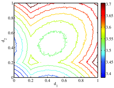
(a) Prior $\theta\sim\mathcal{U}(0,1)$

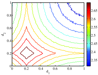
(b) Prior $\theta\sim\mathcal{U}(0,\theta_{e})$

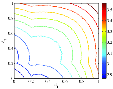
(c) Prior $\theta\sim\mathcal{U}(\theta_{e},1)$

Figure 3: Estimated expected utility for the design of two experiments with the simple nonlinear model, under different priors, where $\theta_{e}=\sqrt{\frac{1-e^{-0.8}}{2.88}}\approx 0.4373$.

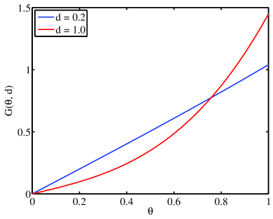
Figure 4: Noiseless output of the simple nonlinear model $G(\theta,d)$ as a function of the uncertain parameter $\theta$, at two designs: $d=0.2$ and $d=1$.

Again using a $\mathcal{U}(0,1)$ prior on $\theta$, the expected utility is plotted in Figure 3(a). First, note the symmetry in the contours along the $d_{1}=d_{2}$ line, which is expected since the two experiments have identical structure. Second, the optimal pair of experiments is not just a repeat of the optimal single-experiment design: $\mathbf{d}^{\ast}\neq(1,1)$, and instead we have $\mathbf{d}^{\ast}=(0.2,1.0)$ or $(1.0,0.2)$. Some insight can be obtained by examining Figure 4, which plots the single-experiment model output $G(\theta,d)$ as a function of the uncertain parameter $\theta$ at the two locally optimal designs: $d=0.2$ and $d=1$. Intuitively, a high slope of $G$ should be more informative for the inference of $\theta$, as the output is then more sensitive to variations in the input. The plot shows that neither design has a greater slope over the entire range of the prior $\theta\sim\mathcal{U}(0,1)$. Instead, the slope is greater for $\theta\in[0,\theta_{e}]$ with design $d=0.2$, and greater for $\theta\in[\theta_{e},1.0]$ with design $d=1.0$, where $\theta_{e}=\sqrt{\frac{1-e^{-0.8}}{2.88}}\approx 0.4373$.

Let us then examine the cases of “restricted” priors $\theta\sim\mathcal{U}(0,\theta_{e})$ and $\theta\sim\mathcal{U}(\theta_{e},1)$. Expected utilities for a single experiment, under either of these priors, are shown in Figures 2(b) and 2(c). The optimal design for $\mathcal{U}(0,\theta_{e})$ is at 0.2 and for $\mathcal{U}(\theta_{e},1)$ it is at 1.0, supporting intuition from the analysis of slopes. Next, the expected utilities of two experiments, under the restricted priors, are shown in Figures 3(b) and 3(c). Since in both cases, a single design point can give $G$ maximum slope over the entire restricted prior range of $\theta$, it is not surprising that the optimal pair of experiments involves repeating the respective single-experiment optima. In contrast, the lack of a “clear winner” over the full prior $\mathcal{U}(0,1)$ intuitively explains why a combination of different design conditions may yield more informative data overall. Note that we have only focused on the two local optima $d=0.2$ and $d=1$ from the original $\theta\sim\mathcal{U}(0,1)$ analysis, but it is possible that new local or globally optimal design points could emerge as the prior is changed.

6 Application: combustion kinetics

Experimental diagnostics play an essential role in the development and refinement of chemical kinetic models for combustion [81, 82]. Available diagnostics are often indirect, imprecise, and incomplete, leaving significant uncertainty in relevant rate parameters and thermophysical properties [83, 84, 53, 85]. Uncertainties are particularly acute when developing kinetic models for new combustion regimes or for fuels derived from new feedstocks, such as biofuels. Questions of experimental design—e.g., which species to interrogate and under what conditions—are thus of great practical importance in this context.

6.1 Model description

We demonstrate our optimal experimental design framework on shock tube ignition experiments, which are a canonical source of kinetic data. In a shock tube experiment, the mixture behind the reflected shock experiences a sharp rise in tempeature and pressure; if conditions are suitable, this mixture then ignites after some time, known as the ignition delay time. Ignition delays and other observables extracted from the experiment carry indirect information about the elementary chemical kinetic processes occurring in the mixture. These experiments are well described by the dynamics of a spatially homogeneous, adiabatic, constant-pressure chemical mixture.

We model the evolution of the mixture using ordinary differential equations (ODEs) expressing conservation of energy and of individual chemical species. Governing equations are detailed in C. We consider an initial mixture of hydrogen and oxygen. (Note that H₂-O₂ kinetics are a key subset of the reaction mechanisms associated with the combustion of complex hydrocarbons.) Our baseline kinetic model is a 19-reaction mechanism proposed in [86], reproduced in Table 1. Detailed chemical kinetics lead to a stiff set of nonlinear ODEs, with state variables consisting of temperature and species mass or molar fractions. The initial condition of the system is specified by the initial temperature $T_{0}$ and the fuel-oxidizer equivalence ratio $\phi$. Species production rates depend on the mixture conditions and on a set of kinetic parameters: pre-exponential factors $A_{m}$, temperature exponents $b_{m}$, and activation energies $E_{a,m}$, where $m$ is the reaction number in Table 1. These parameters are important in determining combustion characteristics and are of great interest in practice. Thermodynamic parameters and reaction rates in the governing equations are evaluated with the help of Cantera 1.7.0 [87, 88], an open-source chemical kinetics software package. ODEs are solved implicitly, using the variable-order backwards differentiation formulas implemented in CVODE [89].

6.2 Experimental goals

In this study, the experimental goal is to infer selected kinetic parameters ($A_{m}$, $b_{m}$, and $E_{a,m}$) associated with the elementary reactions in Table 1. For demonstration, we let the kinetic parameters of interest be $A_{1}$ and $E_{a,3}$. Reaction 1 is a chain-branching reaction, leading to a net increase in the number of radical species in the system. Reaction 3 is a chain-propagating reaction, exchanging one radical for another, but nonetheless relevant to the overall dynamics. We infer $\ln(A_{1}/A_{1}^{0})$ rather than $A_{1}$ directly, where $A_{1}^{0}$ is the nominal value of $A_{1}$ in [86]; this transformation ensures positivity and lets us easily impose a log-uniform prior on $A_{1}$, which is appropriate since the pre-exponential is a multiplicative factor. The design variables are the initial temperature $T_{0}$ and equivalence ratio $\phi$.

We once again use the expected utility defined in Equation (6) (and its estimator in Equation (9)) as the objective to be maximized for optimal design. Unlike the algebraic model in Section 5, however, this combustion problem offers many possible choices of observable. Some observables are more informative than others; we explore this choice in the next section.

6.3 Observables and likelihood function

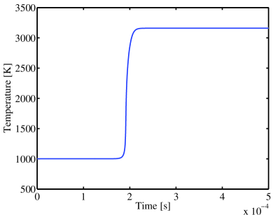
(a) Temperature

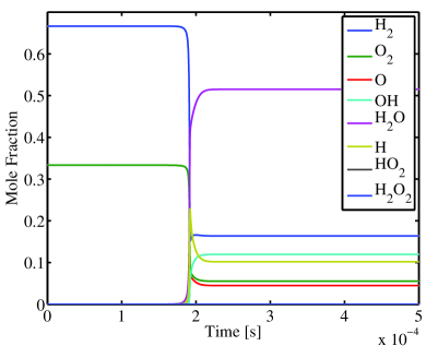
(b) Species molar fractions

Figure 5: Typical time-evolution of temperature and species molar fractions in H₂-O₂  ignition.

Typical trajectories of the state variables are shown in Figure 5. The temperature rises suddenly upon ignition; reactant species are rapidly consumed and product species are produced as the mixture comes to equilibrium. The most complete and detailed set of system observables are the state variables as a function of time. One could simply discretize the time domain to produce a finite-dimensional data vector $\mathbf{y}$. Too few discretization points might fail to capture the state behaviour, however. And because the kinetic parameters affect ignition delay, the state at any given time may have a nearly discontinuous dependence on the parameters. (This is due to the sharpness of the ignition front; at a fixed time, the state is most probably either pre-ignition or post-ignition.) Such a dependence makes construction of a polynomial chaos surrogate far more challenging [90]. It is desirable to transform the state into alternate observables that somehow “compress” the information and depend relatively smoothly on the kinetic parameters, while retaining features that are relevant to the experimental goals. We would also like to select observables that are easy to obtain experimentally.

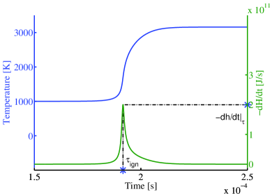
(a) $\tau_{ign}$

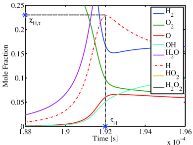
(b) $\tau_{H}$ and $X_{H,\tau}$

Figure 6: Illustration of the observables $\tau_{ign}$, $\tau_{H}$, and $X_{H,\tau}$ in the combustion problem.

Taking the above factors into consideration, we will use the observables in Table 2. The observables are the peak value of the heat release rate, the peak concentrations of various intermediate chemical species (O, H, HO₂, H₂O₂), and the times at which these peak values occur. Examples of $\tau_{ign}$, $\tau_{H}$, $\left.\frac{dh}{dt}\right|_{\tau}$, and $X_{H,\tau}$ are shown in Figure 6. The time of peak heat release coincides with the time at which temperature rises most rapidly. We thus take it as our definition of ignition delay, $\tau_{ign}$. We use the logarithm of all the characteristic time variables in our actual implementation, as the times are positive and vary over several orders of magnitude as a function of the kinetic parameters and design variables.

The likelihood is defined using the ODE model predictions and independent additive Gaussian measurement errors: $\mathbf{y}=\mathbf{G}(\bm{\theta},\mathbf{d})+\bm{\epsilon}$, with components $\epsilon_{c}\sim\mathcal{N}(0,\sigma^{2}_{c})$. For the concentration observables, the standard deviation of the measurement error is taken to be 10% of the value of the corresponding signal:

$$\sigma^{X}_{c}=0.1G_{c}(\bm{\theta},\mathbf{d}).$$ (42)

For the characteristic-time observables, we add a small constant $\alpha=10^{-5}$ s to the standard deviation, reflecting the minimum resolution of the timing technology:

$$\sigma^{\tau}_{c}=0.1G_{c}(\bm{\theta},\mathbf{d})+\alpha.$$ (43)

Note that the noise magnitude depends implicitly on both the kinetic parameters and the design variables. Both terms contributing to the expected information gain in Equation (8) are therefore influential, and one would expect a maximum entropy sampling approach to yield different results than the present experimental design methodology.

6.4 Polynomial chaos construction

Each solve of the ODE system defining $\mathbf{G}(\bm{\theta},\mathbf{d})$ is expensive, and thus we employ a polynomial chaos surrogate. In practice, since non-intrusive construction of the surrogate requires many forward model evaluations, the surrogate is only worth forming if the total number of model evaluations required for optimization of the expected utility exceeds the number required for surrogate construction. A detailed analysis of this tradeoff and the potential computational gains can be found in Section 6.7.

Uniform priors are assigned to the model parameters $\bm{\theta}\equiv\left[\ln(A_{1}/A_{1}^{0}),E_{a,3}\right]$ and uniform input distributions are assumed for the design variables $\left[T_{0},\phi\right]$ (see Section 3.1), with the supports given in Table 3. The polynomial chaos expansions thus use Legendre polynomials, with $\xi_{1},\xi_{2},\xi_{3},\xi_{4}\sim\mathcal{U}(-1,1)$. Our goal now is to construct PC expansions for the model outputs $\mathbf{G}(\bm{\theta},\mathbf{d})=(\ln\tau_{ign},\ln\tau_{O},\ln\tau_{H},\ln\tau_{HO_{2}},\ln\tau_{H_{2}O_{2}},$ $\left.\frac{dh}{dt}\right|_{\tau},X_{O,\tau},X_{H,\tau},X_{HO_{2},\tau},X_{H_{2}O_{2},\tau})$, using the projection given in Equation (27). For each desired PC coefficient, the numerator in that equation is evaluated using the modified DASQ algorithm described in Section 3.3. The expansions are truncated at a total order of $p=12$, and DASQ is stopped once a total of $n_{\mathrm{quad}}=10^{6}$ function evaluations have been exceeded. The degree of this expansion is admittedly (and deliberately) chosen rather high. The performance of lower-order expansions is examined below and in Section 6.7.

Indeed, the accuracy of the PC surrogate can be analyzed more rigorously by evaluating its relative $L^{2}$ error over a range of $p$ and $n_{\mathrm{quad}}$ values:

$$e_{c}=\frac{\int_{\bm{\Xi}}\left|G_{c}(\bm{\theta}(\bm{\xi}),\mathbf{d}(\bm{\xi}))-G_{c}^{p,n_{\mathrm{quad}}}(\bm{\xi})\right|^{2}p(\bm{\xi})\,d\bm{\xi}}{\int_{\bm{\Xi}}\left|G_{c}(\bm{\theta}(\bm{\xi}),\mathbf{d}(\bm{\xi}))\right|^{2}p(\bm{\xi})\,d\bm{\xi}},\qquad c=1\ldots n_{y}.$$ (44)

For the $c$th observable, $G_{c}$ is the output of the original ODE model and $G_{c}^{p,n_{\mathrm{quad}}}$ is the corresponding PC surrogate. $\bm{\theta}$ and $\mathbf{d}$ are affine functions of $\bm{\xi}$ (the PC expansions of the model inputs). Accurately evaluating the $L^{2}$ error is expensive, certainly more expensive than computing $G_{c}^{p,n_{\mathrm{quad}}}$ in the first place. But additional integration error must be minimized, and the integrals in Equation (44) are thus evaluated using a level-15 isotropic Clenshaw-Curtis sparse quadrature rule, containing 3,502,081 distinct abscissae.

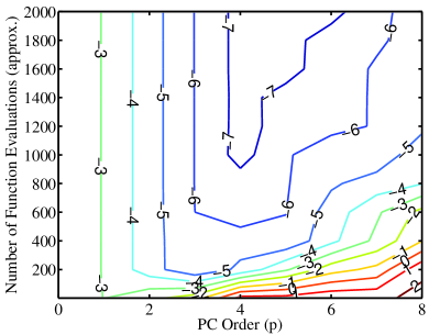
Figure 7: $\log_{10}$ of the $L^{2}$ error in the PC expansion for the peak heat release rate.

Figure 7 shows contours of $\log_{10}$ of the $L^{2}$ error over a range of $p$ and $n_{\mathrm{quad}}$, for the PC expansion of the peak enthalpy release rate. The $n_{\mathrm{quad}}$ values are approximate, as DASQ is terminated at the end of the iteration that exceeds $n_{\mathrm{quad}}$. When $n_{\mathrm{quad}}$ is too small, the error is dominated by aliasing (integration) error and increases with $p$. When a sufficiently large $n_{\mathrm{quad}}$ is used such that truncation error dominates, exponential convergence with respect to $p$ can be observed, as expected for smooth functions. Ideally, $n_{\mathrm{quad}}$ and $p$ should be selected at the “knees” of these contour plots, since little accuracy can be gained when $n_{\mathrm{quad}}$ is increased any further, but these locations can be difficult to pinpoint a priori.

6.5 Design of a single experiment

Figures 8(a) and 8(b) show contours of the expected utility estimates, $\hat{U}(\mathbf{d})$, in the two-dimensional design space, constructed using the full ODE model (with estimator parameters $n_{\mathrm{in}}=n_{\mathrm{out}}=10^{3}$) and the PC surrogate (with estimator parameters $n_{\mathrm{in}}=n_{\mathrm{out}}=10^{4}$), respectively. Contours from the PC surrogate are very similar to those from the full model, though the former have less variability due to the larger number of Monte Carlo samples used to compute $\hat{U}$. Most importantly, both plots yield the same optimal experimental design at around $(T_{0}^{\ast},\phi^{\ast})=(975,0.5)$.

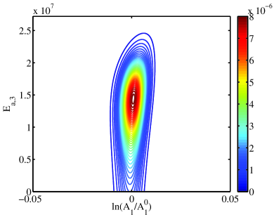
(a) Design $A$ full ODE model

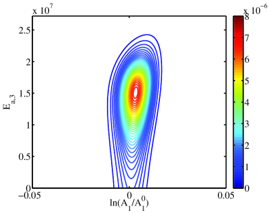
(b) Design $A$ PC surrogate

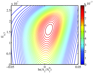
(c) Design $B$ full ODE model

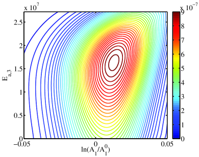
(d) Design $B$ PC surrogate

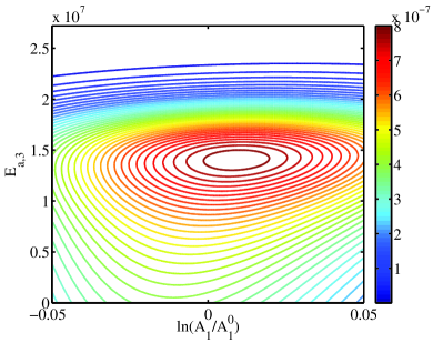
(e) Design $C$ full ODE model

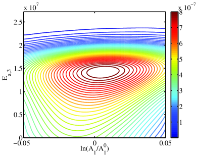
(f) Design $C$ PC surrogate

Figure 9: Contours of posterior density of the kinetic parameters, showing the results of inference with data obtained at three different experimental conditions (designs $A$, $B$, and $C$). Left column: posteriors constructed using the full ODE model; right column: posteriors constructed via the PC surrogate with $p=12$, $n_{\mathrm{quad}}=10^{6}$.

To test how well the expected information gain anticipates the performance of an experiment, the inference problem is solved at three different design points $A$, $B$, and $C$, listed in Table 4 and illustrated in Figure 8(b). Since the expected utility is highest at design $A$, then the posterior is expected to reflect the largest information gain at that experimental condition. We use the full ODE model to generate artificial data at each of the three design conditions, then perform inference. Contours of posterior density are shown in Figure 9, using the full ODE model and the PC surrogate. The posteriors of the full model and PC surrogate match very well; hence the PC surrogate is suitable not only for experimental design, but also for inference. As expected from the expected utility plots, the posterior distribution of the kinetic parameters is tightest at design $A$; this was the most informative of the three experimental conditions. Posterior modes of the ODE model and PC results are not precisely the same, however, due to the modeling error associated with the PC surrogate. Also, the posterior modes obtained with the full ODE model do not exactly match the values used to generate the artificial data, due to the noise in the likelihood model.

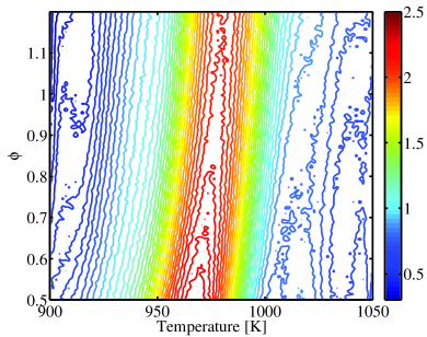
(a) All observables (same as Figure 8(b))

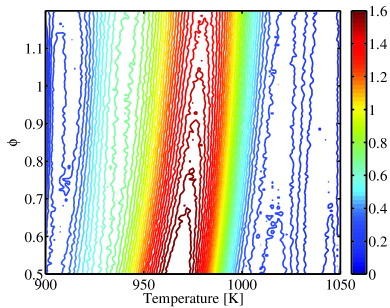
(b) Characteristic time observables

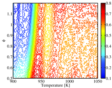
(c) Peak value observables

Figure 10: Estimated expected utility contours in the single-experiment combustion design problem using the PC surrogate with $p=12$ and $n_{\mathrm{quad}}=10^{6}$, but with different sets of observables.

What if a different set of observables are used? Two cases are explored: first, using only the characteristic time observables (i.e., the first five rows of Table 2); and second, using only the peak value observables (i.e., the last five rows of Table 2). The corresponding expected utility plots are given in Figure 10 (using the PC surrogate only). Several remarks can be made. First, the characteristic time observables are more informative than the peak value observables, as demonstrated by the higher expected utility values in Figure 10(b) than Figure 10(c). Second, the choice of observables can greatly influence the optimal value of the design parameters. Third, even though the observables from the two cases form a partition of the full observable set, their expected utility values do not simply sum to that of the full-observable case. (This is a special case of the analysis in A.) The lesson is that the selection of appropriate observables is a very important part of the design procedure, especially if one is forced to select only a few modes of observation. This selection could be made into an argument of the objective function, augmenting $\mathbf{d}$ and leading to a mixed-integer optimization problem.

6.6 Design of two experiments: stochastic optimization

Now we perform a study analogous to that in Section 5.2, designing two ignition experiments (of the same structure) simultaneously. The experimental goal of inferring $A_{1}$ and $E_{a,3}$ is unchanged, and for computational efficiency we use only the $p=12$, $n_{\mathrm{quad}}=10^{6}$ PC surrogate. The design space is now four-dimensional, with $\mathbf{d}=[T_{0,1},\phi_{1},T_{0,2},\phi_{2}]$. Stochastic optimization is used to find the optimal experimental design, as a grid search is entirely impractical.

Coupling stochastic optimization schemes (Section 2.4) with the estimator $\hat{U}(\mathbf{d})$ of expected information gain introduces a few new numerical tradeoffs. The number of samples in the outer loop of the estimator controls the variance of $\hat{U}$, which dictates the noise level of the objective function. Lower noise in the objective function might imply fewer optimization iterations overall, while a noisier objective may require many more iterations of either SPSA or NMNS to make progress towards the optimum. On the other hand, noise should not be reduced too much for SPSA, since the usefulness of its gradient approximation relies on the existence of a non-negligible noise level. In general, the task of balancing $n_{\mathrm{out}}$ against the number of optimization iterations, in order to minimize the number of model evaluations, is not trivial. We therefore test different values of $n_{\mathrm{out}}$ to understand their impact on the SPSA and NMNS optimization schemes. We fix $n_{\mathrm{in}}$ at $10^{4}$ in order to maintain a low bias contribution from the inner loop.

Since the results of stochastic optimization are themselves random, we use an ensemble of 100 independent optimization runs at any given parameter setting to analyze performance. Each optimization run is capped at $n_{\mathrm{noisyObj}}=10^{4}$ evaluations of the noisy objective—i.e., of the summand in Equation (9)—where each noisy objective evaluation itself involves $n_{\mathrm{in}}$ evaluations of the model $\mathbf{G}$ or the surrogate $\mathbf{G}^{p}$. We can thus compare performance at a fixed computational cost.

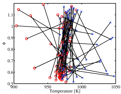
(a) SPSA $n_{\mathrm{out}}=1$

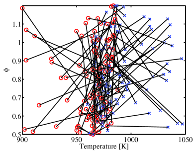
(b) NMNS $n_{\mathrm{out}}=1$

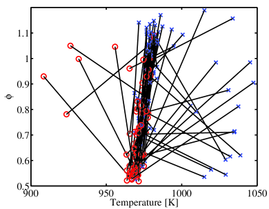
(c) SPSA $n_{\mathrm{out}}=10$

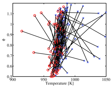
(d) NMNS $n_{\mathrm{out}}=10$

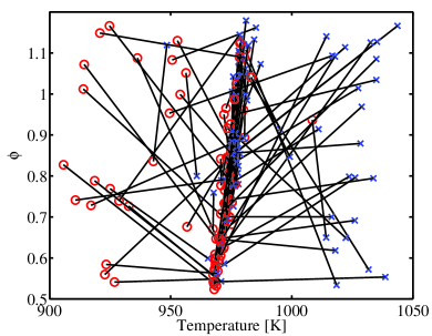
(e) SPSA $n_{\mathrm{out}}=100$

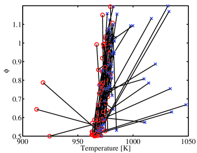
(f) NMNS $n_{\mathrm{out}}=100$

Figure 11: Two-experiment combustion design problem: final outputs from 100 independent runs of stochastic optimization, using SPSA and NMNS with a limit of $n_{\mathrm{noisyObj}}=10^{4}$, and with different numbers of outer Monte Carlo iterations, using the PC surrogate with $p=12$, $n_{\textrm{quad}}=10^{6}$.

Runs are performed for both SPSA and NMNS, with $n_{\mathrm{out}}$ ranging from 1 to 100. The final design conditions and convergence histories (the latter plotted for 10 runs only) are shown in Figures 11 and 12, respectively. In Figure 11, each connected blue cross and red circle represent a pair of final experimental designs, where the red circle is arbitrarily chosen to represent the lower $T_{0}$ design. The optimization results indicate that both experiments should be performed near $T_{0}=975$ K, although the best $\phi$ is less precisely determined and less influential. This pattern is similar to that of a single-experiment optimal design. Overall, a tighter clustering of the final design points is observed as $n_{\mathrm{out}}$ is increased. SPSA groups the majority of the final design points more tightly, but it also yields more outliers than NMNS; in other words, it results in more of a “hit-or-miss” situation. Figure 11 indicates that, for the NMNS cases, a lower $n_{\mathrm{out}}$ lets the algorithm reach the convergence “plateau” more quickly. This result is affected both by the shrinkage rate of the simplex and by the fact that a higher $n_{\mathrm{out}}$ simply requires more model evaluations even to complete one iteration. The choice of $n_{\mathrm{out}}$ then should take into consideration how many model evaluations are available. Even then, the best choice may depend on the shape of the expected utility surface and the variance of its estimator (which is not stationary in $\mathbf{d}$).

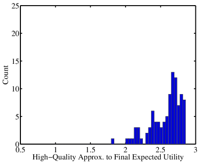
(a) SPSA $n_{\mathrm{out}}=1$

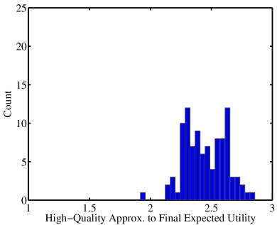
(b) NMNS $n_{\mathrm{out}}=1$

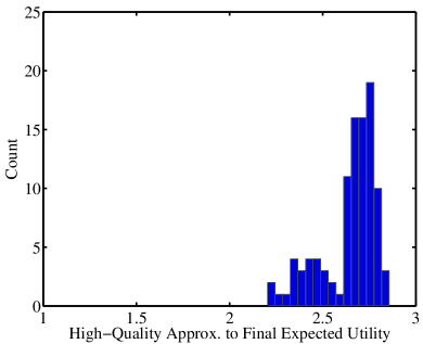
(c) SPSA $n_{\mathrm{out}}=10$

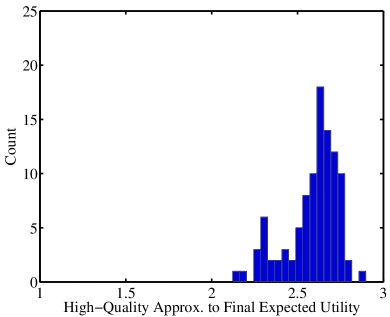
(d) NMNS $n_{\mathrm{out}}=10$

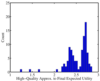
(e) SPSA $n_{\mathrm{out}}=100$

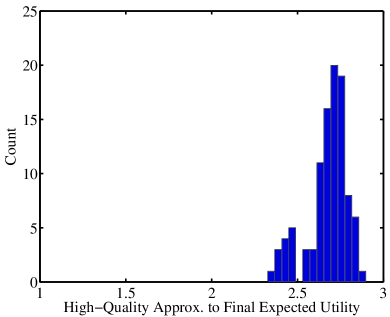
(f) NMNS $n_{\mathrm{out}}=100$

Figure 13: High-quality expected utility estimates corresponding to the optimization outputs in Figure 11. Each high-quality estimate is based on $n_{\mathrm{out}}=n_{\mathrm{in}}=10^{4}$ samples.

Our observations so far are based on an assessment of the design locations and convergence history. A more quantitative analysis should focus on the expected utility value of the final designs, which is what really matters in the end. Figure 13 shows histograms of expected utility for the 100 final design points resulting from each optimization case. To compare the design points, we want to make the error incurred in estimating $U(\mathbf{d}^{\ast})$ relatively negligible, and thus we employ a high-quality estimator with $n_{\mathrm{out}}=n_{\mathrm{in}}=10^{4}$. This is not the small-sample estimator used inside the optimization algorithms; it is a more expensive estimator used afterwards, only for diagnostic purposes. The histograms indicate that increasing $n_{\mathrm{out}}$ is actually not very effective for SPSA, as the persistence of outliers creates a spread in the final values, supporting our suspicion that too small a noise level may be bad for SPSA. On the other hand, increasing $n_{\mathrm{out}}$ is effective for NMNS. The bimodal structure of the histograms is due to the two groups: good designs on the center “ridge” and outliers, with few designs having expected utility values in between. Overall, NMNS performs better than SPSA in this study, both in terms of the asymptotic distribution of design parameters and how quickly the convergence plateau or “knee” is reached.

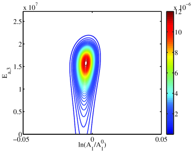
(a) Design $D$

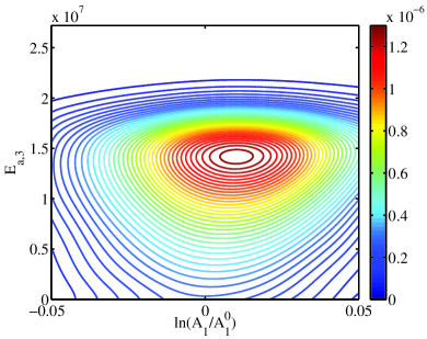
(b) Design $E$

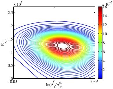
(c) Design $F$

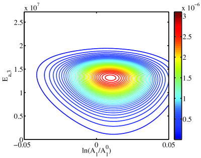
(d) Design “factorial”

Figure 14: Posterior densities resulting from inference at the experimental conditions listed in Table 5, using the PC surrogate with $p=12$, $n_{\textrm{quad}}=10^{6}$.

To validate the results, the parameter inference problem is solved with data from three two-experiment design points (labeled $D$, $E$, and $F$) and with data from a four-experiment factorial design. All of the experimental conditions are listed in Table 5. Design $D$, a pair of experiments lying on the ridge of “good designs,” is expected to have the tightest posterior among the two-experiment designs. The posteriors are shown in Figure 14, using the PC surrogate only. Indeed, design $D$ has the tightest posterior, and is much better than the four-experiment factorial design even though it uses fewer experiments! The factorial design blindly picks all the corners in the design space, which are in general not good design points. (The number of experiments in a factorial design would also increase exponentially with the number of design parameters, becoming impractical very quickly.) Model-based optimal experimental design is far more robust and capable than this traditional method.

6.7 Is using a PC surrogate worthwhile?

In producing the previous results, we used a PC surrogate with $p=12$ and $n_{\mathrm{quad}}=10^{6}$, though analysis for one observable in Figure 7 suggests that this polynomial truncation and adapted quadrature rule are perhaps of higher quality than necessary for our problem. To quantitatively determine whether a polynomial surrogate offers efficiency gains in this study (or any other), we must (i) check if a lower quality PC surrogate may be used while still achieving results of similar quality, and (ii) analyze the computational cost.

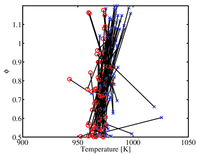
(a) Final positions

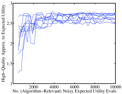
(b) Convergence history

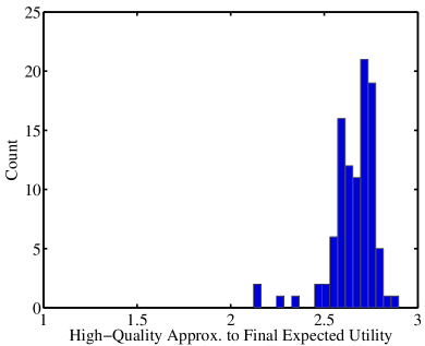
(c) Final expected utilities

Figure 15: Two-experiment combustion design problem: final outputs from 100 independent runs of stochastic optimization. Optimization is performed using only a lower-order PC surrogate ($p=6$ and $n_{\mathrm{quad}}=10^{4}$). To report performance, the expected utility estimates in subfigures (b) and (c) are computed using a higher-order PC surrogate ($p=12$ and $n_{\mathrm{quad}}=10^{6}$) and $n_{\mathrm{out}}=n_{\mathrm{in}}=10^{4}$ samples. Only results with NMNS and $n_{\mathrm{out}}=100$ are shown. Compare to Figures 11(f), 12(f), and 13(f).

To check if a lower-quality PC surrogate would suffice, the same two-experiment optimal experimental design problem is solved but now with $p=6$. We find that $n_{\mathrm{quad}}=10^{4}$ is roughly the smallest $n_{\mathrm{quad}}$ that still yields reasonable results. The final optimization positions (obtained via NMNS only), the convergence history, and histogram of final expected utilities are shown in Figure 15. In fact, the histogram appears to be even tighter than that obtained with the $p=12$ surrogate.

To analyze the computational cost, we assume that optimization is terminated after 5000 noisy objective function evaluations, as the practical convergence plateau is reached by that point. If each noisy objective function requires $10^{4}$ inner Monte Carlo samples and each PC evaluation is negligible compared to full model, then using the full ODE model requires $5000\times 10^{4}=5\times 10^{7}$ model evaluations, whereas the construction of the PC surrogate requires $10^{4}$ full ODE model evaluations. The surrogate thus provides a speedup of roughly 3.5 orders of magnitude, saving 49,990,000 full model evaluations (roughly 4 months of computational time for the present problem, if run serially).

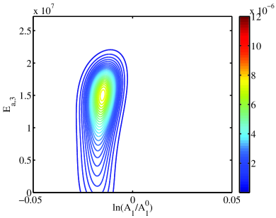
(a) Design $D$

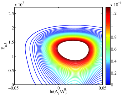
(b) Design $E$

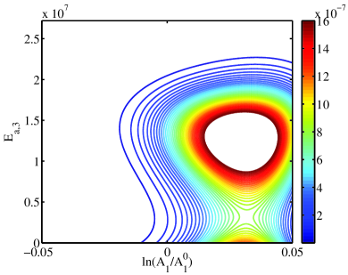
(c) Design $F$

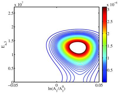
(d) Design “factorial”

Figure 16: Posterior densities resulting from inference at the experimental conditions listed in Table 5, using a lower-order PC surrogate with $p=6$, $n_{\textrm{quad}}=10^{4}$. Compare to Figure 14.

Even though a low-quality surrogate may be sufficient for optimal experimental design, it may not be sufficiently accurate for parameter inference. For example, the two-experiment and four-experiment posteriors obtained using the $p=6$, $n_{\mathrm{quad}}=10^{4}$ surrogate are shown in Figure 16. These posterior density contours show a substantial loss of accuracy compared to the corresponding plots in Figure 14. Because inference does not involve averaging over the data space and broadly exploring the design space, and because it generally favors a more restricted range of the model parameters $\bm{\theta}$, it may be more sensitive to local errors than the optimal experimental design formulation. There are two possible solutions to this issue:

1. Build and use a high-order polynomial chaos surrogate at the outset of analysis, and use it for both optimal experimental design and inference. Because inference typically employs MCMC and thus requires many thousands or even millions of model evaluations, the combined computational savings will make such a surrogate almost certainly worth constructing.

2. A more efficient approach is to use a low-order polynomial chaos expansion to perform the optimal experimental design. Upon reaching the optimal design conditions, construct a new PC expansion for inference at that design only. The new expansion does not need to capture dependence on the design variables, and thus it involves a smaller dimension and fewer interactions. This less expensive local PC expansion can more easily be made sufficiently accurate for the inference problem.

7 Conclusions

This paper presents a systematic framework and a set of computational tools for the optimal design of experiments. The framework can incorporate nonlinear and computationally intensive models of the experiment, linking them to rigorous information theoretic design criteria and requiring essentially no simplifying assumptions. A flowchart of the overall framework is given in Figure 1, showing the steps of optimal design and their role in a larger design–experimentation–model improvement cycle.

We focus on the experimental goal of parameter inference, in a Bayesian statistical setting, where a good design criterion is shown to maximize expected information gain from prior to posterior. A two-stage Monte Carlo estimator of expected information gain is coupled to algorithms for stochastic optimization. The estimation of expected information gain, which would otherwise be prohibitive with computationally intensive models, is substantially accelerated through the use of flexible and accurate polynomial chaos surrogate representations.

We demonstrate our method first on a simple nonlinear algebraic model, then on shock tube ignition experiments described by a stiff system of nonlinear ODEs. The latter system is challenging to approximate, as certain model observables depend sharply on the combustion kinetic parameters and design conditions, and ignition delays vary over several orders of magnitude. In both these examples, we illustrate the design of single and multiple experiments. We analyze the impact of prior information on the optimal designs, and examine the selection of observables according to their information value. We also investigate numerical tradeoffs between variance in the estimator of expected utility and performance of the stochastic optimization schemes.

Overall we find that inference at optimal design conditions is indeed very informative about the targeted parameters, and that model-based optimal experiments are far more informative than those obtained with simple heuristics. The use of surrogates offers significant computational savings over stochastic optimization with the full model, more than three orders of magnitude in the examples tested here. Moreover, we find that the polynomial surrogate used in optimal experimental design need not be extremely accurate in order to reveal the correct design points; surrogate requirements for optimal design are less stringent than for parameter inference.

Several promising avenues exist for future work. More efficient means of constructing polynomial chaos expansions, adaptively and in conjunction with stochastic optimization, may offer considerable computational gains. Uncertainty in the design parameters themselves can also be incorporated into the framework, as in real-world experiments where the design conditions cannot be precisely imposed; this additional uncertainty could be treated with a hierarchical Bayesian approach. Structural inadequacy of the model $\mathbf{G}$ is another important issue; how successful is an “optimal” design (or indeed an inference process) based on a forward model that cannot fully resolve the physical processes at hand? Our current experience on design with lower-order polynomial surrogates provides a glimpse into issues of structural uncertainty, but a much more thorough exploration is needed. Finally, the Bayesian optimal design methodology has a natural extension to sequential experimental design, where one set of experiments can be performed and analyzed before designing the next set. A rigorous approach to sequential design, incorporating ideas from dynamic programming and perhaps sequential Monte Carlo, may be quite effective.

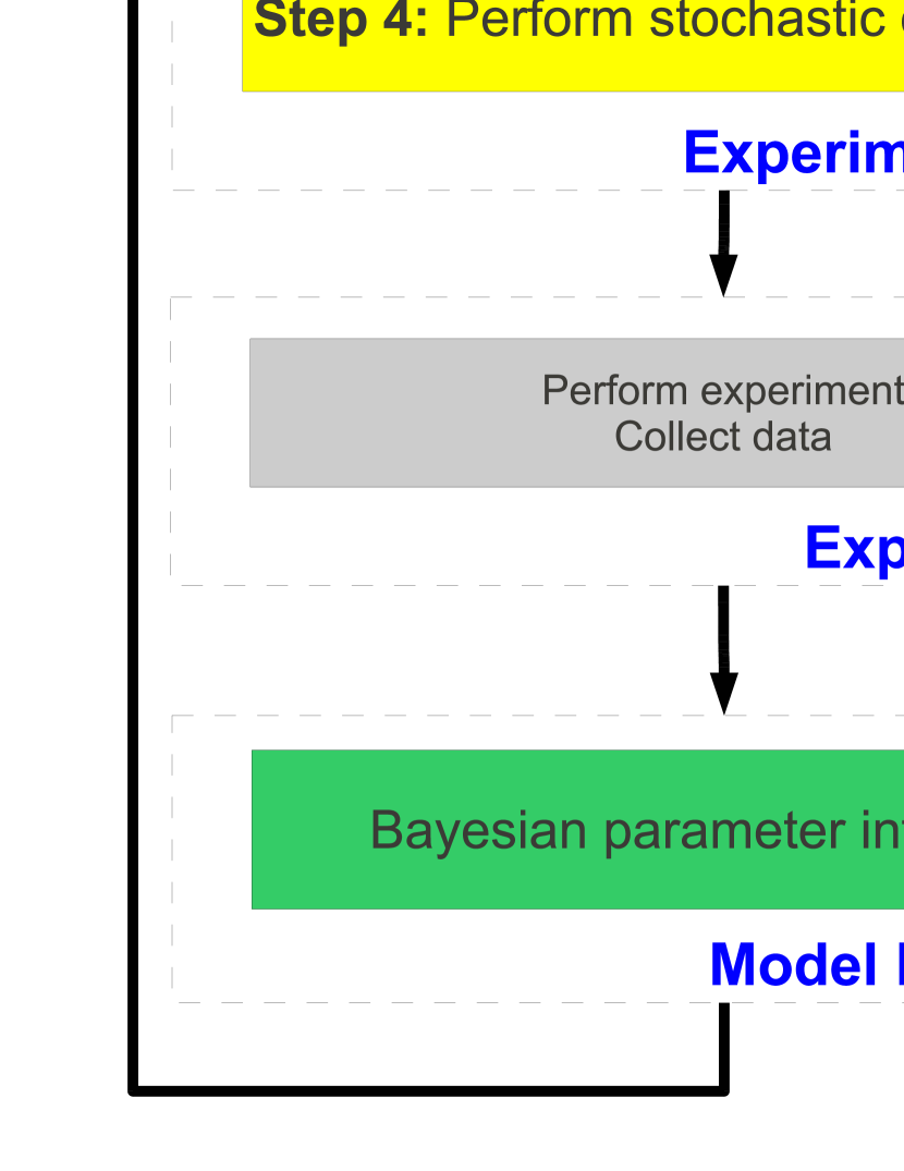
Figure 1: A flowchart summarizing the key steps of the design–experimentation–model improvement cycle.

$\mathbf{i}=(1,\cdots,1)$;

$\mathcal{O}=\emptyset$;

$\mathcal{A}=\{\mathbf{i}\}$;

for $r=1$ to $n_{\mathrm{coef}}$ do

       $v_{r}=\Delta_{\mathbf{i}}f_{r}$;

       Compute $h_{r,\mathbf{i}}$;

      

end for

$\eta=\bar{h}_{\mathbf{i}}$. For example, $\bar{h}_{\mathbf{i}}=\max_{r}h_{r,\mathbf{i}}$;

while $\eta>$ TOL do

       select $\mathbf{i}$ from $\mathcal{A}$ with the largest $\bar{h}_{\mathbf{i}}$;

       $\mathcal{A}=\mathcal{A}\setminus\{\mathbf{i}\}$;

       $\mathcal{O}=\mathcal{O}\cup\{\mathbf{i}\}$;

       $\eta=\eta-\bar{h}_{\mathbf{i}}$;

       for $p=1$ to $d$ do

             $\mathbf{j}=\mathbf{i}+\mathbf{e}_{p}$;

             if $\mathbf{j}-\mathbf{e}_{q}\in\mathcal{O}$ for all $q=1,\cdots,d$ then

                   $\mathcal{A}=\mathcal{A}\cup\{\mathbf{j}\}$;

                   for $r=1$ to $n_{\mathrm{coef}}$ do

                         $s_{r}=\Delta_{\mathbf{j}}f_{r}$;

                         $v_{r}=v_{r}+s_{r}$;

                         Compute $h_{r,\mathbf{j}}$;

                        

                   end for

                  Compute $\bar{h}_{\mathbf{j}}$;

                   $\eta=\eta+\bar{h}_{\mathbf{j}}$;

                  

             end if

            

       end for

      

end while

Symbols:

$\mathcal{O}$—old index set;

$\mathcal{A}$—active index set;

$v_{r}$—computed integral value $\sum_{\mathbf{i}\in\mathcal{O}\cup\mathcal{A}}\otimes_{p=1}^{d}\Delta_{i_{p}}f_{r}$ for the $r$th coefficient;

$\Delta_{\mathbf{i}}f_{r}$—integral increment $\otimes_{p=1}^{d}\Delta_{i_{p}}f_{r}$ for the $r$th coefficient;

$h_{r,\mathbf{i}}$—local error indicator for the $r$th coefficient;

$\bar{h}_{\mathbf{i}}$—total effect local error indicator;

$\eta$—global error estimate $\sum_{\mathbf{i}\in\mathcal{A}}\bar{h}_{\mathbf{i}}$;

$TOL$—error tolerance;

$\mathbf{e}_{p}$—$p$th unit vector;

Algorithm 1 Modified dimension-adaptive sparse quadrature algorithm for non-intrusive spectral projection.

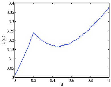
(a) Prior $\theta\sim\mathcal{U}(0,1)$

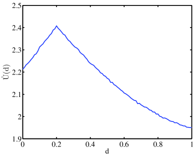
(b) Prior $\theta\sim\mathcal{U}(0,\theta_{e})$

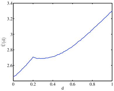
(c) Prior $\theta\sim\mathcal{U}(\theta_{e},1)$

Figure 2: Estimated expected utility for the design of a single experiment with the simple nonlinear model under different priors, where $\theta_{e}=\sqrt{\frac{1-e^{-0.8}}{2.88}}\approx 0.4373$.

Reaction No.	Elementary Reaction
R1	$\mathbf{H+O_{2}}$	$\mathbf{\Longleftrightarrow}$	$\mathbf{O+OH}$
R2	$O+H_{2}$	$\Longleftrightarrow$	$H+OH$
R3	$\mathbf{H_{2}+OH}$	$\mathbf{\Longleftrightarrow}$	$\mathbf{H_{2}O+H}$
R4	$OH+OH$	$\Longleftrightarrow$	$O+H_{2}O$
R5	$H_{2}+M$	$\Longleftrightarrow$	$H+H+M$
R6	$O+O+M$	$\Longleftrightarrow$	$O_{2}+M$
R7	$O+H+M$	$\Longleftrightarrow$	$OH+M$
R8	$H+OH+M$	$\Longleftrightarrow$	$H_{2}O+M$
R9	$H+O_{2}+M$	$\Longleftrightarrow$	$HO_{2}+M$
R10	$HO_{2}+H$	$\Longleftrightarrow$	$H_{2}+O_{2}$
R11	$HO_{2}+H$	$\Longleftrightarrow$	$OH+OH$
R12	$HO_{2}+O$	$\Longleftrightarrow$	$O_{2}+OH$
R13	$HO_{2}+OH$	$\Longleftrightarrow$	$H_{2}O+O_{2}$
R14	$HO_{2}+HO_{2}$	$\Longleftrightarrow$	$H_{2}O_{2}+O_{2}$
R15	$H_{2}O_{2}+M$	$\Longleftrightarrow$	$OH+OH+M$
R16	$H_{2}O_{2}+H$	$\Longleftrightarrow$	$H_{2}O+OH$
R17	$H_{2}O_{2}+H$	$\Longleftrightarrow$	$HO_{2}+H_{2}$
R18	$H_{2}O_{2}+O$	$\Longleftrightarrow$	$OH+HO_{2}$
R19	$H_{2}O_{2}+OH$	$\Longleftrightarrow$	$HO_{2}+H_{2}O$

Table 1: 19-reaction hydrogen-oxygen mechanism [86]. Reactions involving the wildcard species $M$ are three-body interactions, with different efficiencies for different species. Kinetic parameters of the boldface reactions are targeted for inference.

Observable	Explanation
$\tau_{ign}$	Ignition delay, defined as the time of peak enthalpy release rate
$\tau_{O}$	Characteristic time in which peak $X_{O}$ occurs
$\tau_{H}$	Characteristic time in which peak $X_{H}$ occurs
$\tau_{HO_{2}}$	Characteristic time in which peak $X_{HO_{2}}$ occurs
$\tau_{H_{2}O_{2}}$	Characteristic time in which peak $X_{H_{2}O_{2}}$ occurs
$\left.\frac{dh}{dt}\right|_{\tau}$	Peak value of enthalpy release rate
$X_{O,\tau}$	Peak value of $X_{O}$
$X_{H,\tau}$	Peak value of $X_{H}$
$X_{HO_{2},\tau}$	Peak value of $X_{HO_{2}}$
$X_{H_{2}O_{2},\tau}$	Peak value of $X_{H_{2}O_{2}}$

Table 2: Selected observables for the combustion problem. Note that $dh/dt<0$ when enthalpy is released or lost by the system.

Parameter	Lower Bound	Upper Bound
$\ln(A_{1}/A_{1}^{0})$	$-0.05$	0.05
$E_{a,3}$	0	$2.7196\times 10^{7}$
$T_{0}$	900	1050
$\phi$	0.5	1.2

Table 3: Prior support of the uncertain kinetic parameters $\ln(A_{1}/A_{1}^{0})$ and $E_{a,3}$, and ranges of the design variables $T_{0}$ and $\phi$. A uniform prior is assigned to the kinetic parameters.

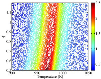
(a) Full ODE model

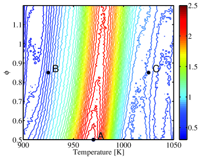
(b) PC surrogate

Figure 8: Estimated expected utility contours in the single-experiment combustion design problem, with design variables $T_{0}$ and $\phi$, using the full ODE model and the PC surrogate with $p=12$ and $n_{\mathrm{quad}}=10^{6}$. Inference problems are then solved at experimental conditions $A$, $B$, and $C$ to validate the experimental design procedure.

Design Point	$T_{0}$	$\phi$
$A$	975	0.5
$B$	925	0.85
$C$	1025	0.85

Table 4: Experimental conditions at design points $A$, $B$, and $C$.

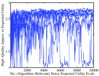
(a) SPSA $n_{\mathrm{out}}=1$

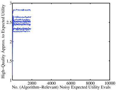
(b) NMNS $n_{\mathrm{out}}=1$

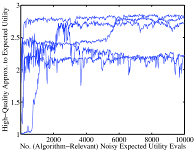
(c) SPSA $n_{\mathrm{out}}=10$

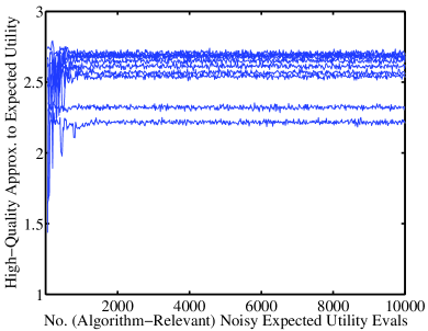
(d) NMNS $n_{\mathrm{out}}=10$

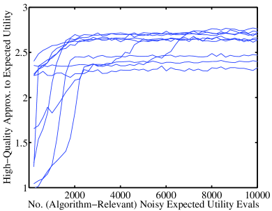
(e) SPSA $n_{\mathrm{out}}=100$

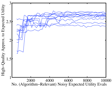
(f) NMNS $n_{\mathrm{out}}=100$

Figure 12: High-quality expected utility estimates, shown over the course of 10 independent stochastic optimization runs for the two-experiment combustion design. Each high-quality estimate is based on $n_{\mathrm{out}}=n_{\mathrm{in}}=10^{4}$ samples. Note that the output for NMNS $n_{\mathrm{out}}=1$ terminates earlier than the other cases because its simplices have already shrunk to sizes below machine precision.

Design Point	$T_{0,1}$	$\phi_{1}$	$T_{0,2}$	$\phi_{2}$	$T_{0,3}$	$\phi_{3}$	$T_{0,4}$	$\phi_{4}$
$D$	970	0.6	975	1.1	–	–	–	–
$E$	900	0.5	1050	1.2	–	–	–	–
$F$	900	1.2	1050	0.5	–	–	–	–
“factorial”	900	0.5	900	1.2	1050	0.5	1050	1.2

Table 5: Experimental conditions at design points $D$, $E$, $F$, and for a four-point factorial design.

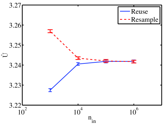
Figure 17: Expected utility estimates $\hat{U}(d=0.2)$ for the simple nonlinear problem in Section 2.3, using different sample sizes $n_{\mathrm{in}}$. One estimator (blue solid line) reuses samples between the inner/outer Monte Carlo loops while the other (red dashed line) does not. Errors bars show the mean and standard deviation of the sampling distribution of each estimator.

Appendix A Expected information gain from two experiments

Here we show that the expected information gain from two experiments is not, in general, equal to the sum of the expected information gains due to each experiment individually.

Consider two fixed experimental conditions $\mathbf{d}_{1}$ and $\mathbf{d}_{2}$, with corresponding data $\mathbf{y}_{1}$ and $\mathbf{y}_{2}$. Following Equation (6), the expected information gain in the model parameters $\bm{\theta}$ from performing both experiments is

$$U([\mathbf{d}_{1},\mathbf{d}_{2}]) = \int_{\mathcal{Y}_{1}}\int_{\mathcal{Y}_{2}}\int_{\bm{\Theta}}p(\bm{\theta}|\mathbf{y}_{1},\mathbf{y}_{2},\mathbf{d}_{1},\mathbf{d}_{2})\ln\left[\frac{p(\bm{\theta}|\mathbf{y}_{1},\mathbf{y}_{2},\mathbf{d}_{1},\mathbf{d}_{2})}{p(\bm{\theta})}\right]\,d\bm{\theta}\,p(\mathbf{y}_{1},\mathbf{y}_{2}|\mathbf{d}_{1},\mathbf{d}_{2})\,d\mathbf{y}_{2}\,d\mathbf{y}_{1}$$ (45)

$$= \int_{\mathcal{Y}_{1}}\int_{\mathcal{Y}_{2}}\int_{\bm{\Theta}}\ln\left[\frac{p(\mathbf{y}_{1},\mathbf{y}_{2}|\bm{\theta},\mathbf{d}_{1},\mathbf{d}_{2})}{p(\mathbf{y}_{1},\mathbf{y}_{2}|\mathbf{d}_{1},\mathbf{d}_{2})}\right]p(\mathbf{y}_{1},\mathbf{y}_{2}|\bm{\theta},\mathbf{d}_{1},\mathbf{d}_{2})p(\bm{\theta})\,d\bm{\theta}\,d\mathbf{y}_{2}\,d\mathbf{y}_{1}$$

$$= \int_{\mathcal{Y}_{1}}\int_{\bm{\Theta}}\ln\left[p(\mathbf{y}_{1}|\bm{\theta},\mathbf{d}_{1})\right]p(\mathbf{y}_{1}|\bm{\theta},\mathbf{d}_{1})p(\bm{\theta})\,d\bm{\theta}\,d\mathbf{y}_{1}$$

$$+\int_{\mathcal{Y}_{2}}\int_{\bm{\Theta}}\ln\left[p(\mathbf{y}_{2}|\bm{\theta},\mathbf{d}_{2})\right]p(\mathbf{y}_{2}|\bm{\theta},\mathbf{d}_{2})p(\bm{\theta})\,d\bm{\theta}\,d\mathbf{y}_{2}$$

$$-\int_{\mathcal{Y}_{1}}\int_{\mathcal{Y}_{2}}\int_{\bm{\Theta}}\ln\left[p(\mathbf{y}_{1},\mathbf{y}_{2}|\mathbf{d}_{1},\mathbf{d}_{2})\right]p(\mathbf{y}_{1},\mathbf{y}_{2}|\bm{\theta},\mathbf{d}_{1},\mathbf{d}_{2})p(\bm{\theta})\,d\bm{\theta}\,d\mathbf{y}_{2}\,d\mathbf{y}_{1}$$

$$= \int_{\mathcal{Y}_{1}}\int_{\bm{\Theta}}\ln\left[p(\mathbf{y}_{1}|\bm{\theta},\mathbf{d}_{1})\right]p(\mathbf{y}_{1}|\bm{\theta},\mathbf{d}_{1})p(\bm{\theta})\,d\bm{\theta}\,d\mathbf{y}_{1}$$

$$+\int_{\mathcal{Y}_{2}}\int_{\bm{\Theta}}\ln\left[p(\mathbf{y}_{2}|\bm{\theta},\mathbf{d}_{2})\right]p(\mathbf{y}_{2}|\bm{\theta},\mathbf{d}_{2})p(\bm{\theta})\,d\bm{\theta}\,d\mathbf{y}_{2}$$

$$+h(\mathbf{y}_{1},\mathbf{y}_{2}|\mathbf{d}_{1},\mathbf{d}_{2}),$$

where the second equality is due to application of Bayes’ Theorem; the third equality uses the fact that $p(\mathbf{y}_{1},\mathbf{y}_{2}|\bm{\theta},\mathbf{d}_{1},\mathbf{d}_{2})=p(\mathbf{y}_{1}|\bm{\theta},\mathbf{d}_{1})p(\mathbf{y}_{2}|\bm{\theta},\mathbf{d}_{2})$, since the outputs are conditionally independent given the designs and parameters, and data from each experiment depend only on its own design given the parameters; and the last equality results from the marginalization of $\bm{\theta}$ to obtain the differential entropy $h$.

Similarly, the sum of the expected information gain due to each experiment individually is

$$U(\mathbf{d}_{1})+U(\mathbf{d}_{2}) = \int_{\mathcal{Y}_{1}}\int_{\bm{\Theta}}p(\bm{\theta}|\mathbf{y}_{1},\mathbf{d}_{1})\ln\left[\frac{p(\bm{\theta}|\mathbf{y}_{1},\mathbf{d}_{1})}{p(\bm{\theta})}\right]\,d\bm{\theta}\,p(\mathbf{y}_{1}|\mathbf{d}_{1})\,d\mathbf{y}_{1}$$ (46)

$$+\int_{\mathcal{Y}_{2}}\int_{\bm{\Theta}}p(\bm{\theta}|\mathbf{y}_{2},\mathbf{d}_{2})\ln\left[\frac{p(\bm{\theta}|\mathbf{y}_{2},\mathbf{d}_{2})}{p(\bm{\theta})}\right]\,d\bm{\theta}\,p(\mathbf{y}_{2}|\mathbf{d}_{2})\,d\mathbf{y}_{2}$$

$$= \int_{\mathcal{Y}_{1}}\int_{\bm{\Theta}}\ln\left[\frac{p(\mathbf{y}_{1}|\bm{\theta},\mathbf{d}_{1})}{p(\mathbf{y}_{1}|\mathbf{d}_{1})}\right]p(\mathbf{y}_{1}|\bm{\theta},\mathbf{d}_{1})\,p(\bm{\theta})\,d\bm{\theta}\,d\mathbf{y}_{1}$$

$$+\int_{\mathcal{Y}_{2}}\int_{\bm{\Theta}}\ln\left[\frac{p(\mathbf{y}_{2}|\bm{\theta},\mathbf{d}_{2})}{p(\mathbf{y}_{2}|\mathbf{d}_{2})}\right]p(\mathbf{y}_{2}|\bm{\theta},\mathbf{d}_{2})\,p(\bm{\theta})\,d\bm{\theta}\,d\mathbf{y}_{2}$$

$$= \int_{\mathcal{Y}_{1}}\int_{\bm{\Theta}}\ln\left[p(\mathbf{y}_{1}|\bm{\theta},\mathbf{d}_{1})\right]p(\mathbf{y}_{1}|\bm{\theta},\mathbf{d}_{1})p(\bm{\theta})\,d\bm{\theta}\,d\mathbf{y}_{1}$$

$$+\int_{\mathcal{Y}_{2}}\int_{\bm{\Theta}}\ln\left[p(\mathbf{y}_{2}|\bm{\theta},\mathbf{d}_{2})\right]p(\mathbf{y}_{2}|\bm{\theta},\mathbf{d}_{2})p(\bm{\theta})\,d\bm{\theta}\,d\mathbf{y}_{2}$$

$$-\int_{\mathcal{Y}_{1}}\int_{\bm{\Theta}}\ln\left[p(\mathbf{y}_{1}|\mathbf{d}_{1})\right]p(\mathbf{y}_{1}|\bm{\theta},\mathbf{d}_{1})p(\bm{\theta})\,d\bm{\theta}\,d\mathbf{y}_{1}$$

$$-\int_{\mathcal{Y}_{2}}\int_{\bm{\Theta}}\ln\left[p(\mathbf{y}_{2}|\mathbf{d}_{2})\right]p(\mathbf{y}_{2}|\bm{\theta},\mathbf{d}_{2})p(\bm{\theta})\,d\bm{\theta}\,d\mathbf{y}_{2}$$

$$= \int_{\mathcal{Y}_{1}}\int_{\bm{\Theta}}\ln\left[p(\mathbf{y}_{1}|\bm{\theta},\mathbf{d}_{1})\right]p(\mathbf{y}_{1}|\bm{\theta},\mathbf{d}_{1})p(\bm{\theta})\,d\bm{\theta}\,d\mathbf{y}_{1}$$

$$+\int_{\mathcal{Y}_{2}}\int_{\bm{\Theta}}\ln\left[p(\mathbf{y}_{2}|\bm{\theta},\mathbf{d}_{2})\right]p(\mathbf{y}_{2}|\bm{\theta},\mathbf{d}_{2})p(\bm{\theta})\,d\bm{\theta}\,d\mathbf{y}_{2}$$

$$+\,h(\mathbf{y}_{1}|\mathbf{d}_{1},\mathbf{d}_{2})+h(\mathbf{y}_{2}|\mathbf{d}_{1},\mathbf{d}_{2}),$$

where we have also used the fact that $p(\mathbf{y}_{1}|\mathbf{d}_{1})=p(\mathbf{y}_{1}|\mathbf{d}_{1},\mathbf{d}_{2})$ to arrive at the last equality. Comparing Equations (45) and (46), the first two terms are identical. The remaining terms follow the identity

$$h(\mathbf{y}_{1},\mathbf{y}_{2}|\mathbf{d}_{1},\mathbf{d}_{2})\leq h(\mathbf{y}_{1}|\mathbf{d}_{1},\mathbf{d}_{2})+h(\mathbf{y}_{2}|\mathbf{d}_{1},\mathbf{d}_{2}),$$ (47)

and hence $U([\mathbf{d}_{1},\mathbf{d}_{2}])\leq U(\mathbf{d}_{1})+U(\mathbf{d}_{2})$. Thus the total expected information gain from two simultaneous experiments can never be greater than the sum of the individual expected information gains. Equality holds if and only if $\mathbf{y}_{1}$ and $\mathbf{y}_{2}$ are conditionally independent given $\mathbf{d}_{1}$ and $\mathbf{d}_{2}$, or equivalently $I(\mathbf{y}_{1},\mathbf{y}_{2}|\mathbf{d}_{1},\mathbf{d}_{2})\equiv 0$. In other words, equality holds when there is no mutual or “overlapping” information between the two sets of data.

Appendix B Bias in the estimator of expected information gain

The expected utility estimator described in Section 2.3 (Equations (9) and (10)) is biased. There are two sources of bias: (1) finite $n_{\mathrm{in}}$; and (2) the reuse of prior samples between the outer and inner Monte Carlo loops, in order to reduce the number of distinct evaluations of the forward model $\mathbf{G}\left(\bm{\theta},\mathbf{d}\right)$. If we did not reuse samples, the estimator employed in this paper would revert to the estimator of [14], which has bias proportional to $n_{\mathrm{in}}^{-1}$. It is important to understand, then, how much bias results from each source listed above and whether the reuse of samples is worthwhile. We address these questions via a brief numerical study.

Consider the simple nonlinear model described by Equation (34). The expected information gain for a single experiment, with prior $\theta\sim\mathcal{U}(0,1)$, is shown in Figure 2(a). For simplicity, we now consider numerical estimates of the expected information gain at design $d=0.2$ only. Figure 17 plots estimates of this value as a function of $n_{\mathrm{in}}$ for two different estimators: one that reuses samples between the outer and inner loops (in blue, marked ‘reuse’), and another that does not reuse samples (in red, marked ‘resample’). The value in the middle of each error bar is the mean of many realizations of the corresponding estimator. The error bars represent plus or minus one standard deviation of the sampling distribution of each estimator, for $n_{\mathrm{out}}$ fixed at $10^{6}$.

To assess the bias, we take the mean of the ‘resample’ estimator with $n_{\mathrm{in}}=10^{6}$ to be the “true” expected information gain; certainly, since the bias of this estimator is inversely proportional to $n_{\mathrm{in}}$, we expect it to be the least biased of all the available numerical approximations. Fast convergence of the means with respect to $n_{\mathrm{in}}$, as well as close agreement between the ‘reuse’ and ‘resample’ cases at $n_{\mathrm{in}}=10^{6}$, further suggest that bias is extremely small at this $n_{\mathrm{in}}$. We thus evaluate the bias of the other estimators by taking the difference between their means and this “true” value. As expected, the largest bias occurs at $n_{\mathrm{in}}=10^{3}$, but it is only about $0.5\%$ of the estimated value. Moreover, the biases of the ‘resample’ and ‘reuse’ estimators are of the same order. Moving to the values of $n_{\mathrm{in}}$ actually used in much of this paper ($10^{4}$ or $10^{5}$), the bias falls by another order of magnitude or more.

These results suggest that sample reuse is a reasonable idea; certainly it does not yield much more bias than the ordinary estimator. But because it offers substantial gains in computational efficiency via fewer evaluations of $\mathbf{G}$, reuse can in turn allow much larger values of $n_{\mathrm{in}}$ to be employed. Thus the overall bias of the expected utility estimates can be dramatically reduced, for the same computational effort. Finally, we note that bias is a systematic error. The exact impact of estimator bias on the results of stochastic optimization depends also on how stationary the bias is with respect to $\mathbf{d}$. As long as bias-induced shifts do not compromise the relative values of the expected utility among different designs, the optimal design will not change dramatically. Given the rather small levels of bias observed here and the finite accuracy of any stochastic optimization algorithm, we expect bias to have a small effect overall.

Appendix C Governing equations for homogeneous combustion

This appendix describes governing equations for the chemical system analyzed in Section 6. Consider combustion in a spatially homogeneous (i.e., well-mixed) system at constant pressure. Such “zero-dimensional” systems are frequently used to model autoignition in shock tube experiments [82]. Convective and diffusive transport are neglected, leaving coupled ordinary differential equations that represent conservation of individual species (48) and of energy (49). The state of the system is completely described by the species mass fractions $Y_{1},\ldots,Y_{n_{s}}$ (where $n_{s}$ is the total number of species) and the temperature $T$. Governing equations are as follows:

$$\frac{dY_{j}}{dt} = \frac{\dot{\omega}_{j}W_{j}}{\rho},\,\,j=1\ldots n_{s}$$ (48)

$$\frac{dT}{dt} = -\frac{1}{\rho c_{p}}\sum_{n=1}^{n_{s}}h_{n}\dot{\omega}_{n}W_{n}$$ (49)

with initial conditions

$$Y_{j}(t=0)=Y_{j,0},\qquad T(t=0)=T_{0},$$ (50)

where $\dot{\omega}_{j}$ $\left[\textrm{kmol}\cdot\textrm{m}^{-3}\cdot\textrm{s}^{-1}\right]$ is the molar production rate of the $j$th species, $W_{j}$ $\left[\textrm{kg}\cdot\textrm{kmol}^{-1}\right]$ is the molecular weight of the $j$th species, $\rho$ $\left[\textrm{kg}\cdot\textrm{m}^{-3}\right]$ is the mixture density, $c_{p}$ $\left[\textrm{J}\cdot\textrm{K}^{-1}\cdot\textrm{kg}^{-1}\right]$ is the mixture specific heat capacity under constant pressure, and $h_{n}$ $\left[\textrm{J}\cdot\textrm{kg}^{-1}\right]$ is the specific enthalpy of the $n$th species. The molar production rate is defined in terms of elementary reaction rates as

$$\dot{\omega}_{j}\equiv\frac{dC_{j}}{dt}=\sum_{m=1}^{n_{r}}(\nu_{mj}^{{}^{\prime\prime}}-\nu_{mj}^{{}^{\prime}})\left(k_{f,m}\prod_{n=1}^{n_{s}}C_{n}^{\nu_{mn}^{{}^{\prime}}}-k_{r,m}\prod_{n=1}^{n_{s}}C_{n}^{\nu_{mn}^{{}^{\prime\prime}}}\right),$$ (51)

where $C_{j}$ $\left[\textrm{kmol}\cdot\textrm{m}^{-3}\right]$ is the molar concentration of the $j$th species, $n_{r}$ is the total number of reactions, and $\nu_{mn}^{{}^{\prime}}$ and $\nu_{mn}^{{}^{\prime\prime}}$ are the (dimensionless) stoichiometric coefficients on the reactant and product sides of the equation, respectively, for the $n$th species in the $m$th reaction. Molar concentrations $C_{j}$ can be obtained from mass fractions $Y_{j}$ as follows:

$$C_{j}=\rho\frac{Y_{j}}{W_{j}}.$$ (52)

The forward and reverse rate constants of the $m$th reaction, denoted by $k_{f,m}$ and $k_{r,m}$ respectively, are assumed to have the modified Arrhenius form:

$$k_{f,m} = A_{m}T^{b_{m}}\exp\left(\frac{-E_{a,m}}{R_{u}T}\right)$$ (53)

$$k_{r,m} = \frac{k_{f,m}}{K_{c,m}}=\frac{k_{f,m}}{\exp\left(\frac{-\Delta G^{o}_{T,m}}{R_{u}T}\right)},$$ (54)

where $A_{m}$ $\left[\left(\textrm{m}^{3}\cdot\textrm{kmol}^{-1}\right)^{\left(-1+\sum_{n=1}^{n_{s}}\nu_{mn}^{\prime}\right)}\cdot\textrm{s}^{-1}\cdot\textrm{K}^{-b_{m}}\right]$ is the pre-exponential factor, $b_{m}$ is the exponent of the temperature dependence, $E_{a,m}$ $\left[\textrm{J}\cdot\textrm{kmol}^{-1}\right]$ is the activation energy, $R_{u}=8314.472$ $\left[\textrm{J}\cdot\textrm{kmol}^{-1}\cdot\textrm{K}^{-1}\right]$ is the universal gas constant, $K_{c,m}$ $\left[\left(\textrm{m}^{3}\cdot\textrm{kmol}^{-1}\right)^{\left(\sum_{n=1}^{n_{s}}\nu_{mn}^{\prime}-\sum_{n=1}^{n_{s}}\nu_{mn}^{\prime\prime}\right)}\right]$ is the equilibrium constant, and $\Delta G^{o}_{T,m}$ $\left[\textrm{J}\cdot\textrm{kmol}^{-1}\right]$ is the change in Gibbs free energy at standard pressure and temperature $T$. $A_{m}$, $b_{m}$, and $E_{a,m}$ are collectively called the kinetic parameters of reaction $m$.

The initial mass fractions $Y_{j,0}$ are expressed compactly using the dimensionless equivalence ratio $\phi$:

$$\phi=\frac{\left(Y_{O_{2}}/Y_{H_{2}}\right)_{\textrm{stoic}}}{\left(Y_{O_{2}}/Y_{H_{2}}\right)}=\frac{\left(X_{O_{2}}/X_{H_{2}}\right)_{\textrm{stoic}}}{\left(X_{O_{2}}/X_{H_{2}}\right)},$$ (55)

where the subscript “stoic” refers to the stoichiometric ratios and $X_{j}$ is the molar fraction of the $j$th species, related to the mass fraction through

$$X_{j}=\frac{Y_{j}}{W_{j}\sum_{n=1}^{n_{s}}Y_{n}/W_{n}}.$$ (56)

In this paper, we use $X_{j}$ in place of the $Y_{j}$ as the species state variables. We assume a perfect gas mixture, thus closing the system with the following equation of state:

$$\rho=\frac{p}{R_{u}T\sum_{n=1}^{n_{s}}Y_{n}/W_{n}},$$ (57)

where $p$ $\left[\textrm{Pa}\right]$ is the (assumed constant) pressure.

References

- Atkinson and Donev [2007] A. C. Atkinson, A. N. Donev, Optimum Experimental Designs, with SAS, Oxford Statistical Science Series, Oxford University Press, 2007.
- Chaloner and Verdinelli [1995] K. Chaloner, I. Verdinelli, Bayesian experimental design: A review, Statistical Science 10 (1995) 273–304.
- Chu and Hahn [2008] Y. Chu, J. Hahn, Integrating parameter selection with experimental design under uncertainty for nonlinear dynamic systems, AIChE Journal 54 (2008) 2310–2320.
- Ford et al. [1989] I. Ford, D. M. Titterington, C. Kitsos, Recent advances in nonlinear experimental design, Technometrics 31 (1989) 49–60.
- Clyde [1993] M. A. Clyde, Bayesian optimal designs for approximate normality, Ph.D. thesis, University of Minnesota, 1993.
- Müller [1998] P. Müller, Simulation based optimal design, in: Bayesian Statistics 6: Proceedings of the Sixth Valencia International Meeting, Oxford University Press, 1998, pp. 459–474.
- Guest and Curtis [2009] T. Guest, A. Curtis, Iteratively constructive sequential design of experiments and surveys with nonlinear parameter-data relationships, Journal of Geophysical Research 114 (2009) 1–14.
- Lindley [1956] D. V. Lindley, On a measure of the information provided by an experiment, The Annals of Mathematical Statistics 27 (1956) 986–1005.
- Lindley [1972] D. V. Lindley, Bayesian Statistics, A Review, Society for Industrial and Applied Mathematics (SIAM), 1972.
- Loredo [2010] T. J. Loredo, Rotating stars and revolving planets: Bayesian exploration of the pulsating sky, in: Bayesian Statistics 9: Proceedings of the Nineth Valencia International Meeting, Oxford University Press, 2010, pp. 361–392.
- Sebastiani and Wynn [2000] P. Sebastiani, H. P. Wynn, Maximum entropy sampling and optimal Bayesian experimental design, Journal of the Royal Statistical Society. Series B (Statistical Methodology) 62 (2000) 145–157.
- Loredo and Chernoff [2003] T. J. Loredo, D. F. Chernoff, Bayesian adaptive exploration, in: Statistical Challenges of Astronomy, Springer, 2003, pp. 57–70.
- van den Berg et al. [2003] J. van den Berg, A. Curtis, J. Trampert, Optimal nonlinear Bayesian experimental design: an application to amplitude versus offset experiments, Geophysical Journal International 155 (2003) 411–421.
- Ryan [2003] K. J. Ryan, Estimating expected information gains for experimental designs with application to the random fatigue-limit model, Journal of Computational and Graphical Statistics 12 (2003) 585–603.
- Terejanu et al. [2012] G. Terejanu, R. R. Upadhyay, K. Miki, J. Marschall, Bayesian experimental design for the active nitridation of graphite by atomic nitrogen, Experimental Thermal and Fluid Science 36 (2012) 178–193.
- Mosbach et al. [2012] S. Mosbach, A. Braumann, P. L. W. Man, C. A. Kastner, G. P. E. Brownbridge, M. Kraft, Iterative improvement of Bayesian parameter estimates for an engine model by means of experimental design, Combustion and Flame 159 (2012) 1303–1313.
- Russi et al. [2008] T. Russi, A. Packard, R. Feeley, M. Frenklach, Sensitivity analysis of uncertainty in model prediction, The Journal of Physical Chemistry A 112 (2008) 2579–2588.
- Müller and Parmigiani [1995] P. Müller, G. Parmigiani, Optimal design via curve fitting of Monte Carlo experiments, Journal of the American Statistical Association 90 (1995) 1322–1330.
- Clyde et al. [1995] M. A. Clyde, P. Müller, G. Parmigiani, Exploring Expected Utility Surfaces by Markov Chains, Technical Report 95-39, Duke University, 1995.
- Müller et al. [2004] P. Müller, B. Sansó, M. De Iorio, Optimal Bayesian design by inhomogeneous Markov chain simulation, Journal of the American Statistical Association 99 (2004) 788–798.
- Hamada et al. [2001] M. Hamada, H. F. Martz, C. S. Reese, A. G. Wilson, Finding near-optimal Bayesian experimental designs via genetic algorithms, The American Statistician 55 (2001) 175–181.
- Ghanem and Spanos [2012] R. G. Ghanem, P. D. Spanos, Stochastic Finite Elements: A Spectral Approach, Dover Publications, 2012.
- Xiu and Karniadakis [2002] D. Xiu, G. E. Karniadakis, The Wiener-Askey polynomial chaos for stochastic differential equations, SIAM Journal of Scientific Computing 24 (2002) 619–644.
- Gerstner and Griebel [2003] T. Gerstner, M. Griebel, Dimension-adaptive tensor-product quadrature, Computing 71 (2003) 65–87.
- Kennedy and O’Hagan [2001] M. C. Kennedy, A. O’Hagan, Bayesian calibration of computer models, Journal of the Royal Statistical Society. Series B (Statistical Methodology) 63 (2001) 425–464.
- Berger [1985] J. O. Berger, Statistical Decision Theory and Bayesian Analysis, Springer, 2nd edition, 1985.
- Gelman [2008] A. Gelman, Objections to Bayesian statistics, Bayesian Analysis 3 (2008) 445–478. Comments by J. M. Bernardo, J. B. Kadane, S. Senn, L. Wasserman, and rejoinder by A. Gelman.
- Stark and Tenorio [2010] P. B. Stark, L. Tenorio, A primer of frequentist and Bayesian inference in inverse problems, in: Large Scale Inverse Problems and Quantification of Uncertainty, John Wiley and Sons, 2010.
- Sivia and Skilling [2006] D. S. Sivia, J. Skilling, Data Analysis: a Bayesian Tutorial, Oxford University Press, 2006.
- Cover and Thomas [2006] T. M. Cover, J. A. Thomas, Elements of Information Theory, John Wiley & Sons, Inc., 2nd edition, 2006.
- MacKay [2003] D. J. C. MacKay, Information Theory, Inference, and Learning Algorithms, Cambridge University Press, 2003.
- Shewry and Wynn [1987] M. C. Shewry, H. P. Wynn, Maximum entropy sampling, J. Applied Statistics 14 (1987) 165–170.
- Huan [2010] X. Huan, Accelerated Bayesian Experimental Design for Chemical Kinetic Models, Master’s thesis, Massachusetts Institute of Technology, 2010.
- Spall [1998a] J. C. Spall, An overview of the simultaneous perturbation method for efficient optimization, Johns Hopkins APL Technical Digest 19 (1998a) 482–492.
- Spall [1998b] J. C. Spall, Implementation of the simultaneous perturbation algorithm for stochastic optimization, IEEE Transactions on Aerospace and Electronic Systems 34 (1998b) 817–823.
- Spall [2008] J. C. Spall, Simultaneous perturbation stochastic approximation website, 2008. http://www.jhuapl.edu/SPSA/.
- Kleinman et al. [1999] N. L. Kleinman, J. C. Spall, D. Q. Naiman, Simulation-based optimization with stochastic approximation using common random numbers, Management Science 45 (1999) 1570–1578.
- Spall [1988] J. C. Spall, A stochastic approximation algorithm for large-dimensional systems in the Kiefer-Wolfowitz setting, in: Proceedings of the 27th IEEE Conference on Decision and Control, volume 2, pp. 1544–1548.
- Spall [1992] J. C. Spall, Multivariate stochastic approximation using a simultaneous perturbation gradient approximation, IEEE Transactions on Automatic Control 37 (1992) 332–341.
- He et al. [2003] Y. He, M. C. Fu, S. I. Marcus, Convergence of simultaneous perturbation stochastic approximation for nondifferentiable optimization, IEEE Transactions on Automatic Control 48 (2003) 1459–1463.
- Maryak and Chin [2004] J. L. Maryak, D. C. Chin, Global random optimization by simultaneous perturbation stochastic approximation, Johns Hopkins APL Technical Digest 25 (2004) 91–100.
- Nelder and Mead [1965] J. A. Nelder, R. Mead, A simplex method for function minimization, The Computer Journal 7 (1965) 308–313.
- Barton and Ivey Jr. [1996] R. R. Barton, J. S. Ivey Jr., Nelder-Mead simplex modifications for simulation optimization, Management Science 42 (1996) 954–973.
- Spall [2003] J. C. Spall, Introduction to Stochastic Search and Optimization: Estimation, Simulation, and Control, John Wiley & Sons, Inc., 2003.
- Bui-Thanh et al. [2007] T. Bui-Thanh, K. Willcox, O. Ghattas, Model reduction for large-scale systems with high-dimensional parametric input space, SIAM Journal on Scientific Computing 30 (2007) 3270–3288.
- Frangos et al. [2011] M. Frangos, Y. Marzouk, K. Willcox, B. van Bloemen Waanders, Surrogate and Reduced-Order Modeling: A Comparison of Approaches for Large-Scale Statistical Inverse Problems, in Large-Scale Inverse Problems and Quantification of Uncertainty, Wiley, 2011.
- Wiener [1938] N. Wiener, The homogeneous chaos, American Journal of Mathematics 60 (1938) 897–936.
- Debusschere et al. [2004] B. J. Debusschere, H. N. Najm, P. P. Pébay, O. M. Knio, R. G. Ghanem, O. P. Le Maître, Numerical challenges in the use of polynomial chaos representations for stochastic processes, SIAM Journal on Scientific Computing 26 (2004) 698–719.
- Najm [2009] H. N. Najm, Uncertainty quantification and polynomial chaos techniques in computational fluid dynamics, Annual Review of Fluid Mechanics 41 (2009) 35–52.
- Xiu [2009] D. Xiu, Fast numerical methods for stochastic computations: A review, Communications in Computational Physics 5 (2009) 242–272.
- Le Maître and Knio [2010] O. P. Le Maître, O. M. Knio, Spectral Methods for Uncertainty Quantification: With Applications to Computational Fluid Dynamics, Springer, 2010.
- Hosder et al. [2006] S. Hosder, R. W. Walters, R. Perez, A non-intrusive polynomial chaos method for uncertainty propagation in CFD simulations, in: 44th AIAA Aerospace Sciences Meeting and Exhibit. AIAA paper 2006-891, 2006.
- Reagan et al. [2003] M. T. Reagan, H. N. Najm, R. G. Ghanem, O. M. Knio, Uncertainty quantification in reacting-flow simulations through non-intrusive spectral projection, Combustion and Flame 132 (2003) 545–555.
- Walters [2003] R. W. Walters, Towards stochastic fluid mechanics via polynomial chaos, in: 41st Aerospace Sciences Meeting and Exhibit. AIAA paper 2003-413, 2003.
- Xiu and Karniadakis [2003] D. Xiu, G. E. Karniadakis, A new stochastic approach to transient heat conduction modeling with uncertainty, International Journal of Heat and Mass Transfer 46 (2003) 4681–4693.
- Marzouk et al. [2007] Y. M. Marzouk, H. N. Najm, L. A. Rahn, Stochastic spectral methods for efficient Bayesian solution of inverse problems, Journal of Computational Physics 224 (2007) 560–586.
- Marzouk and Xiu [2009] Y. M. Marzouk, D. Xiu, A stochastic collocation approach to Bayesian inference in inverse problems, Communications in Computational Physics 6 (2009) 826–847.
- Marzouk and Najm [2009] Y. M. Marzouk, H. N. Najm, Dimensionality reduction and polynomial chaos acceleration of Bayesian inference in inverse problems, Journal of Computational Physics 228 (2009) 1862–1902.
- Cameron and Martin [1947] R. H. Cameron, W. T. Martin, The orthogonal development of non-linear functionals in series of Fourier-Hermite functionals, The Annals of Mathematics 48 (1947) 385–392.
- Eldred [2011] M. S. Eldred, Design under uncertainty employing stochastic expansion methods, International Journal for Uncertainty Quantification 1 (2011) 119–146.
- Morokoff and Caflisch [1995] W. J. Morokoff, R. E. Caflisch, Quasi-Monte Carlo integration, Journal of Computational Physics 122 (1995) 218–230.
- Sobol [1967] I. M. Sobol, On the distribution of points in a cube and the approximate evaluation of integrals, USSR Computational Mathematics and Mathematical Physics 7 (1967) 86–112.
- Smolyak [1963] S. A. Smolyak, Quadrature and interpolation formulas for tensor products of certain classes of functions, in: Dokl. Akad. Nauk SSSR, volume 4 (1963), p. 123.
- Barthelmann et al. [2000] V. Barthelmann, E. Novak, K. Ritter, High dimensional polynomial interpolation on sparse grids, Advances in Computational Mathematics 12 (2000) 273–288.
- Gerstner and Griebel [1998] T. Gerstner, M. Griebel, Numerical integration using sparse grids, Numerical Algorithms 18 (1998) 209–232.
- Bungartz and Dirnstorfer [2004] H.-J. Bungartz, S. Dirnstorfer, High order quadrature on sparse grids, in: Computational Science — ICCS 2004, Lecture Notes in Computer Science, Springer Berlin / Heidelberg, 2004, pp. 394–401.
- Trefethen [2008] L. N. Trefethen, Is Gauss quadrature better than Clenshaw-Curtis?, SIAM Review 50 (2008) 67–87.
- Gentleman [1972a] W. M. Gentleman, Implementing Clenshaw-Curtis quadrature, I methodology and experience, Communications of the ACM 15 (1972a) 337–342.
- Gentleman [1972b] W. M. Gentleman, Implementing Clenshaw-Curtis quadrature, II computing the cosine transformation, Communications of the ACM 15 (1972b) 343–346.
- Kahan [1965] W. Kahan, Further remarks on reducing truncation errors, Communications of the ACM 8 (1965) 40.
- Metropolis et al. [1953] N. Metropolis, A. W. Rosenbluth, M. N. Rosenbluth, A. H. Teller, E. Teller, Equation of state calculations by fast computing machines, The Journal of Chemical Physics 21 (1953) 1087–1092.
- Hastings [1970] W. K. Hastings, Monte Carlo sampling methods using Markov chains and their applications, Biometrika 57 (1970) 97–109.
- Tierney [1994] L. Tierney, Markov chains for exploring posterior distributions, The Annals of Statistics 22 (1994) 1701–1728.
- Gilks et al. [1996] W. R. Gilks, S. Richardson, D. J. Spiegelhalter, Markov Chain Monte Carlo in Practice, Interdisciplinary Statistics, Chapman & Hall/CRC, 1996.
- Andrieu et al. [2003] C. Andrieu, N. de Freitas, A. Doucet, M. I. Jordan, An introduction to MCMC for machine learning, Machine Learning 50 (2003) 5–43.
- Robert and Casella [2004] C. P. Robert, G. Casella, Monte Carlo Statistical Methods, Springer Verlag, 2004.
- Green and Mira [2001] P. J. Green, A. Mira, Delayed rejection in reversible jump Metropolis-Hastings, Biometrika 88 (2001) 1035–1053.
- Mira [2001] A. Mira, On Metropolis-Hastings algorithms with delayed rejection, Metron - International Journal of Statistics 59 (2001) 231–241.
- Haario et al. [2001] H. Haario, E. Saksman, J. Tamminen, An adaptive Metropolis algorithm, Bernoulli 7 (2001) 223–242.
- Haario et al. [2006] H. Haario, M. Laine, A. Mira, E. Saksman, DRAM: Efficient adaptive MCMC, Statistics and Computing 16 (2006) 339–354.
- Frenklach [2007] M. Frenklach, Transforming data into knowledge—process informatics for combustion chemistry, Proceedings of the Combustion Insitute 31 (2007) 125–140.
- Davidson and Hanson [2004] D. F. Davidson, R. K. Hanson, Interpreting shock tube ignition data, International Journal of Chemical Kinetics 36 (2004) 510–523.
- Baulch et al. [1994] D. L. Baulch, C. J. Cobos, R. A. Cox, P. Frank, G. Hayman, T. Just, J. A. Kerr, T. Murrells, M. J. Pilling, J. Troe, R. W. Walker, J. Warnatz, Evaluated kinetic data for combustion modeling: Supplement I, Journal of Physical and Chemical Reference Data 23 (1994) 847–1033.
- Baulch et al. [2005] D. L. Baulch, C. T. Bowman, C. J. Cobos, R. A. Cox, T. Just, J. A. Kerr, M. J. Pilling, D. Stocker, J. Troe, W. Tsang, R. W. Walker, J. Warnatz, Evaluated kinetic data for combustion modeling: Supplement II, Journal of Physical and Chemical Reference Data 34 (2005) 757–1398.
- Phenix et al. [1998] B. D. Phenix, J. L. Dinaro, M. A. Tatang, J. W. Tester, J. B. Howard, G. J. McRae, Incorporation of parametric uncertainty into complex kinetic mechanisms: Application to hydrogen oxidation in supercritical water, Combustion and Flame 112 (1998) 132–146.
- Yetter et al. [1991] R. A. Yetter, F. L. Dryer, H. A. Rabitz, A comprehensive reaction mechanism for carbon monoxide/hydrogen/oxygen kinetics, Combustion Science and Technology 79 (1991) 97–128.
- Goodwin [2002] D. G. Goodwin, Cantera C++ User’s Guide, California Institute of Technology, 2002.
- can [2009] Cantera 1.7.0 website, 2009. http://sourceforge.net/projects/cantera/.
- Cohen and Hindmarsh [1996] S. D. Cohen, A. C. Hindmarsh, CVODE, a stiff/nonstiff ODE solver in C, Computers in Physics 10 (1996) 138–143.
- Najm et al. [2009] H. N. Najm, B. J. Debusschere, Y. M. Marzouk, S. Widmer, O. P. Le Maître, Uncertainty quantification in chemical systems, International Journal for Numerical Methods in Engineering 80 (2009) 789–814.