Physics of traffic gridlock in a city

Abstract

Based of simulations of a stochastic three-phase traffic flow model, we reveal that at a signalized city intersection under small link inflow rates at which a vehicle queue developed during the red phase of light signal dissolves fully during the green phase, i.e., no traffic gridlock should be expected, nevertheless, traffic breakdown with the subsequent city gridlock occurs with some probability after a random time delay. This traffic breakdown is initiated by a first-order phase transition from free flow to synchronized flow (F$\rightarrow$S transition) occurring upstream of the vehicle queue at light signal. The probability of traffic breakdown at light signal is an increasing function of the link inflow rate and duration of the red phase of light signal.

I Introduction

It is known that at relatively great link inflow rates in a city network at least some of the vehicles, which are waiting within a vehicle queue at light signal during the red phase of light signal, cannot pass the intersection during the green phase (so called an over-saturation regime of traffic). In this case, the queue can grow non-limited over time leading to traffic gridlock in a city. For this reason, through light signal control at city intersections an under-saturated traffic is sought in which all vehicles, which are waiting within the queue at light signal during the red phase, can pass the intersection during the green phase resulting in the fully dissolution of the queue during the green phase (for a review see Gartner ). Thus no queue growth and no gridlock should be expected in such a city network.

Nevertheless, as we show in this article traffic breakdown with the subsequent city gridlock can occur with some probability after a random time delay.

II Model

To study traffic breakdown on city links controlling by light signals, we use the Kerner-Klenov stochastic three-phase traffic flow model for single-lane roads that reads as follows book :

$$v_{n+1}=\max(0,\min(v_{{\rm free}},\tilde{v}_{n+1}+\xi_{n},v_{n}+a\tau,v_{{\rm s},n})),$$ (1)

$$x_{n+1}=x_{n}+v_{n+1}\tau,$$ (2)

where $n=0,1,2,...$ is number of time steps, $\tau=1$ sec is a time step, $x_{n}$ and $v_{n}$ are the vehicle coordinate and speed at time step $n$, $a$ is the maximum acceleration, $v_{\rm free}$ is a maximum speed in free flow, $\tilde{v}_{n}$ is the vehicle speed without speed fluctuations $\xi_{n}$, $v_{{\rm s},n}$ is a safe speed; model functions and parameters for vehicle motion in a single-lane road without light signals for a discrete model version used here are presented in Appendix of KKl2010 .

Vehicles decelerate at the upstream front of a queue at light signal as they do this at the upstream front of a wide moving jam propagating on a road without light signals book ; during the green phase, vehicles accelerate at the downstream queue front with a random time delay as they do it at the downstream jam front. During the yellow phase of light signal (between the green and red phases) the vehicle passes the light signal location, if the vehicle can do it until the end of the yellow phase; otherwise, the vehicle comes to a stop at light signal.

In all simulations presented below, at given link inflow rates and parameters of light signals, which do not depend on time, any initial vehicle queue at light signal that has been developed during the red phase of light signal dissolves fully during the green phase.

The main result of this article is as follows: In this initial under-saturated traffic, after a random time delay a first-order phase transition from free flow to synchronized flow (F$\rightarrow$S transition) book can occur upstream of the queue. The F$\rightarrow$S transition results in traffic breakdown: the queue at light signal begins to self-grow non-reversibly leading to traffic gridlock in a city.

III Features of traffic gridlock in city

Features of this phenomenon are as follows.

(i) There are ranges of the link inflow rate $q_{\rm in}$ (Fig. 1(a)) and the duration of the red phase $T_{\rm R}$ of light signal on link (Fig. 1(b))

$$q^{\rm(B)}_{\rm th}\leq q_{\rm in}<q^{\rm(free\ B)}_{\rm max}\quad{\rm at}\ T_{\rm R}={\rm const},$$ (3)

$$T^{\rm(th)}_{\rm R}\leq T_{\rm R}<T^{\rm(max)}_{\rm R}\ {\rm at}\quad q_{\rm{in}}={\rm const}$$ (4)

within which the under-saturation regime of traffic at light signal is in a metastable state with respect to traffic breakdown. Here $q^{\rm(B)}_{\rm th}$ and $T^{\rm(th)}_{\rm R}$ are the threshold flow rate and duration of the red phase for the breakdown: at $q_{\rm in}<q^{\rm(B)}_{\rm th}$ or $T_{\rm R}<T^{\rm(th)}_{\rm R}$, the probability of traffic breakdown $P^{\rm(B)}$ occurring during a given observation time interval $T_{\rm ob}$ Realization is equal to zero; $q^{\rm(free\ B)}_{\rm max}$ and $T^{\rm(max)}_{\rm R}$ are the maximum flow rate and duration of the red phase at which the breakdown probability $P^{\rm(B)}$ reaches 1.

(ii) The probability of this traffic breakdown $P^{\rm(B)}$ is a strongly increasing function of $q_{\rm in}$ (Fig. 1(a)) and $T_{\rm R}$ (Fig. 1(b)) Formulae .

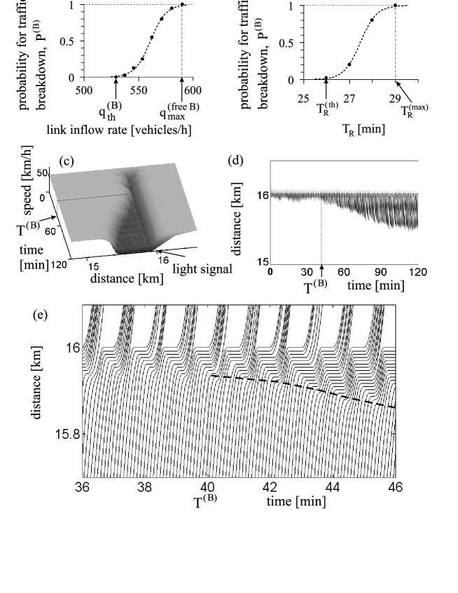
Figure 1: Spontaneous traffic breakdown at light signal of city link: Probability of traffic breakdown $P^{\rm(B)}$ as functions of inflow rate $q_{\rm in}$ into a single-lane link (a) and of duration of the red phase $T_{\rm R}$ (b). (c–e) Average speed in space and time (c) for simulation realization 1, the same data as that in (c) presented by regions with variable darkness (d) (the lower the speed, the darker the region; in white regions the speed is higher than 15 km/h), and vehicle trajectories (e) for a time interval related to (c, d). Cycle length of light signal is $\vartheta=T_{\rm G}+T_{\rm Y}+T_{\rm R}=$ 60 sec, duration of the yellow phase is $T_{\rm Y}=$ 2 sec, the observation time $T_{\rm ob}=$ 60 min Realization . In (b–e), $q_{\rm in}=$ 570 vehicles/h. In (a, c–e), duration of the red and green phases are $T_{\rm R}=$ 28 and $T_{\rm G}=$ 30 sec, respectively. Light signal is located at 16 km. Simulation model parameters, which are different from those presented in Table A2 of KKl2010 are: $v_{\rm free}=$ 55 km/h, $p_{a}=0.1$, $a^{(\rm a)}=a$, $v_{22}=7\ {\rm ms^{-1}}/\delta v$, $\Delta v_{22}=2\ {\rm ms^{-1}}/\delta v$, $v_{01}=6\ {\rm ms^{-1}}/\delta v$, $v_{21}=7\ {\rm ms^{-1}}/\delta v$, $a=$ 0.5 ${\rm ms^{-2}}/\delta a$, where $\delta v=$ 0.01 ${\rm ms^{-1}}$, $\delta a=$ 0.01 ${\rm ms^{-2}}$.

(iii) After the link inflow has been switched on, traffic breakdown occurs with a time delay $T^{\rm(B)}$ that can be considerably longer than cycle length $\vartheta$ of light signal. This means that at time $t<T^{\rm(B)}$ the queue developed during the red phase disolves fully during the green phase, i.e., the initial under-saturation regime of traffic exists at light signal. In particular, in Fig. 1 (c–e) we can see the under-saturation regime at light signal exists 39 cycles of light signal (39 minutes). However, at $t=T^{\rm(B)}=$ 40 min traffic breakdown occurs spontaneously (Fig. 1 (c–e)): The average outflow rate downstream of the link decreases from 570 to about 535 vehicles/h Flow and the under-saturation regime transforms into over-saturation. This occurs without any change in the link inflow rate $q_{\rm in}$ and light signal parameters. This traffic breakdown results in the non-reversible increase in the queue length at the light signal over time (Fig. 1(c, d)). The beginning of this non-reversible increase in the queue length at the light signal has been labeled by a dashed curve in Fig. 1(e).

(iv) The time delay $T^{\rm(B)}$ of traffic breakdown at light signal is a random value: In different simulation realizations (runs) made at the same given link inflow rate and parameters of light signal, we find very different values of $T^{\rm(B)}$. For example, in simulation realization 1 shown in Fig. 1 (c–e) as abovementioned $T^{\rm(B)}=$ 40 min, while in simulation realizations 2 shown in Fig. 2 (a, b) $T^{\rm(B)}=$ 20 min. In some of the realizations, no traffic breakdown occurs during 120 min (Fig. 2 (c, d)). This is associated with the result that traffic breakdown at light signal occurs within the flow rate range (3) with probability $0<P^{\rm(B)}<1$, i.e., in some realizations traffic breakdown occurs, whereas in other simulation realizations (runs) no traffic breakdown occurs at the same link inflow rate and light signal parameters.

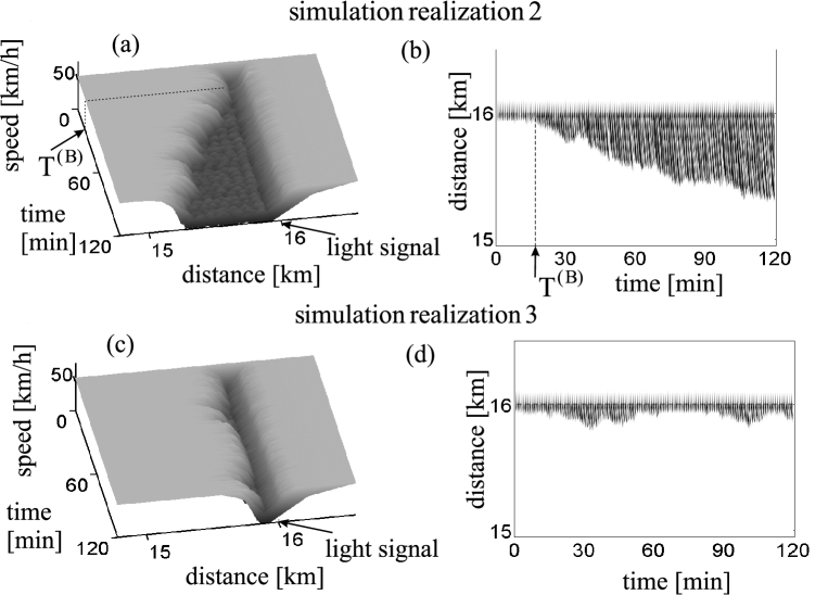
Figure 2: Two different simulation realizations (runs) calculated at the same model parameters as those used for the simulation realization 1 shown in Fig. 1 (c–e): (a, b) Traffic breakdown occurs after $T^{\rm(B)}=$ 20 min in realization 2. (c, d) No traffic breakdown occurs in realization 3.

(v) As expected, the non-reversible growth of the queue (Fig. 1 (c–e)) causes gridlock in a city. Indeed, while approaching an upstream city intersection, the queue prevents the free vehicle entering to the link from upstream city links leading to traffic breakdown at the upstream intersection (Fig. 3), and so on.

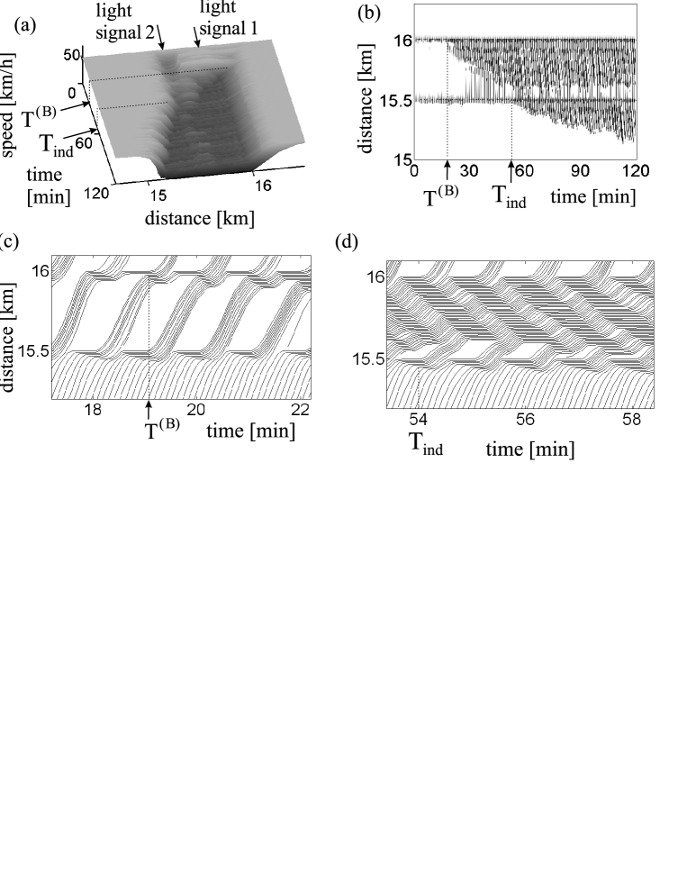
Figure 3: Traffic gridlock: (a, b) Speed in space and time (a) and the same data presented by regions with variable darkness (b). (c, d) Vehicle trajectories for two time intervals related to (a, b). Simulations of two network intersections: Link 1 with light signal 1 (at 16 km) at the downstream intersection is the same as that in Figs. 1 and 2; the inflow to link 1 consists of the outflows from links 2 and 3 for vehicles going to link 1 (inflow rates $q_{\rm in}=$ 545 and 36 vehicles/h for link 2 and 3, respectively) during the related green phases of respective light signals 2 and 3 (located at 15.5 km) at the upstream intersection. After time delay $T^{\rm(B)}=$ 19 min traffic breakdown occurs on link 1; the growing queue induces traffic breakdown on link 2 at $T_{\rm ind}=$ 54 min. $\vartheta=$ 60 sec, $T_{\rm Y}=$ 2 sec. $T_{\rm R}=$ 28 for links 1 and 2, 30 sec for link 3. Other model parameters are the same as those in Fig. 1.

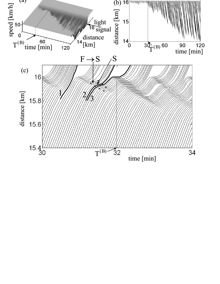
Figure 4: Physics of traffic breakdown: Speed in space and time (a) and the same data presented by regions with variable darkness (b) (in white regions the speed is higher than 25 km/h). (c) Vehicle trajectories related to (a, b). $q_{\rm in}=$ 1060 vehicles/h. $\vartheta=$ 60 sec, $T_{\rm Y}=$ 2 sec, $T_{\rm R}=$ 10 sec, $T_{\rm G}=$ 48 sec. Other parameters are the same as those in Fig. 1.

IV The physics of traffic breakdown at signalized city intersection

The physics of traffic breakdown at light signal is as follows:

1. At the end of the green phase in the under-saturation regime at light signal, there is at least one of the vehicles passing light signal without stopping (see vehicle trajectories for cycles of light signal at $t\leq$ 39 min, i.e., at $t<T^{\rm(B)}$ in Fig. 1(e)). Therefore, in the under-saturation regime the link outflow rate Flow is greater than after traffic breakdown has occurred leading to the over-saturation regime in which the vehicle queue length increases non-reversibly over time (Fig. 1 (c–e)).

2. Traffic breakdown at light signal is initiated by an F$\rightarrow$S transition upstream of the queue, as can be clearly seen if we consider a shorter duration of the red phase $T_{\rm R}=$ 10 sec (Fig. 4) at the same light signal cycle $\vartheta=$ 60 sec Real . Before traffic breakdown occurs, there are vehicles that pass light signal at the end of the green phase while moving at nearly maximum free flow speed $v_{\rm free}$ (vehicle trajectory 1 in Fig. 4 (c)). We find that just before traffic breakdown at $t=T^{\rm(B)}=$ 32 min occurs, an F$\rightarrow$S transition happens upstream of the queue developed at the previous cycle of light signal $t=T^{\rm(B)}-1=$ 31 min (labeled by arrow F$\rightarrow$S in Fig. 4 (c)). Due to the F$\rightarrow$S transition, synchronized flow at the end of the green phase is forming (region labeled by $S$ in Fig. 4 (c)). Thus rather than moving at a nearly free flow speed, at the end of the green phase vehicles begin to move at a lower synchronized flow speed (vehicle trajectory 2 in Fig. 4 (c)). As a result, these vehicles reach the location (16 km) of light signal later (vehicle 2) than they would do this while moving at nearly free flow speed (vehicle 1). Therefore, a smaller number of vehicles pass light signal during the green phase (19 and 12 vehicles for two subsequent green phases associated with vehicles 1 and 2, respectively). This explains why rather than pass light signal the following vehicle 3 in Fig. 4 (c) must stop during the next red phase. Thus the F$\rightarrow$S transition at the previous cycle of light signal results in traffic breakdown, i.e., in the emergence of the growing queue because due to a lower speed in synchronized flow the smaller number of vehicles pass light signal during the previous green phase.

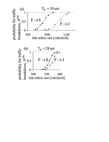
Figure 5: Comparison of the probability of traffic breakdown initiated by F$\rightarrow$S transition (curves labeled by F$\rightarrow$S) with the probability of traffic breakdown through a direct F$\rightarrow$J transition (curves labeled by F$\rightarrow$J) for $(T_{\rm R},\ T_{\rm G},\ T_{\rm Y})=$ (10, 48, 2) (a) and (28, 30, 2) (b) sec. $\vartheta=$ 60 sec. Curve labeled by F$\rightarrow$S in (b) is taken from Fig. 1 (a). A two-phase model used for simulations of F$\rightarrow$J transition follows from the Kerner-Klenov three-phase model after removing the description of driver behaviors associated with three-phase theory book – 2D-region of synchronized flow states and the associated speed adaptation effect within these states as well as the over-acceleration effect have been removed; this is done through the use of $G_{n}=0$ and $p_{a}=p_{1}=p_{2}=0$ in Table A1 of KKl2010 for the three-phase model. All characteristics of the F$\rightarrow$J transition and resulting wide moving jams in the three-phase and two-phase models are identical, in particular, the flow rate in free flow (at maximum speed 55 km/h) in the outflow from a wide moving jam is equal to $q_{\rm out}=$ 1614 vehicles/h. Other model parameters are the same as those in Fig. 1.

3. There is a great difference between highway traffic and traffic at light signal: In contrast with a highway bottleneck, light signal introduces always a very great non-homogeneity in traffic while forcing vehicles to stop during the red phase. However, there is a common feature of traffic breakdown at a highway bottleneck and at light signal. The probability of the emergence of a wide moving jam (J) at the highway bottleneck through a sequence of F$\rightarrow$S$\rightarrow$J transitions is greater than the probability of the jam formation in free flow (F$\rightarrow$J transition) book . Qualitatively the same result has been found in this article: Traffic breakdown at light signal, i.e., the growing queue formation initiated by an F$\rightarrow$S transition (Figs. 1–4) can be considered a sequence of F$\rightarrow$S$\rightarrow$J transitions (in contrast, the growing queue formation at light signal without an F$\rightarrow$S transition can be considered an F$\rightarrow$J transition). The probability of this sequence of F$\rightarrow$S$\rightarrow$J transitions at light signal is greater than the probability for the breakdown through an F$\rightarrow$J transition. To show this, we repeat the above simulations with a stochastic two-phase traffic model (see caption of Fig. 5). As in other two-phase models (see reviews Reviews ), in the two-phase model there is no a first-order F$\rightarrow$S transition and, therefore, traffic breakdown is caused by an F$\rightarrow$J transition. Simulations of the three-phase and two-phase models show that for main city links for which the green phase duration is not appreciably shorter than the red phase duration Equal , at any link inflow rate the probability for traffic breakdown initiated by the F$\rightarrow$S transition is considerably greater than for the F$\rightarrow$J transition (Fig. 5).

V Conclusions

We have found that in an initial under-saturated traffic controlled by light signal in which a vehicle queue developed during the red phase of light signal dissolves fully during the green phase, i.e., no traffic gridlock should be expected, nevertheless, traffic breakdown leading to city gridlock can occur with some probability after a random time delay. This traffic breakdown is initiated by an F$\rightarrow$S transition occurring upstream of the vehicle queue at light signal. The probability of traffic breakdown at light signal is an increasing function of the duration of the red phase of light signal and link inflow rate. A similar flow rate dependence of the breakdown probability has been found for a highway bottleneck book ; in this sense, light signal can be considered a bottleneck in a city network. Therefore, for the dynamic control of a city network that could be a very interesting task for future investigations the breakdown minimization (BM) principle can be applied BM ; Principle .

I thank S. Klenov and V. Friesen for discussions and S. Klenov for help in simulations.

References

- (1) N.H. Gartner, Ch. Stamatiadis, in Encyclopedia of Complexity and System Science, ed. by R.A. Meyers. (Springer, Berlin, 2009), pp. 9470-9500.
- (2) B.S. Kerner. The Physics of Traffic (Springer, Berlin, New York 2004); Introduction to Modern Traffic Flow Theory and Control (Springer, Berlin, New York 2009).
- (3) B.S. Kerner, S.L. Klenov, J. Phys. A: Theor. Math. 43 425101 (2010).
- (4) To find the probability of traffic breakdown , a study of traffic breakdown at light signal during a observation time is repeated for 40 different realizations for the same given link flow rates and light signal control parameters, however, at different initial conditions for random model fluctuations.
- (5) These functions can be approximated by formulae: , , where and depends on parameters of light signal control, whereas and depend on the link inflow rate and cycle length .
- (6) The link outflow rate is averaged during time that is considerably longer than cycle length of light signal.
- (7) This relation between green and red phases of light signal corresponds to a realistic case in which the link is related to a main road at a city intersection.
- (8) N.H. Gartner, C.J. Messer, A. Rathi (eds.). Traffic Flow Theory (Transportation Research Board, Washington, D.C. 2001); D.C. Gazis. Traffic Theory (Springer, Berlin 2002); D. Chowdhury, L. Santen, A. Schadschneider. Physics Reports 329, 199 (2000); D. Helbing. Rev. Mod. Phys. 73, 1067–1141 (2001); T. Nagatani. Rep. Prog. Phys. 65, 1331–1386 (2002); K. Nagel, P. Wagner, R. Woesler. Operation Res. 51, 681–716 (2003).
- (9) For 60 sec and 2 sec (Figs. 1–5), the probabilities for traffic breakdown through the FSJ and FJ transitions become to be identical only at 37 sec.
- (10) B.S. Kerner, J. Phys. A: Math. Theor. 44, 092001 (2011).
- (11) Indeed, in the case of city (or urban) networks the BM principle is as follows: The optimum of a traffic network with bottlenecks is reached, when dynamic traffic optimization and control are performed in the network in such a way that the probability for spontaneous occurrence of traffic breakdown in at least one of the network bottlenecks during a given observation time reaches the minimum possible value, i.e., the network optimum is reached at , where is the number of network links for which inflow rates can be adjusted, is the link inflow rate for a link with index ; , where ; is bottleneck index, ; is probability that during the time interval traffic breakdown occurs at bottleneck ; is the set of control parameters (e.g.,, control parameters of light signal) for one of these network bottlenecks with index (), . The BM principle is equivalent to , where is the probability that during time interval free flows remain in the network, i.e., that traffic breakdown occurs at none of the bottlenecks, .