The behavior of noise-resilient Boolean networks with diverse topologies

Abstract

The dynamics of noise-resilient Boolean networks with majority functions and diverse topologies is investigated. A wide class of possible topological configurations is parametrized as a stochastic blockmodel. For this class of networks, the dynamics always undergoes a phase transition from a non-ergodic regime, where a memory of its past states is preserved, to an ergodic regime, where no such memory exists and every microstate is equally probable. Both the average error on the network, as well as the critical value of noise where the transition occurs are investigated analytically, and compared to numerical simulations. The results for “partially dense” networks, comprised of relatively few, but dynamically important nodes, which have a number of inputs which greatly exceeds the average for the entire network, give very general upper bounds on the maximum resilience against noise attainable on globally sparse systems.

1 Introduction

An essential feature of many self-organized and artificial systems of several interacting elements is the ability of to function in a predictable fashion even in the presence of stochastic fluctuations, which are inherent to the system itself. Good examples are biochemical signaling networks and gene regulation in organisms [1], as well as artificial digital circuits, and communication networks [2]. In such systems, it is often the case that the source of the fluctuations cannot be entirely removed, and the system must be able to deal with them, by incorporating appropriate error-correction measures. These may include specific dynamical properties [3, 4], choice of functional elements and structural properties [5, 6], which one way or another result in enough information redundancy, which can be used to counteract the deviating effects of noise. In this work, the focus is turned on optimal bounds which can be attained by a wide class of such systems, when many parameters can be freely varied. More precisely, we consider a paradigmatic system of dynamically interacting Boolean elements, regulated by Boolean functions, where noise is introduced by the probability that at any time, any input of a given function can be “flipped” to its opposite value, before the output of the function is computed. The networks considered are regulated by optimal majority functions, and can possess arbitrary topological structures. The choice of majority functions corresponds to the limiting case where the trade-off between robustness against noise and fitness for a given task is at a maximum for every function in the network.

We obtain – both analytically and numerically – relevant properties of the system, such as the average probability of error as a function of noise, and critical value of noise, for which reliability is no longer possible. At this noise threshold, the system undergoes a dynamic phase transition from a non-ergodic regime, where a memory of its past states is preserved, to an ergodic regime, where no such memory exists and every microstate is equally probable. We identify the most relevant topological properties which can confer more robustness to the system, namely the existence of a more densely connected subset of the network, which is responsible for the dynamics of a significant portion of the system. The properties of such optimal topologies serve as general optimal bounds on the maximum resilience against noise which is attainable by this class of system.

The behavior of similar systems under noise has been studied previously by a number of authors. The dynamics of random Boolean networks (RBNs) with noise (random functions and topology, not necessarily aiming at robustness [7]) was studied in [8, 9, 10, 11, 12, 13, 14, 15]. The early works presented in [8, 9, 10] considered only small networks with $N\leq 20$ nodes, and focused on the average crossing time between trajectories in state space which started from different initial states. It was found that the trajectories must cross over “barriers,” which correspond to the attractor basin boundaries. However, the probability of crossing is always non-vanishing in such small systems. It was further shown in [15] that the dynamics of RBNs is always ergodic for any positive value of noise, and thus cannot preserve any memory of its past states. However, this is not true for random networks composed of threshold or majority functions, as shown in [11, 16]. These networks undergo the aforementioned phase transition between ergodicity and non-ergodicity at a critical value of noise. The same type of transition has also been observed for Boolean systems composed of majority functions, but having acyclic and stratified topology (i.e. Boolean formulas) [17, 18]. It was also shown in [5] that this transition has a general character, since any Boolean network can be made robust by introducing an appropriate restoration mechanism with majority functions.

Boolean networks with majority functions share some similarities with the so-called majority voter model [19, 20], which is usually defined on undirected regular lattices. This system also undergoes a phase-transition based on noise, which belongs to the universality class of the Ising model [21].

The issue of reliable computation under noise has also been tackled by the mathematical community, starting with von Neumann [22], who was the first to notice an important difference between reliable computation of noisy Boolean circuits and the more general scenario of reliable communication considered by Shannon [2], namely that it is not possible to guarantee an arbitrarily small error rate, if the a given circuit has a fixed number of inputs per function. He also pointed out that reliable computation is not at all possible for Boolean functions with three inputs after a given noise threshold. His results were later improved by Evans and Pippinger [23], who proved a similar bound for Boolean formulas with two inputs per node, and finally Evans and Schulman [24] who proved the bound for Boolean formulas with any odd number of inputs per node. Recently, an extension to these bounds which are also valid for functions with even number of inputs was derived in [25].

This paper is divided as follows. In section 2 we describe the model and in section 3 we analyse the phase transition based on noise for several different topological models: In 3.1 we consider random networks with a single-valued in-degree distribution, and in 3.2 we extend the model to arbitrary in-degree distributions. In 3.3 we consider a more general stochastic blockmodel, which represents a much larger class of possible topological structures. We finalize in section 4 with some concluding remarks.

2 The model

A Boolean Network (BN) [26, 27] is a directed graph of $N$ nodes representing Boolean variables $\mathbf{\sigma}\in\{1,0\}^{N}$, which are subject to a deterministic update rule,

$$\sigma_{i}(t+1)=f_{i}\left(\bm{\sigma}(t)\right)$$ (1)

where $f_{i}$ is the update function assigned to node $i$, which depends exclusively on the states of its inputs. It is also considered that all nodes are updated in parallel.

Here, noise is included in the model by introducing a probability $P$ that at each time-step a given input has its value “flipped”: $\sigma_{j}\to 1-\sigma_{j}$, before the output is computed [15]. This probability is independent for all inputs in the network, and many values may be flipped simultaneously. The functions on all nodes are taken to be the majority function, defined as

$$f_{i}(\{\sigma_{j}\})=\begin{cases}1\text{ if }\sum_{j}\sigma_{j}>k_{i}/2,\\ 0\text{ otherwise, }\end{cases}$$ (2)

where $k_{i}$ is the number of inputs of node $i$. The definition above will lead to a bias if $k_{i}$ is an even number, since if the sum happens to be exactly $k_{i}/2$ the output will be $0$, arbitrarily. Alternative definitions could be used, which would remove the bias [28]. Instead, for the sake of simplicity, in this work all values of $k_{i}$ considered will be odd, making this bias a non-issue.

Starting from a given initial configuration, the dynamics of the system evolves and eventually reaches a dynamically stable regime, where (for sufficiently large systems) the average value $b_{t}$ of $1$’s no longer changes, except for stochastic fluctuations [11]. In the absence of noise ($P=0$) there are only two possible attractors (if the network is sufficiently random and not disjoint), where all nodes have the same value, which can be either $0$ or $1$. We will consider these homogeneous attractors as being the “correct” dynamics, and denote the deviations from them as “errors”. More specifically, without loss of generality, we will name the value of $1$ as an “error”, and the value of $b_{t}$ as the average error on the system.

We note that the above model has an optimal character regarding robustness against noise, for the following two reasons: 1. It is known that the majority function as defined in Eq. 2 is optimal in the case of fully redundant inputs (i.e. in the absence of noise, they all have simultaneously the same value), which have an uniform and independent probability of being “flipped” by noise. In this situation, the output of the majority function will be “correct” with greater probability than any other function with the same number of inputs [22, 24]. 2. The existence of only two possible attractors with uniform values can be interpreted as an extremal trade-off between dynamical function and increased resilience against noise: A network with more elaborate dynamics in the absence of noise, composed of many attractors with smaller basis of attraction, would be invariably more difficult to stabilize if noise is present, since it would become harder to distinguish between dynamical states.

3 Dynamical phase transition based on noise

As previously defined, the average “error” on the network is characterized by the average value of $1$’s in the network at a given time, $b_{t}$. In this section we will obtain the value of $b_{t}$ for networks with different topological characteristics. We will focus first on uniform random networks with all functions having the same in-degree, and networks with arbitrary in-degree distributions. We then move to an arbitrary blockmodel, which can incorporate more general topological features.

3.1 Single-valued in-degree distribution

In this session, we compute the value of $b_{t}$ for networks composed of nodes with the same number $k$ of inputs per node, which are randomly chosen between all possible nodes. This type of system has been studied before by Huepe et al [11] and is essentially equivalent to the same problem posed for Boolean formulas by Evans et. al [24], since the presence of short loops can be neglected for large networks. For the sake of clarity, we shortly reproduce the analysis developed in [24], and we extend it by calculating the critical exponent of the transition. We then proceed to generalize the approach to more general topologies in the subsequent sections.

In order to obtain an equation for the time evolution of $b_{t}$ we employ the usual annealed approximation [29], which assumes that at each time step the inputs of every function are randomly re-sampled, such that any quenched topological correlations are ignored, and all inputs will have the same probability $b_{t}$ of being equal to $1$. If the inputs of a majority function have a value of $1$ with probability $b$ (independently for each input), the output will also be $1$ with a probability given by

$$m_{k}(b)=\sum_{i={\lceil k/2\rceil}}^{k}{k\choose i}b^{i}(1-b)^{k-i}.$$ (3)

The time evolution of $b_{t}$ can then be written as

$$b_{t+1}=m_{k}\left((1-2P)b_{t}+P\right),$$ (4)

where $P$ is the noise probability, as described previously. The right-hand side of Eq. 4 is symmetric in respect to values of $b_{t}$ around $1/2$ (as can be seen in Fig. 1), such that the dynamics for values of $b^{\prime}_{t}>1/2$, can be obtained from $b^{\prime}_{t}=1-b_{t}$, with $b_{t}<1/2$. Thus, without loss of generality, we will only consider the case $b_{t}\leq 1/2$ throughout the paper.

Given any initial starting value $b_{0}\leq 1/2$, the dynamics will always lead to a fixed point $b^{*}\leq 1/2$, which is a solution of Eq. 4, with $b_{t+1}=b_{t}\equiv b^{*}$. This is in general a solution of a polynomial of order $k$, for which there are no general closed-form expression. However, since the right-hand side of Eq. 4 is a monotonically increasing function on $b_{t}$, we can conclude there can be at most two possible fixed points: $b^{*}=1/2$ (ergodic regime) or $b^{*}<1/2$ (non-ergodic regime). Furthermore, considering the right-hand side of Eq. 4 is a convex function (for $b_{t}\leq 1/2$, as is always assumed), if the fixed point $b^{*}=1/2$ becomes stable, i.e. $\frac{db_{t+1}}{db_{t}}|_{b^{*}=1/2}\leq 1$, the other fixed point $b^{*}<1/2$ must cease to exist, since in this case $b_{t+1}>b_{t}$ for any $b_{t}<1/2$. Thus, the value of $P$ for which $b^{*}=1/2$ becomes a stable fixed point marks the transition from non-ergodicity to ergodicity. In order to obtain this value, we need to compute the the derivative of the right-hand side of Eq. 4 in respect to $b_{t}$. Using the derivative of Eq. 3 (see  [24] for a detailed derivation of this expression),

$$m^{\prime}_{k}(b)\equiv\frac{dm_{k}(b)}{db}=\frac{k}{2^{k-1}}{k-1\choose{\lfloor k/2\rfloor}}[1-(1-2b)^{2}]^{{\lfloor k/2\rfloor}}$$ (5)

we have that $(1-2P^{*})m^{\prime}_{k}(1/2)=1$, where $P^{*}$ is the critical value of noise. Thus, a full expression for $P^{*}$ is given by

$$P^{*}=\frac{1}{2}-\frac{2^{k-2}}{k{k-1\choose{\lfloor k/2\rfloor}}}.$$ (6)

Taking the limit $k\gg 1$, one obtains $P^{*}\approx\frac{1}{2}-\frac{1}{2}\sqrt{\frac{\pi}{2k}}$ using the Stirling approximation. Eq. 6 is the main result of [24]. We note however that a slightly less explicit but more general expression was derived previously in [11], for the case where the majority function accepts inputs with different weights.

For a given value of $k$, the value of $b^{*}$ increases continuously with $P$ until it reaches $1/2$ for $P\geq P^{*}$ (see Fig. 1), characterizing a second-order phase transition. One can go further and obtain the critical exponent of the transition by expanding Eq. 3 near $b=1/2$,

$$m_{k}(b)=\frac{1}{2}-\frac{1}{2}m^{\prime}_{k}(1/2)(1-2b)+\frac{1}{6}{\lfloor k/2\rfloor}m^{\prime}_{k}(1/2)(1-2b)^{3}+O\left((1-2b)^{5}\right)$$ (7)

and using it in 4, and solving for $b^{*}=b_{t+1}=b_{t}$, which leads to

$$b^{*}\approx\frac{1}{2}-\left[\frac{3}{2}\frac{m^{\prime}_{k}(1/2)^{3}}{{\lfloor k/2\rfloor}}\widetilde{P}\right]^{1/2}$$ (8)

where $\widetilde{P}=P^{*}-P$. From this expression it can be seen that the critical exponent is $1/2$, corresponding to the mean-field universality class.

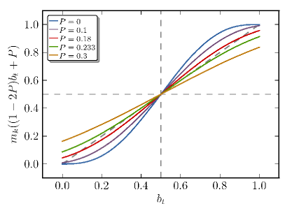
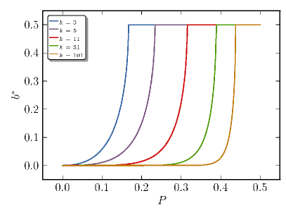
Figure 1: The dynamic map of Eq. 4 for different values of $P$ (left), and the value of the stable fixed-point $b^{*}\leq 1/2$, as a function of $P$ (right).

The values of $b^{*}$ and $P^{*}$ can be understood as general bounds on the minimum error level and maximum tolerable noise, respectively, which must hold for random networks composed of functions with the same number of inputs. These are rather stringent conditions, and it is possible to imagine interesting situations where they are not fulfilled. Therefore, for more general bounds, one needs to relax these restrictions. We proceed in this direction in the following section, where we consider the case of arbitrary in-degree distributions, but otherwise random connections among the nodes.

3.2 Arbitrary in-degree distributions

We turn now to uncorrelated random networks with an arbitrary distribution of inputs per node (in-degree), $p_{k}$. Here it is assumed that the inputs of each function are randomly chosen among all possibilities, and that the in-degree distribution $p_{k}$ provides a complete description of the network ensemble. This configuration was also considered in [16], for a more general case where the inputs can have arbitrary weights. We analyse here the special case with no weights in more detail, and obtain more explicit results.

The annealed approximation can be used in the same manner as in the previous section: One considers simply that at each time step the inputs of each function are randomly chosen . The time evolution of $b_{t}$ now becomes,

$$b_{t+1}=\sum_{k}p_{k}m_{k}\left((1-2P)b_{t}+P\right).$$ (9)

Like for Eq. 4, there are only two fixed points $b^{*}\leq 1/2$, and the transition can be obtained by analysing the stability of the fixed point $b^{*}=1/2$. In an entirely analogous fashion to Eq. 6, using the derivative of the right-hand side of Eq. 9 one obtains the following expression for the critical value of noise,

$$P^{*}=\frac{1}{2}-\left[\sum_{k}p_{k}\frac{k{k-1\choose{\lfloor k/2\rfloor}}}{2^{k-2}}\right]^{-1}.$$ (10)

Considering the limit where all $k\gg 1$, one has $P^{*}\approx\frac{1}{2}-\left[\sqrt{\frac{8}{\pi}}\sum_{k}p_{k}\sqrt{k}\right]^{-1}$. Note that the above expression only holds if $p_{k}=0$ for every $k$ which is even, as is assumed throughout the paper. The critical exponent can also be calculated in an analogous fashion, and is always $1/2$, unless $p_{k}$ has diverging moments. In this case the critical exponents will depend on the details of the distribution (see [16] for a more thorough analysis).

With this result in mind, one can ask the following question: What is the best in-degree distribution, for a given average in-degree ${\left<k\right>}$, such that either $b_{t}$ is minimized or $P^{*}$ is maximized? As it will now be shown, in either case the best distribution is the single-valued distribution, already considered in the previous section. For simplicity, let us consider the case where ${\left<k\right>}$ is discrete and odd. We begin with the analysis of $b_{t}$. We can observe that for $b\leq 1/2$, $m_{k}(b)$ is a convex function on $k$ (see Fig 2),

$$m_{k}(b)\leq\frac{m_{k-2}(b)+m_{k+2}(b)}{2},$$ (11)

and thus by Jensen’s inequality we have that $m_{{\left<k\right>}}(b)\leq{\left<m_{k}(b)\right>}$. Since the equality only holds only for the single-valued distribution $p_{k}=\delta_{k,{\left<k\right>}}$ (assuming $b\notin\{0,1/2\}$), the right-hand side of Eq. 9 will always be larger for any other distribution $p_{k}$. The same argument can be made for the value of $P^{*}$: Since we have that $(1-2P^{*})^{-1}=\sum_{k}p_{k}m^{\prime}_{k}(1/2)$, and $m^{\prime}_{k}(1/2)$ is a concave function on $k$,

$$\frac{m^{\prime}_{k-2}(1/2)+m^{\prime}_{k+2}(1/2)}{2} =\frac{m^{\prime}_{k}(1/2)}{2}\left[\frac{k-1}{k}+\frac{k+2}{k+1}\right]$$ (12)

$$=m^{\prime}_{k}(1/2)\left[1-\frac{1}{2k(k+1)}\right]$$ (13)

$$<m^{\prime}_{k}(1/2)$$ (14)

we have that $m^{\prime}_{{\left<k\right>}}(1/2)\geq{\left<m^{\prime}_{k}(1/2)\right>}$. Again, the equality only holds only for $p_{k}=\delta_{k,{\left<k\right>}}$, which is therefore the optimal scenario.

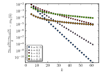
Figure 2: Convexity of $m_{k}(b)$, as stated in Eq. 11.

One special case which merits attention is the scale-free in-degree distribution

$$p_{k}\propto k^{-\gamma},$$ (15)

which occurs often in many systems, including, as some suggest, gene regulation [30]. It is often postulated that networks with such a degree distribution are associated with different types of robustness, due to their lower percolation threshold [31] which can be interpreted as a resilience to node removal “attacks”. However, in the case of robustness against noise Eq. 15 by itself does not confer any advantage. For instance, from Eq. 10, using Stirling’s approximation one sees that the expression within brackets will diverge only if $\gamma\leq 3/2$, leading to $P^{*}=1/2$. This means that for $3/2<\gamma\leq 2$, we have that the average in-degree diverges (${\left<k\right>}\to\infty$) but the critical value of noise is still below $1/2$. This is considerably worse, for instance, than a fully random network with in-degree distribution given by a slightly modified Poisson, which is defined only over odd values of $k$,

$$p_{k}=\frac{1}{\sinh\lambda}\frac{\lambda^{k}}{k!},$$ (16)

with ${\left<k\right>}=\lambda/\tanh\lambda$. For this distribution, we have that $P^{*}\to 1/2$ for ${\left<k\right>}\to\infty$, as one would expect also for the single-valued distribution. A comparison between these two distributions is shown in Fig. 3.

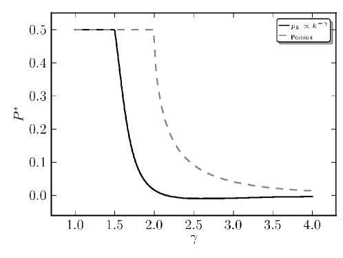
Figure 3: Critical value of noise $P^{*}$ as a function of $\gamma$ for the scale-free in-degree distribution given by Eq. 15 and for the Poisson distribution given by Eq. 16, where $\lambda$ is chosen such that the average in-degree is the same for both distributions.

The above analysis shows that the single-valued in-degree distribution $p_{k}=\delta_{k,{\left<k\right>}}$ is the best one can hope for with a given average in-degree ${\left<k\right>}$, as long as the inputs of each function are randomly chosen. However, this is a restriction which does not need be fulfilled in general. In order to obtain more general bounds, one needs to depart from this restriction, and consider more heterogeneous possibilities, which is the topic of the next section.

3.3 Arbitrary topology: Stochastic blockmodels

We now consider a much more general class of networks known as stochastic blockmodels [32, 33, 34], where it is assumed that every node in the network can belong one of $n$ distinct classes or “blocks”. Every node belonging to the same block has on average the same characteristics, such that we need only to describe the degrees of freedom associated with the individual blocks. In particular we use the degree-corrected variant [35] of the traditional stochastic blockmodel, which incorporates degree variability inside the same block. Here, we define $w_{i}$ to be the fraction of the nodes in the network which belong to block $i$, and $p^{i}_{k}$ is the in-degree distribution of block $i$. The matrix $w_{j\to i}$ describes the fraction of the inputs of block $i$ which belong to block $j$. We have therefore that $\sum_{i}w_{i}=1$, $\sum_{j}w_{j\to i}=1$ and $\sum_{i,k}kw_{i}p^{i}_{k}={\left<k\right>}$. Since the out-degrees are not explicitly required to describe the dynamics, they will be assumed to be randomly distributed, subject only to the restrictions imposed by $w_{i}$ and $w_{j\to i}$.

In the limit where the number of vertices $Nw_{i}$ belonging to each blocks $i$ is arbitrary large, we can use a modified version of the annealed approximation to describe the dynamics: Instead of randomly re-assigning inputs for each function, we choose randomly only amongst those which do not invalidate the desired block structure. In other words, we impose that after each random input rewiring, the inter-block connections probabilities are always given by $w_{j\to i}$. In this way, we maintain the dynamic correlations associated with the block structure, and remove those arising from quenched topological correlations present in a single realization of the blockmodel ensemble. Due to the self-averaging properties of this ensemble, for sufficiently large networks the annealed approximation is expected to be exact, in the same way it is for random networks without block structures.

With this ansatz, we can write the average value of $b_{i}$ for each block over time as

$$b_{i}(t+1)=\sum_{k}p_{k}^{i}m_{k}\left((1-2P)\sum_{j}w_{j\to i}b_{j}(t)+P\right),$$ (17)

which is a system of $n$ coupled maps. It is easy to see that $b^{*}_{i}=1/2$ is a fixed point of Eq. 17. In order to perform the stability analysis we have to consider the Jacobian matrix of the right-hand side of Eq. 17,

$$J_{ij}=\frac{\partial b_{i}(t+1)}{\partial b_{j}(t)}=(1-2P)w_{j\to i}\sum_{k}p^{i}_{k}m^{\prime}_{k}\left((1-2P)\sum_{j}w_{j\to i}b_{j}(t)\right).$$ (18)

At the fixed-point $b_{i}(t)=1/2$ we can write the Jacobian as

$$\bm{J^{*}}=(1-2P)\bm{M},$$ (19)

where matrix $\bm{M}$ is given by

$$M_{ij}=w_{j\to i}\sum_{k}p^{i}_{k}m^{\prime}_{k}(1/2).$$ (20)

The largest eigenvalues of $\bm{J^{*}}$ and $\bm{M}$, $\lambda$ and $\xi$ respectively, are related to each other simply by $\lambda=(1-2P)\xi$. Since the fixed-point in question will cease to be stable for $\lambda=1$, we have that the critical value of noise is given by

$$P^{*}=\frac{1}{2}-\frac{1}{2\xi}.$$ (21)

Thus, for $P>P^{*}$ the fixed point $b_{i}(t)=1/2$ becomes a stable fixed-point, and this marks the transition from non-ergodicity to ergodicity, as in the previous cases.

We note that the sizes of the blocks $w_{i}$ play no role in Eq. 21, and only the correlation probabilities $w_{i\to j}$ and the in-degree distributions $p^{i}_{k}$ define the value of $P^{*}$. For this reason, the average error $b^{*}=\sum_{i}w_{i}b_{i}$ on the network may not be always a suitable order parameter to identify the aforementioned phase transition, since the blocks which are responsible for the value of $P^{*}$ may be arbitrarily small in comparison to the rest of the network. However, these are obviously corner cases, since the most interesting situations are those where all blocks are relevant to the dynamics (or a given block could be otherwise ignored).

Given any desired many-block structure, one could find the largest eigenvalue $\xi$ of the matrix $\bm{M}$ and then determine the critical value of noise with Eq. 21. In the following, we will focus on the simplest nontrivial block structure which is composed only of two blocks. Such 2-block systems are fully accessible analytically, and are sufficient to obtain more general upper and lower bounds on the values of $P^{*}$ and $b^{*}$, respectively.

3.4 2-block structures

Here we consider networks composed of two blocks, where the block with the largest average in-degree will be labeled “core”. The size and average in-degree of the core block are $w_{c}$ and $k_{c}$ respectively, and for the non-core block $w_{r}=1-w_{c}$ and $k_{r}=({\left<k\right>}-w_{c}k_{c})/(1-w_{c})$. For simplicity, we will consider that the in-degree distribution of each block is the single-valued distribution $p^{i}_{k}=\delta_{k,k_{i}}$, where $k_{i}$ is the average in-degree of the block.

The matrix $w_{j\to i}$ has the general form

$$\bm{w_{\to}}=\left(\begin{array}[]{cc}w_{c\to c}&w_{c\to r}\\ w_{r\to c}&w_{r\to r}\end{array}\right)=\left(\begin{array}[]{cc}m_{c}&m_{r}\\ 1-m_{c}&1-m_{r}\end{array}\right),$$ (22)

with only two free variables $m_{c}$ and $m_{r}$, denoting the fraction of inputs which belong to the core block, for both blocks. Instead of considering all possible values of $m_{c}$ and $m_{r}$, we consider the following parametrization

$$m_{c} =\begin{cases}4a(1-a)w_{c}&\text{if }a\leq 1/2\\ m_{r}&\text{if }a>1/2\end{cases}$$ (23)

$$m_{r} =1-4a(1-a)(1-w_{c}),$$

where the single parameter $a\in[0,1]$ allows for the topology to be continuously varied between three distinct topological configurations (see Fig. 4): For $a=0$ we have a “restoration” topology, where the network is bipartite, and all inputs from the non-core block belong to the core block and vice-versa; for $a=1/2$ the inputs are randomly selected; and for $a=1$ we have a “segregated core” structure, where all the inputs of both blocks belong exclusively to the core block.

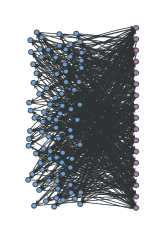
$a=0$

Restoration

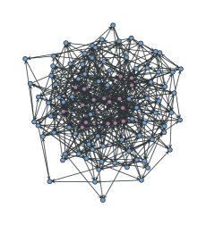
$a=1/2$

Random

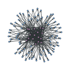
$a=1$

Segregated core

Figure 4: Three distinct 2-block structures possible with the parametrization given by Eq. 23, for different values of the parameter $a$.

For this system we can write the matrix $\bm{M}$ from Eq. 20 as

$$\bm{M}=\left(\begin{array}[]{cc}w_{c\to c}m^{\prime}_{k_{c}}(1/2)&w_{r\to c}m^{\prime}_{k_{c}}(1/2)\\ w_{c\to r}m^{\prime}_{k_{r}}(1/2)&w_{r\to r}m^{\prime}_{k_{r}}(1/2)\end{array}\right),$$ (24)

from which we can extract the largest eigenvalue $\xi$,

$$\xi=\frac{1}{2}(w_{c\to c}m^{\prime}_{k_{c}}(1/2)+w_{r\to r}m^{\prime}_{k_{r}}(1/2))\quad+\\ \frac{1}{2}\sqrt{4w_{r\to c}w_{c\to r}m^{\prime}_{k_{c}}(1/2)m^{\prime}_{k_{r}}(1/2)+\left(w_{c\to c}m^{\prime}_{k_{c}}(1/2)-w_{r\to r}m^{\prime}_{k_{r}}(1/2)\right)^{2}}.$$ (25)

From $\xi$, the critical value of noise can be obtained by Eq. 21.

The general behaviour of the asymptotic average error $b^{*}\equiv\lim_{t\to\infty}{\left<b_{i}(t)\right>}$, computed from Eq. 17 as a function of $a$ is shown in Fig. 5 for ${\left<k\right>}=5$ and $k_{r}=3$, and several values of $k_{c}$ (and $w_{c}$ chosen accordingly). In the same figure are shown results from numerical simulations of quenched networks with $N=10^{5}$ nodes, evolved according to Eq. 1, showing perfect agreement. On the right of Fig. 5 are shown the values of $b^{*}$ according to the reduced noise $P-P^{*}$, with $P^{*}$ computed according to Eqs. 25 and 21. The calculated values of $P^{*}$ for several values of $k_{c}$ are plotted on the right of Fig. 6. The nature of the phase transition is systematically the same, as can be seen in the right of Fig. 6, where the slope of the curves correspond to mean-field critical exponent $1/2$.

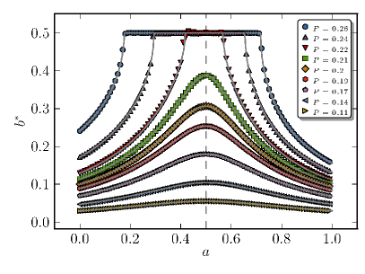
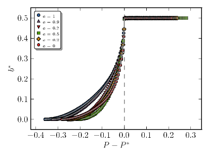
Figure 5: Average error $b^{*}$ as a function of $a$ for different values of noise $P$ (left) and as a function of the reduced noise $P-P^{*}$, with $P^{*}$ computed according to Eqs. 25 and 21, for several values of $a$ (right). All curves are for ${\left<k\right>}=5$, $k_{r}=3$ and $k_{c}=19$. The symbols are results of numerical simulations of quenched networks with $N=10^{5}$ nodes, and the solid lines are numerical solutions of Eq. 17.

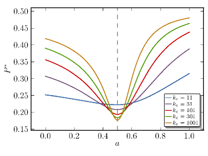
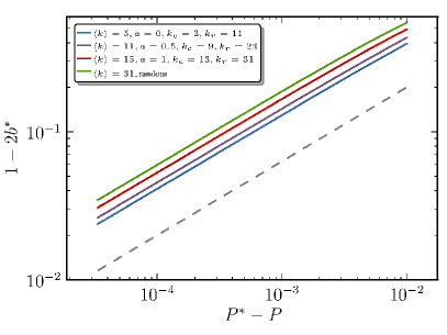
Figure 6: Critical value of noise $P^{*}$ as a function of $a$, for several values of $k_{c}$, with $k_{r}=3$ and ${\left<k\right>}=5$ (left), and value of $1-2b^{*}$ as a function of $P-P^{*}$ close to the critical point, for different values of ${\left<k\right>}$, $a$, $k_{r}$ and $k_{c}$ (right). The dashed line corresponds to a function proportional to $(P-P^{*})^{1/2}$.

It is interesting to compare the performance of the restoration ($a=0$) and segregated core ($a=1$) topologies. Both outperform the random topology ($a=1/2$), but the segregated core is always the best possible, having both the lowest values of $b^{*}$ and largest values of $P^{*}$. This is not surprising, since the segregated core is nothing more than an isolated network, which is more densely connected than the whole network, to which the remaining nodes are enslaved. On the other hand it is rather interesting how the restoration topology ($a=1$) is only marginally worse than the segregated core, since in this situation every node is dynamically relevant. We note that the relative advantage of the partially random topologies ($0<a<1$) may depend on the actual value of noise. This can be seen in Fig. 5 (right), where the curves for $b^{*}$ with different values of $a$ cross each other when $P-P^{*}$ is varied (the same is also observed when the curves are plotted against $P$). The reason for this is that the relative advantage of the segregated core topology in respect to restoration may manifest itself only as the value of noise approaches the critical point. For lower values of noise it is possible, for instance, for a full restoration topology with $a=0$ to outperform a partial segregated core structure with $a=0.9$, since it will perform comparably to a full segregation, $a=1$ (see Fig. 5, left). However, as noise is increased the relative advantage of the segregated topology makes up for this difference. In the general case, therefore, the optimal topology will depend on the value of noise.

Either with the restoration and segregated core topologies, the values of $b^{*}$ and $P^{*}$ become increasingly better for larger values of $k_{c}$, as can be seen in Figs. 6 and 7. One can therefore postulate that an optimum bound can be achieved for $k_{c}\to\infty$. Let us consider the situation where $w_{c}\propto 1/k_{c}$, such that $\lim_{k_{c}\to\infty}{\left<k\right>}=k_{r}$. For both $a=0$ and $a=1$ the value of $b^{*}$ approaches asymptotically $m_{{\left<k\right>}}(P)$, for $k_{c}\to\infty$, as can be seen in Fig. 7. This means that the average error of the core nodes will eventually vanish, and the remaining nodes will encounter the optimal scenario where the inputs are affected by the noise $P$ alone, and the error does not accumulate over time. It is therefore safe to conclude that

$$b_{\text{min}}=m_{{\left<k\right>}}(P)$$ (26)

is a general lower bound on the average error on a network with average in-degree ${\left<k\right>}$ and an arbitrary topology, which is asymptotically achieved for both the restoration and segregation topologies, for $k_{c}\to\infty$.

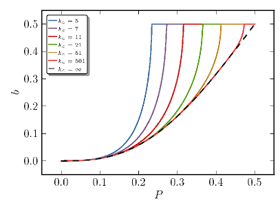
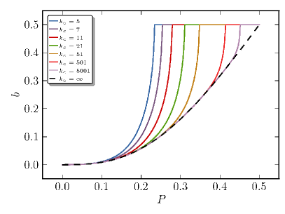
Figure 7: Values of $b^{*}$ as a function of $P$ for 2-block structures with $a=1$ (left) and $a=0$ (right), with $w_{c}=1/(100\times k_{c})$, $k_{r}=5$ and several values of $k_{c}$. The dashed curves are given by Eq. 26 with ${\left<k\right>}=k_{r}$.

4 Conclusion

We have investigated the behaviour of optimal Boolean networks with majority functions and different topologies in the presence of stochastic fluctuations. The dynamics of these networks undergo a phase transition from ergodicity to non-ergodicity. The non-ergodic regime can be can be interpreted as robustness against noise, since there is a permanent global memory of the initial condition. The ergodic phase, on the other hand, represents a situation where the effect of noise has destroyed any possible long-term dynamical organization of the system. We obtained, both analytically and numerically, the average error and the critical value of noise for networks composed of arbitrary in-degree distributions and for a more general stochastic blockmodel, which can accommodate a wide variety of network structures. We showed that both the average error level as well as the critical value of noise are improved both for the segregated core and restoration topologies, where the dynamics is dominated by a smaller subset of nodes, which have an above-average in-degree. In the limit where the average in-degree of these “core” nodes diverges, the network achieves an optimum bound, which corresponds to the maximum resilience attainable.

In a separate work [6], we show that segregated core structures emerge naturally out of an evolutionary process which favors robustness against noise.

As was discussed, the networks considered are made from optimal elements, which in isolation have the best possible behaviour. Because of this, the results obtained have a general character, and show the best scenario which can in general be achieved, under the constraints considered. However, it is important to point out that there are different types of stochastic fluctuations which can be considered in Boolean systems. Other than the type of noise considered in this work, it is possible for instance to incorporate fluctuations in the update schedule of the nodes [36]. It has been shown in [37], for random networks, that even if the update schedule is completely random, ergodicity is preserved, and the dynamics eventually leads to distinct attractors. Furthermore, it was shown in [3] that it is possible to obtain absolute resilience against noise in the update sequence, where the trajectories are always the same, independent of the update schedule used. In [4] this type of resilience has been coupled with single-flip perturbations, which correspond to very small values of the noise parameter $P$ considered in this work, and it was shown that arbitrary mutual resilience is also possible. The broader question of how a single system can be simultaneously robust against many different types of perturbations, and which features become more important in this case, still needs to be systematically tackled.

References

References

- [1] H. Kitano, “Biological robustness,” Nat Rev Genet, vol. 5, pp. 826–837, Nov. 2004.
- [2] C. E. Shannon, “A mathematical theory of communication,” Bell Syst Tech. J, vol. 27, no. 379, p. 623, 1948.
- [3] T. P. Peixoto and B. Drossel, “Boolean networks with reliable dynamics,” Physical Review E, vol. 80, p. 056102, Nov. 2009.
- [4] C. Schmal, T. P. Peixoto, and B. Drossel, “Boolean networks with robust and reliable trajectories,” New Journal of Physics, vol. 12, p. 113054, Nov. 2010.
- [5] T. P. Peixoto, “Redundancy and error resilience in boolean networks,” Physical Review Letters, vol. 104, p. 048701, Jan. 2010.
- [6] T. P. Peixoto, “Emergence of robustness against noise: A structural phase transition in evolved models of gene regulatory networks,” 1108.4341, Aug. 2011.
- [7] B. Drossel, “Random boolean networks,” Reviews of Nonlinear Dynamics and Complexity: Volume 1, 2008.
- [8] E. N. Miranda and N. Parga, “Noise effects in the kauffman model,” Europhys. Lett., vol. 10, pp. 293–298, 1989.
- [9] O. Golinelli and B. Derrida, “Barrier heights in the kauffman model,” J. Phys, vol. 50, pp. 1587–1601, 1989.
- [10] X. Qu, M. Aldana, and L. P. Kadanoff, “Numerical and theoretical studies of noise effects in the kauffman model,” Journal of Statistical Physics, vol. 109, no. 5, p. 967–986, 2002.
- [11] C. Huepe and M. Aldana-González, “Dynamical phase transition in a neural network model with noise: An exact solution,” Journal of Statistical Physics, vol. 108, no. 3, pp. 527–540, 2002.
- [12] A. Aleksiejuk, J. A. Holyst, and D. Stauffer, “Ferromagnetic phase transition in Barabási-Albert networks,” Physica A: Statistical Mechanics and its Applications, vol. 310, pp. 260–266, July 2002.
- [13] J. O. Indekeu, “Special attention network,” Physica A, vol. 333, pp. 461–464, Feb. 2004.
- [14] C. Fretter, A. Szejka, and B. Drossel, “Perturbation propagation in random and evolved boolean networks,” New Journal of Physics, vol. 11, no. 3, p. 033005, 2009.
- [15] T. P. Peixoto and B. Drossel, “Noise in random boolean networks,” Physical Review E, vol. 79, p. 036108, Mar. 2009.
- [16] M. Aldana and H. Larralde, “Phase transitions in scale-free neural networks: Departure from the standard mean-field universality class,” Physical Review E, vol. 70, p. 066130, Dec. 2004.
- [17] A. Mozeika, D. Saad, and J. Raymond, “Computing with noise: Phase transitions in boolean formulas,” Physical Review Letters, vol. 103, p. 248701, Dec. 2009.
- [18] A. Mozeika, D. Saad, and J. Raymond, “Noisy random boolean formulae: A statistical physics perspective,” Physical Review E, vol. 82, p. 041112, Oct. 2010.
- [19] M. J. Oliveira, “Isotropic majority-vote model on a square lattice,” Journal of Statistical Physics, vol. 66, pp. 273–281, Jan. 1992.
- [20] M. J. d. Oliveira, J. F. F. Mendes, and M. A. Santos, “Nonequilibrium spin models with ising universal behaviour,” Journal of Physics A: Mathematical and General, vol. 26, pp. 2317–2324, May 1993.
- [21] G. Grinstein, C. Jayaprakash, and Y. He, “Statistical mechanics of probabilistic cellular automata,” Physical Review Letters, vol. 55, p. 2527, Dec. 1985.
- [22] J. Von Neumann, “Probabilistic logics and the synthesis of reliable organisms from unreliable components,” Automata studies, p. 43, 1956.
- [23] W. Evans and N. Pippenger, “On the maximum tolerable noise for reliable computation by formulas,” Information Theory, IEEE Transactions on, vol. 44, no. 3, pp. 1299–1305, 1998.
- [24] W. Evans and L. Schulman, “On the maximum tolerable noise of k-input gates for reliable computation by formulas,” IEEE Transactions on Information Theory, vol. 49, pp. 3094–3098, Nov. 2003.
- [25] A. Mozeika and D. Saad, “Dynamics of boolean networks: An exact solution,” Physical Review Letters, vol. 106, p. 214101, May 2011.
- [26] S. A. Kauffman, “Metabolic stability and epigenesis in randomly constructed genetic nets,” Journal of Theoretical Biology, vol. 22, pp. 437–467, Mar. 1969.
- [27] B. Drossel, “Random boolean networks,” in Reviews of Nonlinear Dynamics and Complexity (H. G. Schuster, ed.), vol. 1, Wiley, 2008.
- [28] A. Szejka, T. Mihaljev, and B. Drossel, “The phase diagram of random threshold networks,” New Journal of Physics, vol. 10, p. 063009, June 2008.
- [29] B. Derrida and Y. Pomeau, “Random networks of automata: A simple annealed approximation,” Europhys. Lett, vol. 1, no. 2, p. 45–49, 1986.
- [30] S. Maslov and K. Sneppen, “Computational architecture of the yeast regulatory network,” Physical Biology, vol. 2, no. 4, pp. S94–S100, 2005.
- [31] R. Cohen, K. Erez, D. ben-Avraham, and S. Havlin, “Resilience of the internet to random breakdowns,” Physical Review Letters, vol. 85, p. 4626, Nov. 2000.
- [32] P. W. Holland, K. B. Laskey, and S. Leinhardt, “Stochastic blockmodels: First steps,” Social Networks, vol. 5, pp. 109–137, June 1983.
- [33] K. Faust and S. Wasserman, “Blockmodels: Interpretation and evaluation,” Social Networks, vol. 14, no. 1-2, pp. 5–61, 1992.
- [34] M. Boguñá and R. Pastor-Satorras, “Class of correlated random networks with hidden variables,” Physical Review E, vol. 68, no. 3, p. 036112, 2003.
- [35] B. Karrer and M. E. J. Newman, “Stochastic blockmodels and community structure in networks,” Physical Review E, vol. 83, p. 016107, Jan. 2011.
- [36] K. Klemm and S. Bornholdt, “Topology of biological networks and reliability of information processing,” Proceedings of the National Academy of Sciences of the United States of America, vol. 102, pp. 18414–18419, Dec. 2005.
- [37] F. Greil and B. Drossel, “Dynamics of critical kauffman networks under asynchronous stochastic update,” Physical Review Letters, vol. 95, July 2005.