Three-dimensional static vortex solitons in incommensurate magnetic crystals

Abstract

A new type of three-dimensional magnetic soliton in easy-axis ferromagnets is predicted by taking simultaneous account of the Dzyaloshinsky-Moriya interaction and an external magnetic field. The numerically obtained static three-dimensional solitons with a finite energy are characterized by a Hopf topological index $H=0$ and have a vortex structure. The structure of these solitons and the dependence of their energy on the external field are determined. The asymptotic behavior of these solitons is investigated and a necessary condition for their existence is found.

I I. Introduction

At present a large number of magnetically ordered crystals without an inversion center are known in which exchange-relativistic interactions lead to the formation of long-period magnetic structures whose periods are incommensurate with the crystal-chemical periods bib:Izumov1 ; bib:Izumov2 . In the energy for this system the exchange relativistic interaction is described by terms which are linear in the first derivatives of the magnetization (the Lifshitz invariant). The possibility that they might have a key role in the formation of helicoidal magnetic structures was first advanced in bib:DzHelicPart1 . Analytic solutions bib:DzHelicPart3 ; bib:BarStef showed that for certain values of the Dzyaloshinsky constant modulated structures can exist in the system with incommensurate periods. It was shown later bib:BorKis1 ; bib:BorKis2 that twodimensional vortices can exist against the background of an incommensurate structure in magnets with an “easy-plane” anisotropy according to a two-dimensional generalization of the Dzyaloshinsky model (2D sine-Gordon). It has been shown bib:BogdanovVortex1 ; bib:BogdanovVortex2 that two-dimensional magnetic vortices can exist in magnetically ordered crystals with an “easy axis” anisotropy for a certain range of external magnetic fields. Depending on the parameters of the ferromagnetic medium and the external magnetic field, both unstable and stable vortex states with finite energies can develop bib:BogdanovVortex3 ; bib:BogdanovVortex4 . The structure of threedimensional solitons and their domains of existence in these magnetic materials have not yet been studied.

It is known that the Landau-Lifshitz equation without dissipation,

$$\frac{\partial{\bf M}}{\partial t}=-\gamma\left[{\bf M}\times{{\bf H_{eff}}}\right],\quad{{\bf H_{eff}}}=-\frac{\delta{E}}{\delta{\bf M}},\quad\gamma>0$$ (1)

allows solutions in the form of three-dimensional precessional solitons with a stationary profile under the following conditions. If the energy $E$ of the ferromagnet includes only the exchange energy,

$$E_{exch}=(\alpha/2)\int\left({\partial_{i}}{\bf M}\right)^{2}d{\bf r},$$ (2)

i.e., the ferromagnet is isotropic, then bib:Cooper nonstationary solitons can exist which move uniformly along the axis of anisotropy at a nonzero velocity. Here, however, the energy is proportional to the linear size of the soliton and the question of stability with respect to collapse is especially acute. In addition, it is not entirely right to neglect the energy of magnetic dipole interactions, since demagnetizing fields can facilitate the collapse of a soliton.

If, on the other hand, the energy $E$ of the ferromagnet includes the uniaxial magnetic anisotropy energy,

$$E_{anis}=(\beta/2)\int\left({M_{x}}^{2}+{M_{y}}^{2}\right)d{\bf r},\quad\beta>0,$$ (3)

as well as the exchange energy $E_{exch}$ then solitons with a different structure can develop, and which either move uniformly bib:Sut2001 ; bib:BorRyb2 or are stationary bib:IvKos1 ; bib:IvKos2 ; bib:DI ; bib:BorRyb1 . The linear sizes of these solitons are no longer determined by the value of an arbitrary parameter, but depend on the characteristic magnetic length $l_{0}=\sqrt{\alpha/\beta}$. The contribution of the magnetic dipole interaction energy is really insignificant here when the magnetic medium has a high quality factor $Q=\beta/(4\pi)$.

Nevertheless, in all the above cases we are speaking of dynamic solitons, i.e., of the case where, when both the precession frequency $\omega=0$ and the velocity $V=0$, a soliton cannot exist. This has seriously inhibited experimental studies. A real ferromagnetic medium is always dissipative and the lifetime of a dynamic soliton may be very short. In order to slow down or entirely stop the dissipation of solitons, it is necessary to apply a special external actuation to the medium. In addition, the necessary condition for observing solitons continues to be the development of some mechanism for their rapid formation, so that the average lifetime of a soliton exceeds its formation time bib:IvKos2 .

Static three-dimensional solitons cannot exist in any of the above models of ferromagnets. This follows immediately from the Hobart-Derrick theorem bib:Hobart ; bib:Derrick , which is also known as the virial theorem bib:Raj .

In many cubic ferromagnets without an inversion center, the Dzyaloshinsky-Moriya energy makes a significant contribution to their energy bib:DzRus ; bib:Dz ; bib:Mor :

$$E_{DM}=D\int{\bf M}\cdot\left(\nabla\times{\bf M}\right)d{\bf r},$$ (4)

where $D$ is the Dzyaloshinsky constant. Then the total energy of the ferromagnet is

$$E=E_{exch}+E_{anis}+E_{DM}+E_{H},$$ (5)

where $E_{H}$ is the energy in an external magnetic field of strength ${{\bf H}^{(e)}_{0}}=(0,0,H_{0})$ relative to the ground magnetization state ${\bf M}_{inf}=(0,0,M_{0})$:

$$E_{H}=H_{0}\int\left(M_{0}-M_{z}\right)d{\bf r}.$$ (6)

It turns out bib:Bogdanov1 that in the three-dimensional case the functional (5) does not fall under the prohibition of the Hobart-Derrick theorem, so the existence of localized states remains an open question. Here the necessary condition is $E_{DM}<0$ bib:Bogdanov2 .

This paper is a study of static three-dimensional solitons in the model of (5). It is organized as follows: The structure of the solitons, their stability, and the magnetic field dependence of their energy are discussed in Section II. In Section III the asymptotic behavior of the solutions is studied. The resulting solitons are analyzed topologically in Section IV.

II II. THREE-DIMENSIONAL STATIC VORTEX SOLITONS

It is reasonable to assume that three-dimensional solitons, like plane vortices, can be in stable or unstable states. The latter cannot be found by direct methods of unconditional minimization of the energy functional. In order to avoid this restriction, we shall seek a solution of the auxiliary variational problem of minimizing the functional

$$F=E_{exch}+E_{anis}+E_{DM},$$ (7)

with a fixed value of the integral

$$\mathcal{N}=\int(M_{0}-{M_{z}})d{\bf r}.$$ (8)

We parametrize the magnetization vector ${\bf M}$ in terms of the angular variables $\Theta$ and $\Phi$, as

$${\bf M}=M_{0}\cdot{\bf m}=M_{0}\cdot(sin\Theta cos\Phi,sin\Theta sin\Phi,cos\Theta)$$ (9)

In the presence of (4), the energy density of the ferromagnet is invariant with respect to simultaneous spatial rotations by an arbitrary angle $\epsilon$ and the spatial coordinates, and the magnetization vector, to

$$\varphi\rightarrow\varphi+\epsilon,\quad\Phi\rightarrow\Phi+\epsilon,$$ (10)

where $\varphi$ is the polar angle of a cylindrical coordinate system $(r,\varphi,z)$. Thus, we shall study solitons with an axially symmetric distribution of the polar angle of the magnetization and a vortex structure for the azimuthal angle

$$\Theta=\theta(r,z),\quad\Phi=\varphi+\phi(r,z)$$ (11)

with the boundary conditions

$$\theta\rightarrow 0\quad(|{\bf r}|\rightarrow\infty)$$ (12)

at infinity and the symmetries

$$\theta(r,-z)=\theta(r,z),\quad\phi(r,-z)=\pi-\phi(r,z).$$ (13)

No boundary conditions are imposed initially at the axis of symmetry but show up as a result of the numerical procedure.

The functions $\Phi$ and $\Theta$ are solutions of the posed variation problem and, at the same time, extremal functionals of the energy (5) for a certain value of $H_{0}$. The problem actually involves finding the functions $\phi(r,z)$ and $\theta(r,z)$ that specify the unit vector field on the half plane

$${\bf n}(r,z)=(sin\theta cos\phi,sin\theta sin\phi,cos\theta),$$ (14)

To calculate the value of $H_{0}$ corresponding to extremum of the energy functional, we use the necessary condition for an extremum:

$$\frac{d}{d\lambda}E({\bf m}({\bf r}+\lambda\cdot{\bf r}))\Bigr{|}_{\lambda=0}=0.$$ (15)

from which we immediately obtain

$$H_{0}=\frac{-2E_{DM}-E_{exch}-3E_{anis}}{3\mathcal{N}}.$$ (16)

The variational problem was solved by the same numerical method as for conditional minimization in bib:BorRyb1 . The initial configuration for the field was specified by the same functions as in bib:BorRyb2 for determining the structure of moving magnon droplets. To test the resulting configurations, we calculated the corresponding external magnetic field strength $H_{0}$ according to (16), and, at the grid points, the values of the parametrizing angles $\phi(r,z)$ and $\theta(r,z)$ and their first and second order spatial derivatives. After this, the discrepancy in the Euler-Lagrange equations for the energy functional (5) was calculated directly:

$$-\frac{sin2\theta}{2}\left(\frac{1}{r^{2}}+\frac{1}{{l_{0}}^{2}}+({\partial_{r}}{\phi})^{2}+({\partial_{z}}{\phi})^{2}\right)+{}\\ {}+\frac{4\chi}{\pi l_{0}}\left(\frac{sin2\theta}{2}{\partial_{z}}{\phi}+(sin\theta)^{2}(cos\phi{\partial_{r}}{\phi}+\frac{sin\phi}{r})\right)+{}\\ {}+\Delta_{2}\theta-(h/{{l_{0}}^{2}})sin\theta=0,$$ (17)

$$-(4\chi/\pi l_{0})\left(cos\theta{\partial_{z}}{\theta}+cos\phi sin\theta{\partial_{r}}{\theta}\right)+{}\\ {}+2cos\theta\left({\partial_{r}}{\theta}{\partial_{r}}{\phi}+{\partial_{z}}{\theta}{\partial_{z}}{\phi}\right)+sin\theta\Delta_{2}\phi=0,$$ (18)

where the differential operator

$$\Delta_{2}=\frac{1}{r}\frac{\partial}{\partial r}+\frac{{\partial^{2}}}{{\partial r}^{2}}+\frac{{\partial^{2}}}{{\partial z}^{2}}$$ (19)

and the dimensionless parameters

$$\chi=\frac{\pi D}{2\sqrt{\alpha\beta}},\quad h=\frac{H_{0}}{\beta M_{0}},$$ (20)

as in bib:BogdanovVortex4 .

Figure 1: A $\chi-h$ diagram of the results of the numerical calculations. Each point corresponds to a successful computational cycle, i.e., to establishing the existence of a soliton and determining its structure.

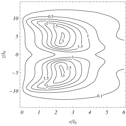
(a)

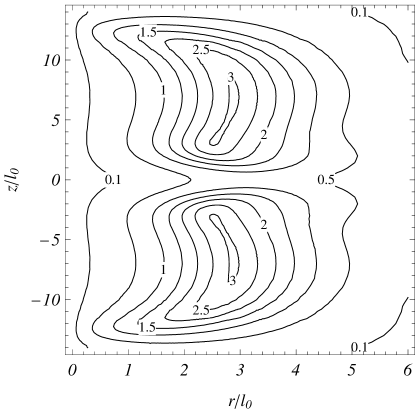
(b)

Figure 2: Contours of the angle $\theta$ of a soliton configuration for two values of the parameter $h$ with constant $\chi=1.96$: $h=0.60$ (a), $h=0.62$ (b).

In calculations using the method described here it is necessary every time to specify the value of the integral (8) and the parameter $\chi$. And only if the calculation leads to a positive result (to a soliton solution) can be calculate a corresponding value of the parameter $h$. In addition, if minimizing the functional does not yield a soliton solution, this does not mean the latter is nonexistent. This sort of situation can arise, for example, when the modelling region is not the right size (the soliton is too big). In light of this, only points corresponding to positive results are plotted in Fig.1.

Figure 3: $\theta$ as a function of the coordinate $r$ at $z=0$ for a soliton with the parameters of a ferromagnetic medium $\chi=1.57$, $h=0.25$.

(a)

(b)

Figure 4: Soliton energy as a function of the parameter $h$ for two values of the parameter $\chi$ for a ferromagnetic medium: 1.571 (a) and 1.963 (b). The points indicate the results of numerical calculations.

Figure 2 shows contours of constant angle $\theta$ for a typical soliton in the $(r,z)$ half plane for two values of the external magnetic field. In a three-dimensional space a constant value of the angle $\Theta$ corresponds to one or several toroids with a complicated envelope.

The profile $\theta(r,z)$ of a soliton for $z=0$ shown in Fig.3 shows that the characteristic size of the localized structures being studied here is on the order of $10l_{0}$.

Figure 4 is a plot of the energy of the soliton as a function of the external magnetic field. As the magnetic field is increased, the energy also rises. As these graphs show, to excite a soliton with a given energy in a material with a higher value of $D$, it is necessary to increase the external magnetic field strength $H_{0}$.

It turned out that all the solitons that were found are stable with respect to scaling perturbations:

$$\dfrac{d^{2}}{d\lambda^{2}}E({\bf m}({\bf r}+\lambda\,{\bf r}))\Bigr{|}_{\lambda=0}>0,$$ (21)

$$\dfrac{d^{2}}{d\lambda^{2}}E({\bf m}(x+\lambda\,x,y,z))\Bigr{|}_{\lambda=0}>0,$$ (22)

$$\dfrac{d^{2}}{d\lambda^{2}}E({\bf m}(r,\varphi,z+\lambda\,z))\Bigr{|}_{\lambda=0}>0,$$ (23)

$$\dfrac{d^{2}}{d\lambda^{2}}E({\bf m}(r+\lambda\,r,\varphi,z))\Bigr{|}_{\lambda=0}>0.$$ (24)

Nevertheless, the extrema that were found do not provide a minimum for the energy functional (5) in a strict mathematical sense. We examined the stability of the solitons with respect to small perturbations. A special type of functions $\delta\phi(r,z)$ and $\delta\theta(r,z)$ (complex perturbations) was found such that

$$\dfrac{d^{2}}{d\lambda^{2}}E(\phi+\lambda\,\delta\phi,\theta+\lambda\,\delta\theta)\Bigr{|}_{\lambda=0}<0.$$ (25)

However, even if the structures being studied here turn out to be unstable, they may have a rather long lifetime.

III III. ASYMPTOTIC BEHAVIOR

Data from the numerical calculations show that with distance from the center of a soliton the azimuthal angle of the vector ${\bf n}$ (14) becomes a linear function of the coordinate $z$, i.e. $\phi(r,z)\rightarrow 2\pi m+\pi/2+kz$ as $|{\bf r}|\rightarrow\infty$, $m\in{\mathbb{Z}}$. In addition, the soliton structure found as a result of minimization shows that $\theta(0,z)=0$. Since the angle $\theta$ goes monotonically to zero as $|{\bf r}|\rightarrow\infty$, the initial system of Eqs. (17) and (18) can be linearized for small $\theta$ with larger values of $|{\bf r}|$:

$$-\left(k^{2}-\frac{4\chi k}{\pi l_{0}}+\frac{1+h}{{l_{0}}^{2}}+\frac{1}{r^{2}}\right)\theta+\Delta_{2}\theta=0$$ (26)

$$(-(4\chi/\pi l_{0})+2k){\partial_{z}}{\theta}=0.$$ (27)

It follows at once from (27) that the constant k is determined by the Dzyaloshinsky constant, as

$$k=2\chi/(\pi l_{0})=D/\alpha.$$ (28)

Using the auxiliary function

$$\psi(r,z,\varphi)=\theta(r,z)cos(\varphi)$$ (29)

it is convenient to rewrite Eq. (26) in the form

$$\Delta\psi=\gamma^{2}\psi,$$ (30)

where $\Delta$ is the laplacian operator in three dimensional space and

$$\gamma=\sqrt{1+h-(4\chi^{2}/\pi^{2})}/{l_{0}}.$$ (31)

We shall seek a solution for (29) and (30) subject to the conditions

$$\begin{cases}\theta\geqslant 0,r\geqslant 0,\\ \theta(0,z)=0,\\ \theta\rightarrow 0\quad(|{\bf r}|\rightarrow\infty),\\ \theta(r,-z)=\theta(r,z).\end{cases}$$ (32)

Note that in the special case of $\gamma=0$, Eq.(30) transforms to the Laplace equation

$$\Delta\psi=0,$$ (33)

and has an interesting electrostatic analog: the function $\psi$ is the potential for the electric field of a system consisting of charges distributed along a circle of arbitrary, but finite, radius $r=a$, at $z=0$, with a linear density proportional to $cos(\varphi)$ and an infinitely long, grounded filament passing along the axis of symmetry, where the potential of the filament, like the potential at infinity, is zero. In fact, Eq.(33) permits separation of variables in toroidal coordinates $(u,v,\varphi)$,

$$tanh(u) =(2ar)/(a^{2}+r^{2}+z^{2}),\quad 0\leqslant u<\infty,$$ (34)

$$cot(v) =(a^{2}-r^{2}-z^{2})/(2az),\quad 0\leqslant v<2\pi,$$ (35)

and has the exact solution bib:Andrews :

$$\psi=C\sqrt{a/r}Q_{1/2}(\chi)cos(\varphi),\\$$ (36)

where $C$ is an arbitrary positive constant, $\chi=coth(u)$, $Q_{1/2}(\chi)$ is the Legendre function of the second kind of order $1/2$. This function can be written as the integral bib:Lebedev :

$$Q_{1/2}(\chi)=\int_{0}^{\pi}{\frac{cos\xi}{\sqrt{2\chi-2cos\xi}}}{d\xi}={}\\ {}=\chi k_{\chi}K(k_{\chi})-\frac{2}{k_{\chi}}E(k_{\chi}),\quad k_{\chi}=\sqrt{\frac{2}{1+\chi}},$$ (37)

where $K$ and $E$ are the complete elliptical integrals of the first and second kind, respectively. The solution (36), like every linear combination of similar solutions, satisfies Eq. (32) and yields the following asymptotic representation for the function

$$\theta(r,z)\sim(r^{2}+z^{2})^{-3/2}r\quad(|{\bf r}|\rightarrow\infty),\quad\gamma=0.$$ (38)

The result (38) can be derived formally in another way. If $\vartheta$ is the polar angle of the spherical coordinate system $(\rho,\vartheta,\varphi)$ with $\rho=|{\bf r}|=\sqrt{r^{2}+z^{2}}$, then separating the variables in (33) and using (29) yields a basis of the functions of the form

$$\psi_{n}=C\rho^{-n-1}P_{n}^{1}(cos\vartheta)cos(\varphi).$$ (39)

Given the imposed conditions (32), $n$ is a positive odd number and in the asymptotic limit, only $n=1$ “survives”. This immediately yields the asymptote (38).

If $\gamma\neq 0$, then the Helmholtz equation (30) is solved by separation of variables in spherical coordinates. Then, given (29), we find the basis of the functions in the form

$$\psi_{n}=\frac{C}{\sqrt{\rho}}K_{n+1/2}(\gamma\rho)P_{n}^{1}(cos\vartheta)cos(\varphi),$$ (40)

where $K_{\nu}(\chi)$ is the modified Bessel function of the second kind. As a result, we obtain the final formula for the asymptotic behavior:

$$\theta(r,z)\sim\frac{(1+\gamma\sqrt{r^{2}+z^{2}})\,r}{e^{\gamma\sqrt{r^{2}+z^{2}}}(r^{2}+z^{2})^{3/2}}\quad(|{\bf r}|\rightarrow\infty).$$ (41)

This implies the necessary condition for the existence of a three-dimensional vortex soliton: $\gamma>0$. Then, according to (31),

$$1+h-(4\chi^{2}/\pi^{2})>0.$$ (42)

This result is in qualitative agreement with the plot in Fig.1. Note that this condition is the instability criterion for a helicoidal structure in uniaxial magnets bib:BarStef .

When the condition

$$1+h-(4\chi^{2}/\pi^{2})<0,$$ (43)

holds, the ground state of the hamiltonian (5) corresponds to the helicoidal structure

$$cos(\Theta)=\frac{h}{(4\chi^{2}/\pi^{2})-1},\quad\Phi=kz,$$ (44)

where the step size of the spiral $\lambda=2\pi/k$ and $k$ is the same as in (28). This sort of structure can be classified as a ferromagnetic spiral (FS) bib:Izumov1 ; bib:Izumov2 . Here the energy density

$$w=-\frac{{M_{0}}^{2}\beta}{2\pi^{2}}\frac{(1+h-(4\chi^{2}/\pi^{2}))^{2}}{(4\chi^{2}/\pi^{2})-1}.$$ (45)

This implies that the condition (42) holds, a uniform stable state $\theta=0$ is realized in the system. Thus, the solitons we have been studying are localized excitations of a uniform state.

The volume energy density of the soliton, $w$, falls off exponentially with distance from the center of the soliton, i.e.,

$$w(\rho,\vartheta)\sim-\frac{cos(k\rho\,cos\vartheta)(sin\vartheta)^{2}}{e^{\gamma\rho}\rho}\quad(\rho\rightarrow\infty).$$ (46)

IV IV. THE TOPOLOGY OF VORTEX SOLITONS

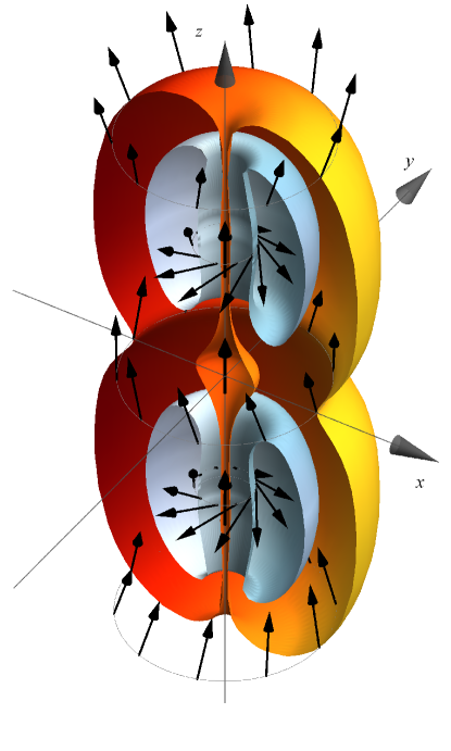
Figure 5: The distribution of the magnetization for a soliton with $h=0.11$, $\chi=1.37$. The toroids constructed in the interval $0<\varphi<\pi$ correspond to two values of the angle $\Theta$: for the outer toroid $\Theta=0.3$ and for the inner, $\Theta=2.0$

The unit vector field ${\bf m}$ is continuous and specified at each point of ${\mathbb{R}}^{3}$ space, while in the asymptotic limit ${\bf m}\rightarrow(0,0,1)$ as $|{\bf r}|\to\infty$. These kinds of fields map the space ${\mathbb{R}}^{3}\cup\{\infty\}$ onto a two-dimensional sphere ${\mathbb{S}}^{2}$ are classified as belonging to homotopic class $\pi_{3}({\mathbb{S}}^{2})={\mathbb{Z}}$, and are characterized by an integral Hopf index $H$:

$$H=-\frac{1}{(8\pi)^{2}}\int{\bf F}\cdot{\bf A}\,d{\bf r},$$ (47)

where $F_{i}=\epsilon_{ijk}{\bf m}\cdot(\nabla_{j}{\bf m}\times\nabla_{k}{\bf m})$ and $(\nabla\times{\bf A})=2{\bf F}$. The expression for the Hopf index $H$ of the fields (11) simplifies bib:KUR ; bib:Glad to

$$H=\frac{1}{4\pi}\int_{-\infty}^{\infty}{\int_{0}^{\infty}{{\bf n}\cdot\left[{\partial}_{r}{\bf n}\times{\partial}_{z}{\bf n}\right]}d{r}}d{z}.$$ (48)

If the index $H$ in (48) is nonzero, then the soliton can be classified as a toroidal hopfion bib:Kamchatnov ; bib:KBK ; bib:Fadd2 ; bib:KUR ; bib:Glad ; bib:BorRyb2 . A numerical calculation shows that for all the solitons obtained here, $H=0$. An example of a nontopological soliton with $H=0$ is a vortexfree magnon droplet bib:IvKos1 . For the class of objects studied here, as in Fig.5, one can see a structure of vortex wheels. The solitons found here can be classified as topological in the sense that they form an ensemble of “hopfion-antihopfion” pairs.

V V. CONCLUSION

It has been shown here that, within a definite region of parameters, three-dimensional vortex solitons can exist in incommensurate magnetically ordered crystals. The structure of topological solitons with a nonzero Hopf index $H$ (hopfions) will be described in later papers. The static solitons obtained here do not have the disadvantages of precessing magnon droplets bib:IvKos2 . Thus, despite their possible instability, they may have a sufficiently long lifetime that they can be observed in real experiments. In particular, if the external magnetic field is changed suddenly to a state (42) for a stable helicoidal structure (44), then the magnet will end up in an unstable phase and the transition to a uniform state may be accompanied by the appearance of solitons. It is also possible that within some range of the parameters $\chi-h$ that has not been studied in this paper, solitons of this type will be stable from a mathematical standpoint.

We thank B. A. Ivanov for the invitation to submit this article for the issue of this journal devoted to the 80-th birthday of V. G. Bar yakhtar, whose scientific activity and school have always made significant contributions to the development of the physics of magnetic phenomena.

References

- (1) Yu. A. Izyumov, Usp. Fiz. Nauk 144, 439 (1984) [ Sov. Phys. Usp. 27, 845 (1984)].
- (2) Yu. A. Izyumov, Neutron Diffraction on Long-period Structures [in Russian], Energoatomizdat, Moscow (1987).
- (3) I. E. Dzyaloshinsky, Zh. Eksp. Teor. Fiz. 46, 1420 (1964) [JETP 19, 960 (1964)].
- (4) I. E. Dzyaloshinsky, Zh. Eksp. Teor. Fiz. 47, 992 (1964) [JETP 20, 665 (1964)].
- (5) V. G. Bar’yakhtar, E. P. Stefanovsky, Fiz. Tverd. Tela 11, 1946 (1969) [Sov. Phys. Solid State 11, 1566 (1970)]
- (6) A. B. Borisov, V. V. Kiselev, Physica D. 31, 49 (1988).
- (7) A. B. Borisov, V. V. Kiselev, Physica D. 111, 96 (1998).
- (8) A. N. Bogdanov, D. A. Yablonsky, Zh. Eksp. Teor. Fiz. 95, 178 (1989) [JETP 68, 101 (1989)].
- (9) A. N. Bogdanov, M. V. Kudinov, D. A. Yablonsky, Fiz. Tverd. Tela 31, 99 (1989) [Sov. Phys. Solid State 31, 1707 (1989)].
- (10) A. Bogdanov, A. Hubert, JMMM 138, 255 (1994).
- (11) A. Bogdanov, A. Hubert, Phys. Stat. Sol. (b) 186, 527 (1994).
- (12) N. R. Cooper, Phys. Rev. Lett. 82, 1554 (1999).
- (13) T. Ioannidou, P. M. Sutcliffe, Physica D 150, 118 (2001).
- (14) A. B. Borisov, F. N. Rybakov, Pisma v Zh. Eksp. Teor. Fiz. 90, 593 (2009) [JETP Lett. 90, 544 (2009)].
- (15) B. A. Ivanov, A. M. Kosevich, Pisma v Zh. Eksp. Teor. Fiz. 24, 495 (1976) [JETP Lett. 24, 454 (1976)].
- (16) B. A. Ivanov, A. M. Kosevich, Zh. Eksp. Teor. Fiz. 72, 2000 (1977) [JETP 45, 1050 (1977)].
- (17) I. E. Dzyloshinskii, B. A. Ivanov, Pisma v Zh. Eksp. Teor. Fiz. 29, 592 (1979) [JETP Lett. 29, 540 (1979)].
- (18) A. B. Borisov, F. N. Rybakov, Pisma v Zh. Eksp. Teor. Fiz. 88, 303 (2008) [JETP Lett. 88, 264 (2008)].
- (19) R. H. Hobart, Proc. Phys. Soc. 82, 201 (1963).
- (20) G. M. Derrick, J. Math. Phys 5, 1252 (1964).
- (21) R. Rajaraman, Solitons And Instantons: An Introduction To Solitons And Instantons In Quantum Field Theory, North-Holland, (1982).
- (22) I. E. Dzyaloshinsky, Zh. Eksp. Teor. Fiz. 32, 1547 (1957) [JETP 5, 1259 (1957)].
- (23) I. Dzyaloshinsky, J. Phys. Chem. Solids 4, 241 (1958).
- (24) T. Moriya, Phys. Rev. 120, 91 (1960).
- (25) A. Bogdanov, Pisma v Zh. Eksp. Teor. Fiz. 62, 231 (1995) [JETP Lett. 62, 247 (1995)].
- (26) A. Bogdanov, Pisma v Zh. Eksp. Teor. Fiz. 68, 296 (1998) [JETP Lett. 68, 317 (1998)].
- (27) M. Andrews, J. of Electrostatics 64, 664 (2006).
- (28) N. N. Lebedev, Special Functions and their Applications, Prentice-Hall, London, (1965).
- (29) A. Kundu and Y. P. Rybakov, J. Phys. A 15, 269 (1982).
- (30) J. Gladikowski, M. Hellmund, Phys. Rev. D 56, 5194 (1997).
- (31) A. M. Kamchatnov, Zh. Eksp. Teor. Fiz. 82, 117 (1982) [JETP 55, 69 (1982)].
- (32) A. M. Kosevich, B. A. Ivanov and A. S. Kovalev, Phys. Rep. 194, 117 (1990).
- (33) L. D. Faddeev, A. J. Niemi, Nature 387, 58 (1997).