Cockcroft-11-16

Bending a Beam to Significantly Reduce Wakefields of Short Bunches

Abstract

A method of significantly reducing wakefields generated at collimators is proposed, in which the path of a beam is slightly bent before collimation. This is applicable for short bunches and can reduce the wakefields by a factor of around 7 for present day free electron lasers and future colliders.

Electromagnetic wakefields are created when an accelerated bunch of charged particles passes a discontinuity in the metallic structure of the beam pipe. Fields caused by geometric discontinuities, for example in cavities and collimators, are known as geometric wakefields, and can induce instabilities and emittance growth in the particle beam. As a result there is much interest in methods for reducing the geometric wakefields produced by a charged bunch of particles passing through a collimator. The customary approach is to reduce the taper angle of the collimator. Early work on the calculation of wakefields from smoothly tapered structures was pioneered by Yokoya Yokoya90 , Warnock Warnock93 and Stupakov Stupakov96 ; Stupakov01 . More recent investigations by Stupakov, Bane and Zagorodnov Stupakov07 ; Bane07 ; Bane10 and Podobedov and Krinsky Podobedov06 ; Podobedov07 have also looked at the effect of altering the transverse cross section of the collimator. A detailed analysis of the numerical and analytic calculation of collimator wakefields, including an informative introduction to the topic, may be found in Smith11 .

In this article an alternative approach is suggested whereby geometric wakefields are reduced by altering the path of the beam prior to collimation. This approach is facilitated by the highly relativistic regime in which lepton accelerators operate, where as shown in the following, the Coulomb field given from the Liénard-Wiechert potential is highly collimated in the direction of motion. It turns out the standard pancake field associated with a highly relativistic particle takes a finite time to develop to a given width. Thus by placing the collimator sufficiently close to a bending dipole the radius of the pancake remains smaller than the width of the aperture of the collimator. Using this method reduction of wakefields by factors of around 7 are feasible for some present day energies and bunch lengths.

For a particle of charge $q$ undergoing arbitrary motion ${\boldsymbol{x}}(\tau)$, where $\tau$ is the particle’s proper time, the Liénard-Wiechert fields at point ${\boldsymbol{X}}$ and time $T$ are given Jackson99 by

$${\boldsymbol{E}}({\boldsymbol{X}},T)\!=\!{\boldsymbol{E}}_{\text{LW}}\Big{(}\!{\boldsymbol{X}}\!-\!{\boldsymbol{x}}(\tau_{R}),{\boldsymbol{\beta}}(\tau_{R}),{\boldsymbol{a}}(\tau_{R})\!\Big{)}$$ (1)

and

$${\boldsymbol{B}}({\boldsymbol{X}},T)\!=\!{\boldsymbol{B}}_{\text{LW}}\Big{(}\!{\boldsymbol{X}}\!-\!{\boldsymbol{x}}(\tau_{R}),{\boldsymbol{\beta}}(\tau_{R}),{\boldsymbol{a}}(\tau_{R})\!\Big{)}.$$ (2)

Here $\tau_{R}$ is the retarded proper time and ${\boldsymbol{x}}(\tau_{R})$ the position of the charged particle at the retarded proper time. The $3$-vectors

$${\boldsymbol{\beta}}(\tau)\!=\!\frac{1}{c\gamma}{\frac{d{\boldsymbol{x}}}{d\tau}},{\qquad\text{and}\qquad}{\boldsymbol{a}}(\tau)\!=\!\frac{1}{\gamma}{\frac{d{\boldsymbol{\beta}}}{d\tau}}$$

are the Newtonian velocity and acceleration divided by $c$, where $\gamma\!=\!\sqrt{1+\left\|{d{\boldsymbol{x}}/d\tau}\right\|^{2}/c^{2}}$. The functions ${\boldsymbol{E}}_{\text{LW}}$ and ${\boldsymbol{B}}_{\text{LW}}$ are given by

$${\boldsymbol{E}}_{\text{LW}}(\!{\boldsymbol{r}}\!,\!{\boldsymbol{\beta}}\!,\!{\boldsymbol{a}}\!)\!\!=\!\!\frac{q}{4\pi\epsilon_{0}}\!\Bigg{(}\!\frac{({{\boldsymbol{n}}}\!-\!{\boldsymbol{\beta}})}{\gamma^{2}\!\left\|{\boldsymbol{r}}\right\|^{2}\!(1\!-\!{\boldsymbol{\beta}}\cdot{{\boldsymbol{n}}})^{3}}\!+\!\frac{{{\boldsymbol{n}}}\times\Big{(}\!({{\boldsymbol{n}}}\!-\!{\boldsymbol{\beta}})\times{\boldsymbol{a}}\!\Big{)}}{c\!\left\|{\boldsymbol{r}}\right\|\!(1\!-\!{\boldsymbol{\beta}}\cdot{{\boldsymbol{n}}})^{3}}\!\Bigg{)}$$ (3)

and

$${\boldsymbol{B}}_{\text{LW}}({\boldsymbol{r}},{\boldsymbol{\beta}},{\boldsymbol{a}})=\frac{1}{c}{{\boldsymbol{n}}}\times{\boldsymbol{E}}_{\text{LW}}({\boldsymbol{r}},{\boldsymbol{\beta}},{\boldsymbol{a}}),$$ (4)

where ${\boldsymbol{r}}={\boldsymbol{X}}-{\boldsymbol{x}}(\tau_{R})$, ${{\boldsymbol{n}}}={\boldsymbol{r}}/\left\|{\boldsymbol{r}}\right\|$ and $\gamma=(1-\left\|{\boldsymbol{\beta}}\right\|^{2})^{-1/2}$. The first term in (3) will be referred to as the Coulomb field and the second term as the Radiative field.

For particles moving close to the speed of light, i.e. with high $\gamma$-factors and $\left\|{\boldsymbol{\beta}}\right\|\approx 1$, the denominator in (3) is very small when ${{\boldsymbol{n}}}$ is in the direction of ${\boldsymbol{\beta}}$. Hence ${\boldsymbol{E}}_{\text{LW}}({\boldsymbol{r}},{\boldsymbol{\beta}},{\boldsymbol{a}})$ is very large in the direction ${{\boldsymbol{n}}}\approx{\boldsymbol{\beta}}$ . FIG. 1 is a plot of the magnitude of the Coulomb and Radiative fields for fixed $\left\|{\boldsymbol{r}}\right\|$, ${\boldsymbol{\beta}}$ and ${\boldsymbol{a}}$ as a function of the spherical coordinates.

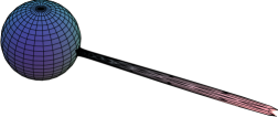
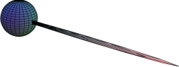
Coulomb field	Radiative field

Figure 1: The magnitude of the Coulomb and radiative fields for a high $\gamma$, given as height above the sphere. The bulk of the fields is in the direction of motion.

A relativistic particle undergoing nonlinear acceleration will generate a field primarily in the instantaneous direction of motion of the the particle. This is true not just for the radiation field, where it is usually described as a search light, but also for the Coulomb field. For high $\gamma$-factors the bulk of the fields, for both the Coulomb and radiation terms, is inside an angle $\Delta\phi\sim 1/\gamma$ where $\Delta\phi$ is the angle from the direction of motion. By contrast, the field generated by a relativistic particle moving with constant velocity is flattened towards the plane orthogonal to the direction of motion, and is often called a pancake field. It is reasonable to ask how these two radically different behaviours can be consistent.

Figure 2: Showing the communication between a particle and its pancake

Consider a particle moving at velocity $v$ along the horizontal line $PQ$ in FIG. 2. Let $R$ be a point in the pancake a distance $h$ from the particle, when the particle is at $Q$. The last point at which the particle could communicate with the point $R$ is at $P$, a length $v{t_{\text{s}}}$ from $Q$. Here ${t_{\text{s}}}$ is the time it takes for light to travel from $P$ to $R$ and also the time for the particle to travel from $P$ to $Q$. Then $\left\|PR\right\|=c{t_{\text{s}}}$ and $\left\|PQ\right\|=v{t_{\text{s}}}$. Thus $(c{t_{\text{s}}})^{2}=h^{2}+(v{t_{\text{s}}})^{2}$. Hence $h^{2}=c^{2}{t_{\text{s}}}^{2}(1-v^{2}/c^{2})=c^{2}{t_{\text{s}}}^{2}/\gamma^{2}$ so ${t_{\text{s}}}=\gamma h/c$ and $\left\|PQ\right\|=\gamma hv/c$. Thus a particle needs to have travelled in a straight line for a length $\left\|PQ\right\|=\gamma hv/c$ in order for a pancake of radius $h$ to develop. Looking at the fields which originate at $P$ and arrive at $R$, they are at an angle approximately $\left\|RQ\right\|/\left\|PR\right\|=1/\gamma$. This is consistent with FIG. 1.

This gives rise to a way to significantly reduce the wakefields generated when a bunch passes a cavity or collimator. The idea is to bend the beam slightly before it enters the structure. Most of the Coulomb field generated by the particle before the bend will continue in a straight line (see FIG. 3). By sufficiently enlarging the beam pipe in this direction the wakefield due to this part of the field can be neglected. If the distance, $Z$, of the straight line segment from the terminus of the bend to the centre of the collimator is sufficiently small, then the resulting pancake field will be too small to reach the sides of the structure. Of course bending the beam will generate additional radiation fields, however by judicious choice of geometry of the beam these can be minimized.

Figure 3: Suggested path of beam though collimator

Let $h$ denote half the aperture of the collimator and let $L$ represent the spatial length of the bunch. The following two scenarios will be considered:

• Long smooth bunches where $L>h$ and any variation in the density of the bunch is over length scales longer than $h$,

• Bunches where variation in density is over short length scales less than about $0.2h$. This includes the case of very short bunches where $L\ll 0.2h$.

These two scenarios are both applicable to present day machines, where the bunch length depends upon the specific objectives and engineering considerations of individual projects. In the following calculation it will be shown that for short bunches, or bunches with large amounts of micro-bunching, it is possible to make a significant reduction in wakefields. This is applicable to present day free electron lasers, which employ bunch compressors to produce very short bunches, for example in LCLS $L/c\approx 0.008$ps. Assuming a collimator of half aperture $h=0.5$mm then in this case $L=0.0048h$. It turns out that electromagnetic fields due to long smooth bunches may not be reduced significantly. In many present day colliders the bunches are designed to be long and smooth, however in the future short bunch colliders may be desirable (see TABLE 1).

Table 1: Bunch lengths for some modern colliders and FELs

Collider	Year of	Bunch length [ps]
	Commissioning
SLC, SLAC	$1989$	$3$
ILC	$\geq 2015$	$1$
CLIC	$\geq 2025$	$0.15$
Free Electron Laser		Min. bunch length [ps]
FLASH, DESY	$2005$	$0.05$
LCLS, SLAC	$2009$	$0.008$
XFEL, DESY	$2014$	$0.08$

Consider a bunch modelled as a one dimensional continuum of point particles where each particle undergoes the same motion in space but at a different time. This bunch is moving at a constant speed with relativistic factor $\gamma$. Let $\nu$ label the points in the bunch, which will be called body points. The profile of the bunch is given by $\rho(\nu)$. Let ${\boldsymbol{x}}(\tau)$ represent the path of the bunch where $\tau$ is the proper time. For each body point $\nu$,

$${\boldsymbol{x}}_{\nu}(\tau)={\boldsymbol{x}}(\tau),{\quad\text{and}\quad}t_{\nu}(\tau)=(\tau+\nu)/\gamma.$$ (5)

In the following all fields are measured at a fixed point ${\boldsymbol{X}}=(X,Y,Z)$. In FIG. 3, $X=0$ and $Y=h$. Let $\hat{\tau}({\boldsymbol{X}},T,\nu)$ represent the retarded time for the body point $\nu$ corresponding to the fields measured at ${\boldsymbol{X}}$ at laboratory time $T$. The retarded time condition is given by

$$cT-ct_{\nu}\big{(}\hat{\tau}({\boldsymbol{X}},T,\nu)\big{)}=\left\|{\boldsymbol{X}}-{\boldsymbol{x}}_{\nu}\big{(}\hat{\tau}({\boldsymbol{X}},T,\nu)\big{)}\right\|,$$ (6)

and hence

$$\!\!\!\!cT-c\hat{\tau}({\boldsymbol{X}},T,\nu)/\gamma-c\nu/\gamma=\left\|{\boldsymbol{X}}-{\boldsymbol{x}}\big{(}\hat{\tau}({\boldsymbol{X}},T,\nu)\big{)}\right\|.$$ (7)

Let $\hat{T}(\nu,\tau,{\boldsymbol{X}})$ represent the arrival time at ${\boldsymbol{X}}$ of the field generated by body point $\nu$ at proper time $\tau$. Thus

$$c\hat{T}(\nu,\tau,{\boldsymbol{X}}) =ct_{\nu}(\tau)+\left\|{\boldsymbol{X}}-{\boldsymbol{x}}_{\nu}(\tau)\right\|$$

$$=c(\tau+\nu)/\gamma+\left\|{\boldsymbol{X}}-{\boldsymbol{x}}(\tau)\right\|.$$ (8)

From (7) and (8)

$$cT =c\big{(}\hat{\tau}({\boldsymbol{X}},T,\nu)+\nu\big{)}/\gamma+\left\|{\boldsymbol{X}}-{\boldsymbol{x}}\big{(}\hat{\tau}({\boldsymbol{X}},T,\nu)\big{)}\right\|$$

$$=c\hat{T}(\nu,\hat{\tau}({\boldsymbol{X}},T,\nu),{\boldsymbol{X}}).$$ (9)

Since $\hat{T}$ is increasing and the range of $\hat{\tau}$ is from $-\infty$ to $+\infty$ it follows that $\hat{T}$ and $\hat{\tau}$ are inverse to each other, yielding (9) and

$$\hat{\tau}({\boldsymbol{X}},\hat{T}(\nu,\tau,{\boldsymbol{X}}),\nu)=\tau.$$ (10)

Let us set

$$\hat{\tau}_{0}({\boldsymbol{X}},T)\!=\!\hat{\tau}({\boldsymbol{X}},T,0){\quad\text{and}\quad}\hat{T}_{0}(\tau,{\boldsymbol{X}})\!=\!\hat{T}(0,\tau,{\boldsymbol{X}}).$$ (11)

Then $\hat{T}(\nu,\tau,{\boldsymbol{X}})$ and $\hat{\tau}({\boldsymbol{X}},T,\nu)$ may be written in terms of $\hat{T}_{0}(\tau,{\boldsymbol{X}})$ and $\hat{\tau}_{0}({\boldsymbol{X}},T)$. From (8)

$$\hat{T}(\nu,\tau,{\boldsymbol{X}})\!=\!\hat{T}_{0}(\tau,{\boldsymbol{X}})\!+\!\nu/\gamma.$$ (12)

From (9), (10) and (11),

$$\hat{T}_{0}(\hat{\tau}_{0}({\boldsymbol{X}},T),{\boldsymbol{X}})=T$$ (13)

and

$$\hat{\tau}_{0}({\boldsymbol{X}},\hat{T}_{0}(\tau,{\boldsymbol{X}}))=\tau.$$ (14)

Substituting (12) into (14) leads to

$$\hat{\tau}_{0}({\boldsymbol{X}},\hat{T}(\nu,\tau,{\boldsymbol{X}})-\nu/\gamma)=\tau.$$ (15)

Substituting $\tau=\hat{\tau}({\boldsymbol{X}},T,\nu)$ and using (9) yields

$$\hat{\tau}({\boldsymbol{X}},T,\nu)\!=\!\hat{\tau}_{0}({\boldsymbol{X}},T\!-\!\nu/\gamma).$$ (16)

For the body point $\nu$ the Liénard-Wiechert electric and magnetic fields at point ${\boldsymbol{X}}$ and time $T$ are given by substituting $\tau_{R}=\hat{\tau}({\boldsymbol{X}},T,\nu)$ into (1),

$${\boldsymbol{E}}(\!{\boldsymbol{X}}\!,\!T\!,\!\nu\!)\!=\!{\boldsymbol{E}}_{\text{LW}}\Big{(}\!\!{\boldsymbol{X}}\!-\!{\boldsymbol{x}}\big{(}\!\hat{\tau}(\!{\boldsymbol{X}}\!,\!T\!,\!\nu\!)\!\big{)},{\boldsymbol{\beta}}\big{(}\!\hat{\tau}(\!{\boldsymbol{X}}\!,\!T\!,\!\nu\!)\!\big{)},\!{\boldsymbol{a}}\big{(}\!\hat{\tau}(\!{\boldsymbol{X}}\!,\!T\!,\!\nu\!)\!\big{)}\!\Big{)}$$

and likewise for ${\boldsymbol{B}}({\boldsymbol{X}},T,\nu)$. Let ${\boldsymbol{E_{0}}}({\boldsymbol{X}},T)$ be the electric field at point ${\boldsymbol{X}}$ and time $T$ due to the body point $\nu=0$ given by

$${\boldsymbol{E_{0}}}({\boldsymbol{X}},T)={\boldsymbol{E}}_{\text{LW}}\Big{(}\!{\boldsymbol{X}}\!-\!{\boldsymbol{x}}\big{(}\!\hat{\tau}_{0}(\!{\boldsymbol{X}}\!,\!T\!)\!\big{)}\!,\!{\boldsymbol{\beta}}\big{(}\!\hat{\tau}_{0}(\!{\boldsymbol{X}}\!,\!T\!)\!\big{)}\!,\!{\boldsymbol{a}}\big{(}\!\hat{\tau}_{0}\!(\!{\boldsymbol{X}}\!,\!T\!)\!\big{)}\!\Big{)}$$

Using (16) it follows

$${\boldsymbol{E}}({\boldsymbol{X}},T,\nu) \!={\boldsymbol{E_{0}}}({\boldsymbol{X}},T-\nu/\gamma).$$

The total electric field at the point ${\boldsymbol{X}}$ at time $T$ is given by

$${\boldsymbol{E}}_{\textup{Tot}}({\boldsymbol{X}},T) =\int\rho(\nu){\boldsymbol{E}}({\boldsymbol{X}},T,\nu)d\nu$$

$$=\int\rho(\nu){\boldsymbol{E_{0}}}({\boldsymbol{X}},T-\nu/\gamma)d\nu$$

$$=\int\gamma\rho\big{(}\gamma(T-T^{\prime})\big{)}{\boldsymbol{E_{0}}}({\boldsymbol{X}},T^{\prime})dT^{\prime}$$

$$=\int{\rho_{\textup{Lab}}}(T-T^{\prime}){\boldsymbol{E_{0}}}({\boldsymbol{X}},T^{\prime})dT^{\prime},$$

where $T^{\prime}=T-\nu/\gamma$, and $q{\rho_{\textup{Lab}}}(T)=q\gamma\rho(\gamma T)$ is the charge density as measured in the laboratory frame. Thus the key result is that the total electric field is given by the convolution

$${\boldsymbol{E}}_{\textup{Tot}}({\boldsymbol{X}},T) =\int{\rho_{\textup{Lab}}}(T-T^{\prime}){\boldsymbol{E_{0}}}({\boldsymbol{X}},T^{\prime})dT^{\prime}.$$ (17)

The above can be repeated for the total magnetic field ${\boldsymbol{B}}_{\text{Tot}}({\boldsymbol{X}},T)$. Clearly ${\boldsymbol{E_{0}}}({\boldsymbol{X}},T^{\prime})$ will depend on the energy of the beam $\gamma$ and the path of the beam ${\boldsymbol{x}}(\tau)$. The energy of the beam is fixed, therefore the only permitted freedom is to alter the position of the collimator and hence change ${\boldsymbol{X}}$, or to modify the path of the beam.

Consider the path constructed from a straight line followed by an arc of a circle of radius $R$ followed by another straight line. Let $\Theta$ denote the angle of arc. The coordinate system is chosen so that the direction of the second straight line is along the $z$ axis and the arc is in the $x-z$ plane, finishing at the origin. The trajectory ${\boldsymbol{x}}_{\nu}(\tau)={\boldsymbol{x}}(\tau)=\big{(}x(\tau),y(\tau),z(\tau)\big{)}$ is given in TABLE 2. The point ${\boldsymbol{X}}$ is given as ${\boldsymbol{X}}=\big{(}X,Y,Z\big{)}$ with $Z>0$. Thus the field measured is a function of ${\boldsymbol{X}}$, $\Theta$, $R$ and the time the field arrives, $T$.

Table 2: The trajectory for a particle in the bunch

trajectory		domain
	$R(\cos\Theta\!-\!1)\!+\!(\Theta R\!+\!\gamma v\tau)\sin\Theta$	$-\infty<\tau<-{R\Theta}/{\gamma v}$
$x(\tau)$	$R\Big{(}\!\cos({\gamma v\tau}/{R})\!-\!1\!\Big{)}$	$-{R\Theta}/{\gamma v}<\tau<0$
	$0$	$0<\tau<\infty$
$y(\tau)$	$0$	$-\infty<\tau<\infty$
	$-R\sin\Theta\!+\!(\Theta R\!+\!\gamma v\tau)\cos\Theta$	$-\infty<\tau<-{R\Theta}/{\gamma v}$
$z(\tau)$	$R\sin({\gamma v\tau}/{R})$	$-{R\Theta}/{\gamma v}<\tau<0$
	$\gamma v\tau$	$0<\tau<\infty$

Straight path	Pre-bent path.

Figure 4: The electric field strength $||{\boldsymbol{E_{0}}}({\boldsymbol{X}},T)||$ at ${\boldsymbol{X}}=(0,h,10h)$, with $h=0.5$mm, due to a body point following a straight path along the $z$-axis and a body point following the pre-bent path given in TABLE 2 with $\Theta=0.13$rad and $R=0.5$m.

Consider the two cases given in FIG. 4 in which $\gamma=1000$, $X=0$, $Y=h$ and $Z=10h$. In the straight line case the peak field is $\approx 75$Vm^-1 and the majority of the field arrives within an interval of $0.015$ps. In fact it is easy to show that for a straight line path the peak field increases with $\gamma$ and the width decreases with $\gamma$ leading to the classic pancake. By contrast for the pre-bent case the peak field is significantly reduced to only $\approx 7.7$Vm^-1, however the interval over which the field arrives is now $0.35$ps for the right hand peak, and $0.1$ps for the left hand peak. The reason for these two peaks is that the left hand peak is the coulomb field due to the first straight line segment, whereas the second peak is due to the radiation from the circular part of the beam path. The discontinuity is a result of the discontinuity in acceleration for this trajectory. Repeating the calculation with higher $\gamma$-factors doesn’t significantly change the height or shape of the second peak.

If the bunch is long and smooth, i.e. longer than the collimator aperture, so that there is no significant change in ${\rho_{\textup{Lab}}}$ over the width of ${\boldsymbol{E_{0}}}({\boldsymbol{X}},T^{\prime})$, then ${\boldsymbol{E_{0}}}({\boldsymbol{X}},T^{\prime})$ may be crudely regarded as a $\delta$-function and ${\boldsymbol{E}}_{\textup{Tot}}({\boldsymbol{X}},T)$ is given by

$${\boldsymbol{E}}_{\textup{Tot}}({\boldsymbol{X}},T) \approx{\rho_{\textup{Lab}}}(T)\int{\boldsymbol{E_{0}}}({\boldsymbol{X}},T^{\prime})dT^{\prime}.$$ (18)

Integration of ${\boldsymbol{E_{0}}}({\boldsymbol{X}},T^{\prime})$ for the straight and pre-bent trajectories reveals that

$$||{\boldsymbol{E}}_{\textup{Tot}}({\boldsymbol{X}},T)||\approx\frac{q}{2\pi\epsilon_{0}c}\frac{{\rho_{\textup{Lab}}}(T)}{||{\boldsymbol{X}}||}$$ (19)

This value of ${\boldsymbol{E}}_{\textup{Tot}}$ is independent of $R$ and $\Theta$ for all paths where $R$ is large compared to $L$. To see why this is the case consider our one dimensional beam of particles as a continuous flow of charge, similar to a line charge in a wire but without the background ions. The fields due to this flow may be calculated using the Biot-Savart law. Since $h\ll R$ the field is dominated by the nearby current and hence no variation of $R$, $\Theta$ or $Z$ will alter the fields.

Table 3: Peak field strength for different sized bunches with h=0.5mm.

Bunch Length		Peak $||{\boldsymbol{E}}_{\textup{Tot}}({\boldsymbol{X}},T)||$ [Vm-1]
L[h]	(L/c)[ps]	straight	pre-bent
$1.8\times 10^{1}$	$3.00\times 10^{0}$	$1.97\times 10^{-1}$	$1.97\times 10^{-1}$
$6.00\times 10^{-1}$	$1.00\times 10^{0}$	$5.91\times 10^{-1}$	$5.89\times 10^{-1}$
$9.00\times 10^{-2}$	$1.50\times 10^{-1}$	$3.93\times 10^{0}$	$3.48\times 10^{0}$
$4.80\times 10^{-2}$	$8.00\times 10^{-2}$	$7.33\times 10^{0}$	$5.27\times 10^{0}$
$3.00\times 10^{-2}$	$5.00\times 10^{-2}$	$1.16\times 10^{1}$	$6.36\times 10^{0}$
$4.80\times 10^{-3}$	$8.00\times 10^{-3}$	$5.12\times 10^{1}$	$7.53\times 10^{0}$

If the beam has bunches of length $L\lesssim 0.05h$ then it follows from (17) and FIG. 4 that a considerable reduction in fields is possible. It is straightforward to calculate ${\boldsymbol{E}}_{\textup{Tot}}({\boldsymbol{X}},T)$ numerically using a Gaussian particle distribution $\rho_{\text{Lab}}$ for the two cases in FIG. 4 (see TABLE 3). If $\rho_{\text{Lab}}$ has full width at half maximum $L/c=0.008ps$ with corresponding bunch length $L=0.0048h$, then the peak value for the total electric field in the straight line case is given by $\approx 51.2\textup{Vm}^{-1}$. By contrast, in the pre-bent case the peak value for the total electric field is $\approx 7.5\textup{Vm}^{-1}$, giving an approximate factor of 7 reduction in field. This is approaching the maximal factor of 10 improvement one can achieve with $\gamma=1000$, which occurs when the bunch length is small enough that the convolution gives the peak values for the fields in FIG. 4. With higher energies and shorter bunch lengths the radiation peak remains unchanged, whereas the electric field for the straight path grows linearly with $\gamma$. Thus even greater improvements can be made.

In the above calculation the specific field point ${\boldsymbol{X}}=(0,h,10h)$ is chosen and the peak electric fields are minimized for this particular point on the collimator. If instead the point is displaced in the positive $x$ direction (FIG 3), then a significant increase in field strength is observed. This increase results from both the Coulomb field from the straight section of the path before the arc and the radiation from the circular part of the path. It will be necessary to alter the shape of the collimator to avoid these high fields interacting with the material in the collimator. This need not affect the efficacy of the collimator to remove the halo, for example see FIG 5. The optimum design of the beam path, beam tube and collimator shape, for particular machines will require a combination of analytic, numerical and experimental research. Clearly long tapers will reduce the advantage gained by bending the beam since it will give time for the pancake to form. However it may be advantageous to use a short taper.

Figure 5: Modified collimator in the plane transverse to the path of the beam.

The placing of an additional bending dipole just before a collimator would inevitably cause unwanted losses in beam energy due to radiation loss. However all accelerators, even Linacs, already have to bend the beam using dipoles in certain places. Therefore it seems natural to place a collimator directly after a bending magnet in order not to lose any more beam energy through radiation loss.

The authors acknowledge support from the Cockcroft Institute (STFC ST/G008248/1) and the Alpha X project Strathclyde University. They are grateful to Dr D. A. Burton Lancaster University, and Dr A. Noble Strathclyde University for valuable discussions.

References

• [1] K. Yokoya. Impedence of slowly tapered structures. CERN Report, (SL-90-88-AP), 1990.
• [2] R. L. Warnock. An intergo-algebraic equation for high frequency wake fields in a tube with smoothly varying radius. SLAC Report, (SLAC-PUB-6038), 1993.
• [3] G. V. Stupakov. Geometrical wake of a smooth flat collimator. SLAC Report, (SLAC-PUB-7167), 1996.
• [4] G. V. Stupakov. Impedance of small-angle collimators in high-frequency limit. SLAC Report, (SLAC-PUB-8857), 2001.
• [5] G. Stupakov. Low frequency impedance of tapered transitions with arbitrary cross sections. Phys. Rev. ST Accel. Beams, 10(9):094401, Sep 2007.
• [6] K. L. F. Bane, G. Stupakov, and I. Zagorodnov. Impedance calculations of nonaxisymmetric transitions using the optical approximation. Phys. Rev. ST Accel. Beams, 10(7):074401, Jul 2007.
• [7] G. Stupakov, K. L. F. Bane, and I. Zagorodnov. Impedance scaling for small angle transitions. Phys. Rev. ST Accel. Beams, 14(1):014402, Jan 2011.
• [8] B. Podobedov and S. Krinsky. Transverse impedance of axially symmetric tapered structures. Phys. Rev. ST Accel. Beams, 9(5):054401, May 2006.
• [9] B. Podobedov and S. Krinsky. Transverse impedance of tapered transitions with elliptical cross section. Phys. Rev. ST Accel. Beams, 10(7):074402, Jul 2007.
• [10] J. D. A. Smith. Calculations of Collimator Wakefield. PhD thesis, Lancaster University, UK, 2011.
• [11] J D Jackson. Classical Electrodynamics (3rd Edition). Wiley, 1999.