Uncertainties and systematics in stellar evolution models of Red Giant Stars

Abstract

In this last decade, our knowledge of evolutionary and structural properties of stars of different mass and chemical composition has significantly improved. This notwithstanding, updated stellar models are still affected by significant and, usually, not negligible uncertainties. These uncertainties are related to our poor knowledge of some physical processes occurring in the real stars such as the efficiency of mixing processes. These drawbacks of stellar models have to be properly taken into account when comparing theory with observations. In this paper we briefly review current uncertainties affecting low-mass stellar models, i.e. those structures with mass in the range between $0.6M_{\odot}$ and $\sim 1.4M_{\odot}$, during the Red Giant Branch stage.

1 Introduction

During the second half of last century, stellar evolution theory has allowed us to understand the Color Magnitude Diagram (CMD) of both galactic globular clusters (GGCs) and open clusters, so that now we can explain the distribution of stars in the observed CMDs in terms of the nuclear evolution of stellar structures and, thus, in terms of cluster age and chemical composition. In recent years, however, the impressive improvements achieved for both photometric and spectroscopic observations as well as asteroseismological measurements, has allowed us to collect data of an un-precedent accuracy, which provide at the same time a stringent test and a challenge for the accuracy of the models.

On the theoretical side, significant improvements have been achieved in the determination of the Equation of State (EOS) of the stellar matter, opacities, nuclear cross sections, neutrino emission rates, that are, the physical inputs needed in order to solve the equations of stellar structure.

The capability of current stellar models to account for all the observed evolutionary phases is undoubtedly an exciting achievement which crowns with success the development of stellar evolutionary theories as pursued all along the second half of the last century. Following such a success, one is often tempted to use evolutionary results in an uncritical way, i.e., taking these results at their face values without accounting for theoretical uncertainties. However, these uncertainties do exist, as it is clearly shown by the not negligible differences still existing among evolutionary results provided by different research groups (see the discussion in Chaboyer, 1995; Cassisi et al., 1998, 1999; Castellani & degl’Innocenti, 1999; Cassisi, 2004).

We will discuss the main ’ingredients’ necessary for computing stellar models and show how the uncertainties on these inputs affect theoretical predictions of the evolutionary properties of Red Giant Branch (RGB) low-mass stars.

2 Stellar evolution: the ingredients

The stellar structure equations are well known since long time, and a clear description of the physical meaning of each one of them can be found in several books (as, for instance, Kippenhahn & Weigert, 1990).

The (accurate) numerical solution of these differential equations is no longer a problem and it can be easily and quickly achieved when using modern numerical solution schemes and current generation of powerful computers. This notwithstanding, in order to solve these equations, boundary conditions have to be provided: the boundary condition at the stellar centre are trivial (Salaris & Cassisi, 2005, see); however the same does not apply for those at the stellar surface, i.e., the values of temperature and pressure at the base of the atmosphere. These boundary conditions can be obtained either by adopting an empirical relation for the thermal stratification like that provided by Krishna Swamy (1966) or a theoretical approximation as the so-called Eddington approximation. A more rigorous procedure is to use results from model atmosphere computations (VandenBerg et al., 2008).

In order to compute a stellar structure, it is fundamental to have an accurate description of the physical behaviour of the matter in the thermal conditions characteristics of the stellar interiors and atmospheres. This means that we need to know several physical inputs as: opacity, EOS, nuclear cross-sections, neutrino energy losses. A rich literature exists describing the improvements which have been achieved in this last decade concerning our knowledge of these physical inputs (Catelan, 2009; Cassisi et al., 1998, 1999; Salaris et al., 2002, and references therein).

Some important assumptions have also to be made concerning the efficiency of those mechanisms, such as atomic diffusion and radiative levitation, which can modify the chemical stratification in the interiors and atmosphere. Until few years ago, all these non-canonical processes were usually ignored in stellar models computations. However, helioseismology has clearly shown how important is to include atomic diffusion in the computation of the so-called Standard Solar Model (SSM), in order to obtain a good agreement between the observed and the predicted frequencies of the non-radial p-modes (Christensen-Dalsgaard et al., 1993). In the meantime, quite recent spectroscopical measurements for low-mass, metal-poor stars in GGCs strongly point out the importance of including radiative levitation in stellar computations in order to put in better agreement empirical estimates with the predictions provided by diffusive models.

When dealing with stellar model computations, one has also to account for the occurrence of mixing. Due to the poor knowledge of how to manage the mixing processes in a stellar evolutionary code, the efficiency of convection is commonly treated by adopting some approximate theory. In this context, it has to be noticed that when treating a region where convection is stable, one has to face with two problems: i) What is the ‘right’ temperature gradient in such region?, ii) What is the ‘real’ extension of the convective region?

The first question is really important only when considering the outer convective regions such as the convective envelopes of cool stars. This occurrence is due to the evidence that, in the stellar interiors as a consequence of the high densities and, in turn, of the high efficiency of energy transport by convective motions, the ‘real’ temperature gradient has to be equal to the adiabatic one. This consideration does not apply when considering the outer, low-density, stellar regions, where the correct temperature gradient has to be larger than the adiabatic one: the so-called superadiabatic gradient. One of the main problem in computing star models is related to the correct estimate of this superadiabatic gradient.

Almost all evolutionary computations available in literature rely on the mixing length theory (MLT Böhm-Vitense, 1958). It contains a number of free parameters, whose numerical values affect the model $T_{\rm eff}$; one of them is $\alpha_{\rm MLT}$, the ratio of the mixing length to the pressure scale height, which provides the scale length of the convective motions. There exist different versions of the MLT, each one assuming different values for these parameters. However, as demonstrated by Pedersen et al. (1990) and Salaris & Cassisi (2008), the $T_{\rm eff}$ values obtained from the different formalisms can be made consistent, provided that a suitable value of $\alpha_{\rm MLT}$ is selected. Therefore, at least for the evaluation of $T_{\rm eff}$, the MLT is basically a one-parameter theory. The value of $\alpha_{\rm MLT}$ is usually calibrated by reproducing the solar $T_{\rm eff}$, and this solar-calibrated value is then used for computing models of stars very different from the Sun (e.g. metal poor giants). It is worth recalling that there exists also an alternative formalism for the computation of the superadiabatic gradient: the so-called Full-Spectrum-Turbulence theory (FST Canuto et al., 1996), a MLT-like formalism with a more sophisticated expression for the convective flux, and the scale-length of the convective motion fixed a priori.

For low-mass stars, the problem of the real extension of a convective region really affects only the convective envelope. In the canonical framework it is assumed that the border of a convective region is fixed by the condition - according to the classical Schwarzschild criterion - that the radiative gradient is equal to the adiabatic one. However, it is clear that this condition fixes the point where the acceleration of the convective cells is equal to zero, so it is realistic to predict that the convective elements can move beyond, entering and, in turn, mixing the region surrounding the classical convective boundary. This process is commonly referred to as convective overshoot. Convective envelope overshoot could be important for RGB low-mass stars, since these structures have large convective envelope.

3 The Red Giant Branch

The possibility to apply RGB stellar models to fundamental astrophysical problems crucially relies on our capability to predict correctly: i) the CMD location (in $T_{\rm eff}$ and color) and extension (in brightness) of the RGB as a function of the initial chemical composition and age; ii) the evolutionary timescales all along the RGB; iii) the physical and chemical structure of RGB stars.

3.1 The location and the slope of the RGB

The main physical inputs used in model computation which affect the RGB location and slope are: the EOS, the low-temperature opacity, the efficiency of superadiabatic convection, and the choice about the outer boundary conditions.

EOS: the most recent stellar models rely on updated EOS tabulations, such as the OPAL EOS (Rogers & Nayfonov, 2002) and the FreeEOS (Irwin, 2005; Cassisi et al., 2003), which allow to properly ‘cover’ the whole evolutionary stages. Low-mass RGB models computed by adopting these EOSs are in very good agreement, but the difference increase when comparing also models based on less updated EOS. In this case, one can easily found differences of the the order of $\sim 100$ K.

Radiative opacity: low-$T$ opacities mainly determine the $T_{\rm eff}$ location of theoretical RGB models, while the high-$T$ ones - in particular those for temperature around $10^{6}K$ - determine the extension of the convective envelope. Current generations of stellar models employ mainly the low-$T$ opacity calculations by Alexander & Ferguson (1994) and by Ferguson et al. (2005), which are the most up-to-date computations suitable for stellar modeling. The main difference between these sets of data and the previous ones is the treatment of molecular absorption, most notably the fact that the latest opacity tables include the effect of the several molecules (among which the $\rm H_{2}O$ that is very important for metal rich RGB stars) and accounts also for the presence of grains. Although significant improvements are still possible as a consequence of a better treatment of the various molecular opacity sources, we do not expect dramatic changes in the temperature regime where the contribution of atoms and molecules dominate. Huge variation can be foreseen in the regime ($T<2000K$) where grains dominates the interaction between radiation and matter.

When comparing, at different initial metallicities, stellar models produced with these two sets of opacities with those based on previous estimates as the Kurucz (1993) (K92) ones, one finds that a very good agreement exists when $T_{\rm eff}$ is larger than $\sim$4000 K. As soon as the RGB $T_{\rm eff}$ goes below this limit (when the models approach the TRGB and/or their initial metallicity is increased), the most recent opacity evaluations by Ferguson et al. (2005) produce progressively cooler models (differences reaching values of $\approx 100$ K or more), due to the effect of the $\rm H_{2}O$ molecule which contributes substantially to the opacity in this temperature range.

The outer boundary conditions: the procedure commonly used in the current generation of stellar models is the integration of the atmosphere by using a functional (semi-empirical or theoretical) relation between the temperature and the optical depth ($T(\tau)$). Recent studies of the effect of using boundary conditions from model atmospheres are in Montalbán et al. (2001) and VandenBerg et al. (2008). In Fig. 2 it is shown the effects on RGB stellar models of different $T(\tau)$ relations, namely, the Krishna Swamy (1966) solar T$(\tau)$ relationship, and the gray one. One notices that RGBs computed with a gray T$(\tau)$ are systematically hotter by $\sim$100 K. In the same Fig. 2, we show also a RGB computed using boundary conditions from the K92 model atmospheres, taken at $\tau$=10. The three displayed RGBs, for consistency, have been computed by employing the same low-T opacities, namely the ones provided by K92, in order to be homogeneous with the model atmospheres. The model atmosphere RGB shows a slightly different slope, crossing over the track of the models computed with the Krishna Swamy (1966) solar T$(\tau)$, but the difference with respect to the latter stays always within $\sim\pm$50 K.

Figure 1: The RGB loci of an isochrone computed by adopting different prescriptions for the outer boundary conditions. All other parameters, as for instance the $\alpha_{MLT}$ parameter, have been kept fixed.

Figure 2: As Fig. 2, but provided by various authors: (Girardi et al., 2000, POO) , (Yi et al., 2001, YY01), (VandenBerg et al., 2000, V00), (Salaris & Weiss, 1998, SW98), and (Silvestri et al., 1998, S98).

Even if it is, in principle, more rigorous the use of boundary conditions provided by model atmospheres, one has also to bear in mind that the convection treatment in the adopted model atmospheres (Montalbán et al., 2001) is usually not the same as in the underlying stellar models (i.e., a different mixing length formalism is used).

Superadiabatic convection: we already noticed that the value of $\alpha_{\rm MLT}$ is usually calibrated by reproducing the solar $T_{\rm eff}$, and this solar-calibrated value is then used for stellar models of different masses and along different evolutionary phases, including the RGB one. The adopted procedure guarantees that the models always predict correctly the $T_{\rm eff}$ of at least solar type stars. However, the RGB location is much more sensitive to the value of $\alpha_{\rm MLT}$ than the main sequence. This is due to the evidence that along the RGB the extension (in radius) of the superadiabatic layers is quite larger when compared with the MS evolutionary phase. Therefore, it is important to verify that a solar $\alpha_{\rm MLT}$ is always suitable also for RGB stars of various metallicities. An independent way of calibrating $\alpha_{\rm MLT}$ for RGB stars is to compare empirically determined RGB $T_{\rm eff}$ values for GGCs with RGB models of the appropriate chemical composition. This kind of comparison has been performed for many of the most updated stellar models databases, and the obtained results usually seem to suggest that the solar $\alpha_{\rm MLT}$ value is adequate also for RGB stars. This notwithstanding, a source of concern about an a priori assumption of a solar $\alpha_{\rm MLT}$ for RGB computations comes from the fact that recent models from various authors, all using a suitably calibrated solar value of $\alpha_{\rm MLT}$, do not show the same RGB temperatures. This means that – for a fixed RGB temperature scale – the calibration of $\alpha_{\rm MLT}$ on the empirical $T_{\rm eff}$ values would not provide always the solar value (see the discussion in Salaris et al., 2002). Figure 2 displays several isochrones produced by different groups, all computed with the same initial chemical composition, same opacities, and the appropriate solar calibrated values of $\alpha_{\rm MLT}$: the VandenBerg et al. (2000) and Salaris & Weiss (1998) models are identical, the Padua ones (Girardi et al., 2000) are systematically hotter by $\sim$200 K, while the $Y^{2}$ ones (Yi et al., 2001) have a different shape. This comparison shows clearly that if one set of MLT solar calibrated RGBs can reproduce a set of empirical RGB temperatures, the others cannot, and therefore in some case a solar calibrated $\alpha_{\rm MLT}$ value may not be adequate. The reason for these discrepancies must be due to some difference in the adopted input physics which is not compensated by the solar recalibration of $\alpha_{\rm MLT}$.

3.2 The bump of the RGB luminosity function

The RGB luminosity function (LF) of GGCs is an important tool to test the chemical stratification inside the stellar envelopes (Renzini & Fusi Pecci, 1988). The most interesting feature of the RGB LF is the occurrence of a local maximum in the luminosity distribution of RGB stars, which appears as a bump in the differential LF. This feature is caused by the sudden increase of H-abundance left over by the surface convection upon reaching its maximum inward extension at the base of the RGB (first dredge up) (see Thomas, 1967). When the advancing H-burning shell encounters this discontinuity, its efficiency is affected, causing a temporary drop of the surface luminosity. After some time the thermal equilibrium is restored and the surface luminosity starts to increase again. As a consequence, the stars cross the same luminosity interval three times, and this occurrence shows up as a characteristic peak in the differential LF of RGB stars.

The brightness of the RGB bump is therefore related to the location of this H-abundance discontinuity, in the sense that the deeper the chemical discontinuity is located, the fainter is the bump luminosity. As a consequence, any physical inputs and/or numerical assumption adopted in the computations, which affects the maximum extension of the convective envelope strongly affects the bump brightness. A detailed analysis of this issue can be found in Cassisi & Salaris (1997) and Cassisi et al. (1997). A comparison between the predicted bump luminosity and observations allows a direct check of how well theoretical models predict the extension of convective envelope and, then provide a benchmark for the evolutionary framework.

The parameter routinely adopted to compare observations with theory is the quantity $\Delta V_{\rm HB}^{\rm Bump}=V_{Bump}-V_{HB}$, that is, the V-magnitude difference between the RGB-bump and the horizontal branch (HB) at the RR Lyrae instability strip level. The most recent comparisons between $\Delta V_{\rm HB}^{\rm Bump}\,$models and observations (see Fig. 10 in Di Cecco et al., 2010) seem to confirm a discrepancy at the level of $\sim$0.20 mag or possibly more for GCs with total metallicity [M/H] below $\sim-$1.5, in the sense that the predicted RGB-bump luminosity is too high; the exact quantitative estimate of the discrepancy depending on the adopted metallicity scale. At the upper end of the GC metallicity range, the existence of a discrepancy depends on the adopted metallicity scale. One drawback of using $\Delta V_{\rm HB}^{\rm Bump}\,$as a diagnostic is that uncertainties in the determination of the observed HB level for GCs with blue HB morphologies and in theoretical predictions of the HB luminosity hamper any interpretation of discrepancies between theory and observations.

An alternative avenue is offered by measuring the magnitude difference between the main sequence (MS) turn-off (TO) and the RGB-bump brightness $\Delta V_{\rm TO}^{\rm Bump}\,$$=V_{TO}-V_{bump}$, which bypasses the HB. This approach has been recently adopted by Cassisi et al. (2011) by adopting a small sample of GGCs. Although, an extension of this analysis to a larger, homogeneous sample of GCs is desirable; their results already provide clear evidence of a real ‘over-luminosity’ of the predicted absolute magnitude of the RGB-bump, irrespective of problems with HB modeling and placement of the reference HB level in clusters with only blue HB stars.

We wish also to note that the RGB LF bump provides other important constraints for checking the accuracy of theoretical RGB models. In fact, both the shape and the location of the bump along the RGB LF can be used for investigating on the efficiency of a non-canonical mixing at the border of the convective envelope (Cassisi et al., 2002) able to partially smooth the chemical discontinuity.

3.3 The brightness of the RGB tip

The observational and evolutionary properties of stars at the Tip of the RGB (TRGB) play a pivotal role in current stellar astrophysical research. The reasons are manifold: i) the mass size of the He core at the He flash fixes not only the TRGB brightness but also the luminosity of the HB, ii) the TRGB brightness is one of the most important primary distance indicators.

As for the uncertainties affecting theoretical predictions about the TRGB brightness, it is clear that, being this quantity fixed by the He core mass, any uncertainty affecting the predictions of $M_{core}^{He}$ immediately translates into an error on $\rm M_{bol}^{TRGB}$. An exhaustive analysis of the physical parameters that affect the estimate of $M_{core}^{He}$ can be found in Salaris et al. (2002). Let us remember here that the physical inputs that have the largest impact in the estimate of $M_{core}^{He}$ are the efficiency of atomic diffusion and the conductive opacity. Unfortunately, no updates are available concerning a more realistic estimate of the real efficiency of diffusion in low-mass stars, apart from the Sun. On the contrary, concerning the conductive opacity, large improvements have been obtained by (Potekhin, 1999, P09), and lately by (Cassisi et al., 2007, C07). This new set represents a significant improvement (both in the accuracy and in the range of validity) with respect to previous estimates.

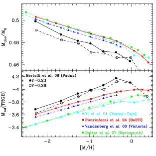
Figure 3: The trends of $M_{core}^{He}$ and $\rm M_{bol}^{TRGB}$ as a function of the metallicity as provided by the most recent stellar model libraries (see text for more details).

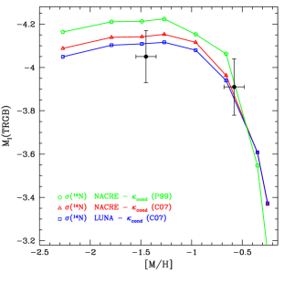
Figure 4: The I-band TRGB magnitude: a comparison among GGCs data and model predictions based on various assumptions on the conductive opacity and/or an updated ${}^{14}N(p,\gamma)^{15}O$ reaction rate.

We show in fig. 4 the comparison of the most recent results (Bertelli et al. 2008 - Padua, Pietrinferni et al. 2004 - BaSTI, Vandenberg et al. 2000 - Victoria, Dotter et al. 2007 - Dartmouth, Yi et al. 2001 - Yonsei-Yale) concerning the TRGB bolometric magnitude and $M_{core}^{He}$ at the He-flash; the displayed quantities refer to a 0.8$M_{\odot}$ model and various initial metallicities. When excluding the Padua models, there exists a fair agreement among the various predictions about $M_{core}^{He}$: at fixed metallicity the spread among the various sets of models is at the level of $0.003M_{\odot}$. For the Padua models, we show the results corresponding to the two different initial He contents adopted by the authors: we have no clear explanation for the fact that the Padua models predict the lowest values for $M_{core}^{He}$, as well as for the presence of an ‘erratic’ behavior of the values corresponding to the different He abundances: for a fixed total mass and metallicity, the $M_{core}^{He}$ value is expected to be a monotonic function of the initial He abundance. Concerning the trend of $\rm M_{bol}^{\rm TRGB}$, all model predictions at a given metallicity are in agreement within $\sim 0.15$ mag, with the exception of the Padua models that appear to be brighter, at odds with the fact that they predict the lowest $M_{core}^{He}$ values. In case of the Yonsei-Yale models, the result is also surprising since the fainter TRGB luminosity cannot be explained by much smaller $M_{core}^{He}$ values, because this quantity is very similar to, for instance, the results given by VandenBerg et al. (2000). When neglecting the Padua and Yonsei-Yale models, the $\sim 0.1$ mag spread among the different TRGB brightness estimates can be interpreted in terms of differences in the adopted physical inputs.

Due to its relevance as standard candle, it is worthwhile showing a comparison between theoretical predictions about the I-Cousins magnitude of the TRGB and empirical data. This comparison is displayed in fig. 4, where we show the data for the GGCs $\omega$ Cen. and 47 Tuc (Bellazzini et al., 2004), and theoretical calibrations of $M_{I}^{TRGB}$ as a function of the metallicity based on our own stellar models by using various assumptions concerning the conductive opacity and the rate for the nuclear reaction ${}^{14}N(p,\gamma)^{15}O$ (see Pietrinferni et al., 2010, for details). The calibrations based on the most updated physics are in fine agreement with the empirical evidence.

4 Conclusions

We have shown that theoretical predictions on stellar models are affected by sizeable uncertainties, a clear proof being the occurrence of not-negligible differences between results provided by different theoretical groups. From the point of view of stellar models users, the best approach to be used for properly accounting for these uncertainties, is to not use evolutionary results with an uncritical approach and, also to adopt as many as possible independent theoretical predictions in order to have an idea of the uncertainty existing in the match between theory and observations.

On the other hand, stellar model makers should continue their effort of continuously updating their models in order to account for the ‘best’ physics available at any time, and consider the various empirical constraints as a benchmark of their stellar models. This represents a fundamental step for obtaining as much as possible accurate and reliable stellar models.