Second–order hyperbolic Fuchsian systems.
Asymptotic behavior of geodesics in Gowdy spacetimes

Abstract

Recent work by the authors led to the development of a mathematical theory dealing with ‘second–order hyperbolic Fuchsian systems’, as we call them. In the present paper, we adopt a physical standpoint and discuss the implications of this theory which provides one with a new tool to tackle the Einstein equations of general relativity (under certain symmetry assumptions). Specifically, we formulate the ‘Fuchsian singular initial value problem’ and apply our general analysis to the broad class of vacuum Gowdy spacetimes with spatial toroidal topology. Our main focus is on providing a detailed description of the asymptotic geometry near the initial singularity of these inhomogeneous cosmological spacetimes and, especially, analyzing the asymptotic behavior of timelike geodesics —which represent the trajectories of freely falling observers — and null geodesics. In particular, we numerically construct Gowdy spacetimes which contain a black hole–like region together with a flat Minkowski–like region. By using the Fuchsian technique, we investigate the effect of the gravitational interaction between these two regions and we study the unexpected behavior of geodesic trajectories within the intermediate part of the spacetime limited by these two regions.

I Introduction

Recent work by the authors beyer10:Fuchsian12 ; beyer10:Fuchsian1 ; beyer10:Fuchsian2 building on earlier and pioneering investigations Kichenassamy97 ; Rendall00 ; isenberg99 ; Choquet-Bruhat05 ; KichenassamyBook ; Choquet08 led to a mathematical theory of the so-called second-order hyperbolic Fuchsian systems. From a physical standpoint, suppose that we have a system of evolution equations that describes the dynamics of some physical configuration. As it is often the case in practice, one is not able to find exact analytical solutions of these equations and, instead, one seeks a description of the dynamics in certain asymptotic regimes of interest. Such an effective description is often found by neglecting certain terms in the evolution equations which, according to physical intuition or other formal arguments, turn out to be inessential. In many applications, this leading-order behavior leads one to a singular problem.

In such a context, the second-order hyperbolic Fuchsian theory, discussed in the present paper, allows one to address the following issues. First of all, it gives precise conditions on the data and the equations whether the leading-order description above is actually consistent with the evolution equations in a well-defined sense and, hence, whether the intuitive or heuristic understanding of the physical system can be validated. It allows us to formulate a singular initial value problem based on this leading-order description and, most importantly in the physical applications, to actually compute approximations of arbitrary accuracy of general solutions of the evolution equations beyond the leading-order description. This singular initial value problem is analogous to the (standard) initial value problem classically formulated for nonlinear hyperbolic equations. The leading-order expansion plays the role of the free Cauchy data and is hence referred to as asymptotic data. We thus construct solutions to the equations which have a prescribed singular behavior. Specifically, keeping in mind our objective to provide suitable tools for the physical applications, we discuss two relevant approximation schemes in the present work which are useful for different purposes. On one hand, the approximation scheme introduced in beyer10:Fuchsian12 (cf. also the earlier work ABL2009 ) can be used to compute numerical solutions of arbitrary accuracy and, therefore, is useful for quantitative statements. On the other hand, another important approximation method can be used to generate formal expansions of arbitrary order and therefore provides a useful tool for qualitative studies, see also Rendall00 .

The proposed theory (together with some forthcoming generalizations, see e.g. beyer:T2symm ) has been found to apply to a variety of problems arising in physics and, especially, in general relativity. In earlier work, we considered Gowdy spacetimes with spatial toroidal topology and we applied the theory to the construction of the so-called asymptotically velocity dominated solutions Eardley71 ; Isenberg89 of the Gowdy equations Gowdy73 ; Berger93 ; Berger97 . In the present paper, we continue this analysis and seek for a deeper physical understanding of the vicinity of the singularity existing in such spacetimes. In particular, we study the behavior of freely falling observers, i.e. timelike geodesics, and we demonstrate that the Fuchsian method allows us to construct families of such curves which “start” on the singularity at prescribed locations. Furthermore, we describe their leading-order behavior.

We emphasize that the issues discussed in the present paper are motivated by the ongoing and very active research on the dynamics of inhomogeneous cosmologies; the reader is referred to the contributions B3 ; B4 ; B5 ; B6 ; B7 ; B8 for further details.

The paper is organized as follows. In a first part, we begin with a general discussion of the second-order hyperbolic Fuchsian theory and our notion of the singular initial value problem. To this end, we first recall some basic material about the (standard) initial value problem for nonlinear hyperbolic equations. The singular initial value problem is discussed next and the similarities with the (standard) initial value problem are stressed. We list the main conditions which need to be checked in order to validate the proposed formulation. This allows to conclude whether the singular initial value problem is well-posed and, hence, that the proposed leading-order description is consistent with the given equations. Then, we outline the description of the two approximation schemes mentioned earlier in this introduction. In the second part of this paper, we apply the theory to (vacuum) Gowdy spacetimes. We first summarize some now classical properties of such spacetimes, and then move on to the core of the present work, that is, the discussion of the asymptotic behavior of freely falling observers in the vicinity of the singularity. Since the geodesic equation is “only” a system of ordinary differential equations (ODE’s), the discussion there highlights the essential aspects of the Fuchsian techniques without being distracted by the rather technical issues arising for partial differential equations (PDE’s). Our discussion demonstrates how the theory can be applied, how the singular initial value problem works, and what limitations should be kept in mind in the applications. We complete this second part of the paper with extensive numerical experiments leading to the construction of Gowdy spacetimes with Cauchy horizons. The paper closes with a concluding section.

II Second-order hyperbolic Fuchsian equations

II.1 The initial value problem

Recall that the function $u(t,x)$ describing the displacement from an equilibrium position $u(t,x)=0$ of a (violin, say) string satisfies the linear wave equation

$$\Box u:=\frac{\partial^{2}u}{\partial t^{2}}-c^{2}\frac{\partial^{2}u}{\partial x^{2}}=0,$$ (1)

in which $c$ represents the speed of sound, $t$ is the time variable, and the spatial variable $x$ varies in some interval. This equation will serve as a model equation in all of the following discussion; recall that, in particular, Einstein’s field equations imply, in certain gauges, nonlinear wave equations which describe the dynamics of the gravitational field Friedrich85 ; Alcubierre:Book . Before we focus on such wave-type equations, let us, however, study some of the principles of the simple linear model Eq. (1) first. The initial value problem associated with the wave equation is posed as follows. If we choose (smooth, say) free data functions denoted here by $u_{*}(x)$ and $u_{**}(x)$, then there exists precisely one (smooth) solution $u(t,x)$ of the wave equation (1) with the property that

$$u(0,x)=u_{*}(x)\quad\text{and}\quad\partial_{t}u(0,x)=u_{**}(x).$$

The initial value problem associated with the wave equation is hence well-posed, as we will say. The interpretation of the well-posedness of the initial value problem for the wave equation is as follows. Since the state of the string at the initial time uniquely determines the state of the string at all times, the physical theory describing the evolution of string via the wave equation is deterministic. Indeed, the mathematical notion of well-posedness of the initial value problem is strongly related to the physical notion of determinism and is hence a concept of fundamental importance.

Note that we are ignoring here the issue of the formulation of the boundary conditions and, throughout this paper and without further notice, simplify the discussion by assuming periodicity in space. Moreover, note that one can write the solutions of the wave equation explicitly in terms of the data functions $u_{*}$ and $u_{**}$. We will not make use of this since, later, we will in fact be interested in general nonlinear equations for which no explicit solution formulas are known in general.

Let us discuss the following important interpretation of the initial value problem for the wave equation. For this consider the Taylor expansion in $t$ of the solution at the initial time

$$u(t,x)=u(0,x)+\partial_{t}u(0,x)t+\frac{1}{2}\partial^{2}_{t}u(0,x)t^{2}+\ldots$$

The first two terms are determined by the data. All higher-order terms, however, are determined by the wave equation from the initial data, as demonstrated by the expansion

$$\begin{split}u(t,x)=\,&u_{*}(x)+u_{**}(x)t\\ &+\frac{1}{2}c^{2}u_{*}^{\prime\prime}(x)t^{2}+\frac{1}{6}c^{2}u_{**}^{\prime\prime}(x)t^{3}+\ldots.\end{split}$$ (2)

Hence, the initial value problem for the wave equation allows us to fix freely the short-time behavior of the solutions, i.e. the time for which $t\ll 1$ when terms of order $t^{2}$ etc. are negligible. However, this means that the solution is fixed for all times, and in particular we are not able to control the long-time behavior in addition.

This just observed fundamental phenomenology for the simple wave equation carries over to a much larger class of equations, namely to general hyperbolic systems , also referred to as nonlinear wave equations. We will not give a formal definition here, cf. Alcubierre:Book ; for the purpose of this paper we can mostly think of equations of the form Eq. (1) with certain nonlinearities. Particular examples will be given later. The main fact is that the initial value problem is well-posed in the same way as it is for Eq. (1). In particular, the short-term behavior of solutions can be prescribed directly by means of free data functions, while the equation, as soon as the data have been prescribed, leaves no further freedom to influence the long-time behavior.

We note that solutions of general nonlinear hyperbolic equations often show severe phenomena which occur after “longer” evolution times, for example blow up of solutions, shocks, loss of uniqueness and bifurcations, etc. These nonlinear phenomena are extremely important for many applications in modern physics and mathematics. The questions how and under which conditions those develop from smooth initial conditions is often particularly challenging.

A key result in general relativity is that Einstein’s vacuum field equations imply a system of (very complicated) nonlinear wave equations plus constraint equations. The associated initial value problem is well-posed. However, its formulation is more involved than the one met with a standard system of hyperbolic equations. On one hand, Einstein equations are geometric equations in nature and, consequently, the type and character of the resulting partial differential equations depend crucially on the choice of the coordinate gauge and the chosen formulation. On the other hand, Einstein equations do not lead to a standard initial value problem due to the presence of constraints. Thanks to the fact that the constraints propagate, the essential properties of the initial value problem are, however, preserved. Indeed, the well-posedness of the initial value problem for the Einstein equations was established first, in 1952, by Choquet–Bruhat choquet52 .

II.2 The singular initial value problem

As already pointed out in the introduction of this paper, many physical applications give rise to an effective leading-order description at some initial time, say $t=0$, which is singular in nature. It is thus desirable to seek for a formulation of the initial value problem when leading-order terms, that are more general than the truncated Taylor expansions Eq. (2), are prescribed. One may wonder whether it is possible to formulate such a singular initial value problem, for which we are allowed to prescribe the behavior at the vicinity of the singularity, at least for short times, in the same way as the (standard) initial value problem allows us to fix the behavior close to the “regular” initial time. Whenever this is possible, such a theory gives us the opportunity, for example, to study “how smooth conditions arise from singularities”, as opposed to “how singularities develop from smooth conditions” as is usually done with the (standard) initial value problem.

Let us, however, mention the following difficulty first. It is not reasonable to expect that a singular initial value problem as above is well-defined for general equations, except possibly in the physically uninteresting set-up of analytic data and solutions. In practice, attention are concentrated to equations of a particular type and, specifically, we focus here on the class of second–order hyperbolic Fuchsian PDE’s introduced in beyer10:Fuchsian12 , that is,

$$\begin{split}&u_{tt}(t,x)+\frac{2a(x)+1}{t}u_{t}(t,x)+\frac{b(x)}{t^{2}}u(t,x)\\ &=t^{-2}f(t,x,u,u_{x},u_{t})+c^{2}(t,x)u_{xx}(t,x).\end{split}$$ (3)

See beyer:T2symm for the generalization to quasilinear hyperbolic equations. For simplicity, let us suppose for all of what follows that the spatial domain is one-dimensional and that all functions under consideration are periodic in the spatial variable $x$. The vector-valued map $u$ is the unknown in (3), while the given matrix-valued coefficients $a,b,c$ are assumed to be smooth and, for the sake of simplicity in this paper, diagonal. The source–term $f$ is the nonlinearity and will be required later to satisfy a certain “decay condition”. This latter condition will imply that the terms on the left-hand side impose the leading–order behavior in $t$. In short, second–order hyperbolic Fuchsian PDE’s are systems of hyperbolic equations containing singular coefficients at $t=0$. We are interested in general solutions defined for $t>0$ and in their asymptotic behavior for $t\rightarrow 0+$.

The following presentation will become more transparent if we now multiply Eq. (3) by the factor $t^{2}$ (which vanishes on the singularity) and we introduce the singular operator $D=t\partial_{t}$, so that

$$\begin{split}D^{2}u(t,x)+2a(x)Du(t,x)+b(x)u(t,x)\\ =f(t,x,u,tu_{x},Du)+t^{2}c^{2}(t,x)u_{xx}(t,x).\end{split}$$ (4)

Let us emphasize that $D^{2}u$ stands for $t\partial_{t}(t\partial_{t}u)$. The left–hand side of the above equation is referred to as the Fuchsian principal part, while the right–hand side is referred to as the Fuchsian source-term. Let us also introduce the associated operator

$$\begin{split}L[u]:=&D^{2}u(t,x)+2a(x)Du(t,x)+b(x)u(t,x)\\ &-t^{2}c^{2}(t,x)u_{xx}(t,x).\end{split}$$ (5)

Now, in order to formulate the singular initial value problem we look for solutions $u$ of the form

$$u=u_{0}+w,$$

where the remainder $w$ must be of “higher order” (in $t$ and at $t=0$) than the leading–order term $u_{0}$. This will be described in more details below; see also beyer10:Fuchsian12 for precise mathematical statements. Provided, for a given $u_{0}$, a unique remainder $w$ exists, which is smooth for all $t>0$, such that $u$ is a solution, then the singular initial value problem associated with $u_{0}$ will be called well-posed. The function $u_{0}$ plays the role of the (in general) “singular data” and should be a prescribed smooth function which is defined for all $t>0$ but can be singular when $t\rightarrow 0$.

As we will see, only certain well-chosen functions $u_{0}$ will be compatible with the given system of equations. To determine the class of compatible leading-order terms for a given equation, a “guess” $u_{0}$ must be made in a first step as mentioned before, often on the basis of physical or heuristical arguments. In a second step, certain conditions need to be checked in order to determine whether the chosen function $u_{0}$ is compatible with the equation in the sense that it gives rise to a well-posed singular initial value problem. In order to understand what this means, let us return to the example of the wave equation Eq. (1) which is of second-order hyperbolic Fuchsian form Eq. (3), with here $a=-1/2$, $b=0$, $c=1$ and $f=0$. The requirement that the solution $u$ is smooth for $t>0$ implies that $u_{0}$ must be smooth in the limit $t\rightarrow 0$ and hence the leading-order term $u_{0}$ is only compatible with the equation if it is of the form of a (truncated) Taylor expansion as in Eq. (2). In other words, since there are no smooth solutions of the wave equation which become singular in the limit $t\rightarrow 0$, the leading-order term must be of this form. Note that if this $u_{0}$ consists of the first two terms of the Taylor expansion for example, then the remainder is $O(t^{2})$, i.e. of higher order than $u_{0}$. A particular consequence of this is that the standard initial value problem of the wave equation is just a special case of a singular initial value problem.

In order to determine $u_{0}$ beyond the case of the standard wave equation, we will now treat the following “canonical set-up” which will turn out to be directly useful later in this paper. Although the following conditions are not always satisfied in the later discussion directly, we will be able to reduce our problems below to this canonical case. To this end, let us make the basic assumption that the right–hand side of Eq. (3), i.e. both the source-term function $f$ and the second-order spatial derivative term, are negligible at $t=0$ in the sense that the leading-order behavior of the solutions to the full equation is driven by its principal part, only, in the now to be discussed sense. For instance, in general relativity and the Einstein’s vacuum field equations, the famous BKL conjecture lifshitz63 ; belinskii70 ; belinskii82 ; Rendall05 claims that for large parts of the dynamics close to generic singularities, the kinetic terms in Einstein’s field equations dominate the potential terms. If the singularity is asymptotically velocity dominated, see above, then this is a good description all the way to the singularity, and therefore our working assumption, where in particular all spatial derivatives are assumed to be negligible at $t=0$, is relevant. Indeed Fuchsian techniques, under certain analyticity assumptions, have been applied to asymptotically velocity dominated spacetimes before even beyond the Gowdy case isenberg99 ; Andersson00 ; Damour2002 ; Choquet-Bruhat05 ; Heinzle2011 . In the general case predicted by the BKL conjecture, however, potential terms can lead to bounces from one kinetically dominated epoch to another and hence are not always negligible. As far as we know, Fuchsian techniques have not been applied to such “Mixmaster-like” singularities yet, and it is not clear whether this is possible.

In any case, let us now go as far as choosing the leading-order term $u_{0}$ for the singular initial value problem to be a solution of the system of ordinary differential equations (in which now $x$ plays the role of a parameter) obtained from Eq. (3) by setting the right–hand side to zero. Since the coefficients of this ODE’s do not depend on $t$, we can find explicit solutions easily as follows:

$$u_{0}=\begin{cases}u_{*}(x)\,t^{-a(x)}\log t+u_{**}(x)\,t^{-a(x)},&a^{2}=b,\\ u_{*}(x)\,t^{-\lambda_{1}(x)}+u_{**}(x)\,t^{-\lambda_{2}(x)},&a^{2}\neq b.\end{cases}$$ (6)

Here, the smooth asymptotic data $u_{*}$ and $u_{**}$ can be freely specified, and we have set

$$\lambda_{1}:=a+\sqrt{a^{2}-b},\quad\lambda_{2}:=a-\sqrt{a^{2}-b}.$$

Note for later purposes that, for such a canonical two-term expansion, one has

$$L[u_{0}]=-t^{2}c^{2}\partial_{x}^{2}u_{0}.$$

By convention, we impose that $\Re\lambda_{1}\geq\Re\lambda_{2}$, where $\Re$ denotes the real part of a complex number. We refer to this leading-order term $u_{0}$ as the canonical two-term expansion and the underlying argument used to derive it as the Fuchsian heuristics; this is motivated by the fact that $u_{0}$ is determined by Fuchsian ordinary differential equations. The singular initial value problem based on this leading-order term will be referred to as the standard singular initial value problem. For given asymptotic data, this problem is well-posed if there exists a unique remainder $w$ which is of order $O(t^{\alpha})$ with $\alpha>-\Re\lambda_{2}$ at $t=0$ and is smooth for $t>0$.

The question, whether the canonical two-term expansion above, or any other choice of leading–order term, is compatible with the given equations and gives rise to a well–posed singular initial value problem, depends strongly on properties of the right-hand side of the equations. We cannot go into the mathematical details here and refer the reader to beyer10:Fuchsian12 . The most important condition is the following one. Consider the class of functions $u=u_{0}+w$ associated with a fixed leading–order function $u_{0}$ and with all functions $w$ that are smooth for $t>0$ and (together with all of their derivatives) are of order $O(t^{\alpha})$ at $t=0$ for a fixed spatially-dependent function $\alpha$. Here, it is required that $\alpha$ is sufficiently large so that $w$ can be indeed treated as “higher order” in $t$. Now, provided the source–term $f$ maps each such function to a function which is smooth for all $t>0$ and is (including all derivatives) of higher order, say $O(t^{\alpha+\epsilon})$ for some arbitrarily small $\epsilon$, and provided the function $L[u_{0}]$ is thus of order $O(t^{\alpha+\epsilon})$, then the singular initial value problem can be proven to be well–posed. More precisely, this latter condition is sufficient for well-posedness in the case of Fuchsian ODE’s systems, only, i.e. when the right-hand side contains no spatial derivatives beyer10:Fuchsian1 . In the PDE’s set-up, there are further restrictions, in particular on the coefficients of the principal part, which we will, however, not discuss here; again see beyer10:Fuchsian12 for details.

As we will discuss later, the leading-order term function $u_{0}$ does not necessarily consist of only two terms as in Eq. (6). However, the free asymptotic data will in general consist of two free functions, at least for the class of second–order hyperbolic equations under consideration here.

As an example, consider the Euler-Poisson-Darboux equation which also plays a role in general relativity; for example, the Gowdy equations discussed later (see Eq. (11), below) reduce to such an equation (in the so-called polarized case $Q=0$, see below). For any real positive constant $\kappa$, let

$$u_{tt}-\frac{\kappa-1}{t}u_{t}=u_{xx}.$$ (7)

This is a linear second-order hyperbolic Fuchsian equation containing a single singular term. The canonical two-term expansion in this case reads

$$u_{0}(t,x)=\begin{cases}u_{*}(x)+u_{**}(x)t^{\kappa},&\kappa>0,\\ u_{*}(x)\log t+u_{**}(x),&\kappa=0.\end{cases}$$

In beyer10:Fuchsian12 we showed that the singular initial value problem is well-posed if and only if $\kappa<2$. On the other hand the second–order spatial derivative term is of order $O(t^{2})$ when $\kappa\geq 2$, and is therefore not negligible at $t=0$. Note that the (standard) initial value problem for the wave equation Eq. (1) is recovered in the special case $\kappa=1$ (and for $c=1$).

II.3 Approximate solutions with arbitrary accuracy

The well-posedness theory would not be complete without means to actually compute the solutions under consideration. Our approximation scheme in beyer10:Fuchsian12 precisely allows to compute general solutions to the singular initial value problem (when they exist) with arbitrary accuracy and can easily be implemented in practice.

We suppose that a second–order hyperbolic Fuchsian system of the form Eq. (3) together with a leading–order term $u_{0}$ are given, the latter being not necessarily of the canonical form Eq. (6). Note that Eq. (3), being a hyperbolic system, gives rise to a well-posed (standard) initial value problem with data prescribed at any time $t>0$. This fact, together with the fact that the solution is presumably described accurately by $u_{0}$ for small $t>0$, can be exploited to approximate the solution of the singular initial value problem as follows; the idea is also illustrated in Fig. 1, where we plot the solution $u$ and the leading-order term $u_{0}$ schematically (as well as other functions to be described now).

Observe in the figure that the leading-order function $u_{0}$ deviates from the solution $u$ for larger $t$. However, we can choose a small time $t_{1}>0$ and use the values $u_{0}$ and $\partial_{t}u_{0}$ at $t_{1}$ as data for the (standard) initial value problem associated with Eq. (3). We solve this initial value problem to the future of $t_{1}$ and get a function labeled by “approximation $t_{1}$” in the plot. Since it is a solution of the equation which is close to the actual solution $u$ at $t_{1}$, it will be close to $u$ at least on some short time interval. Now, the choice of $t_{1}$ above was arbitrary, and in a next step we can pick some other time $t_{2}$ between $0$ and $t_{1}$ and go through the same procedure. The resulting function labeled by “approximation $t_{2}$” in the plot can be expected to be a better approximation of $u$ than the previous function, since the deviation from $u$ at $t_{2}$ is smaller. Eventually, we construct a whole sequence of approximate solutions with initial times $t_{n}\rightarrow 0$. If the procedure works then this sequence approaches the actual solution to the singular initial value problem. The errors become smaller the smaller the initial time is. In fact, our well-posedness theory in beyer10:Fuchsian12 makes use precisely of this approximation scheme for the existence proof. Therein, we proved convergence and also provided explicit error estimates. This scheme can be implemented numerically without difficulty, since it requires to compute a sequence of solutions to the (standard) initial value problem for hyperbolic equations, for which a variety of robust and efficient schemes are available in the literature Kreiss ; LeVeque .

Figure 1: Illustration of the approximation scheme.

Let us make some comments about our actual numerical implementation of the above scheme; more details can be found in beyer10:Fuchsian12 ; beyer10:Fuchsian2 . First of all, recall that in order to compute an approximate solution in the sense above, we must solve Eq. (3) with initial data at some $t_{0}>0$ toward the future direction $t\geq t_{0}$. Moreover, we have to be able to choose $t_{0}$ as small as needed in order to get an approximation as accurate as possible. The main obstacles here are the factors $1/t$ or $1/t^{2}$ in the hyperbolic equation. We address this issue by introducing a new time coordinate

$$\tau:=\log t.$$

For instance, under this transformation, the Euler–Poisson–Darboux Eq. (7) becomes

$$\partial_{\tau}^{2}u-\kappa\,\partial_{\tau}u-e^{2\tau}\partial_{x}^{2}u=0.$$

With this coordinate choice, we have achieved that there is no singular term in this equation; the main price to pay, however, is that the singularity $t=0$ has been “shifted to” $\tau=-\infty$. Another disadvantage is that the characteristic speed of this equation (defined with respect to the $\tau$-coordinate) is $e^{\tau}$ and hence increases exponentially in time. For any explicit discretization scheme, we can thus expect that the so-called CFL condition is always violated after some time on. But we do not expect that this is a genuine problem in practice. The new time coordinate is only introduced to deal with very small times $t$. From any given larger time on, we could, if necessary, switch back to the original time coordinate $t$ so that the CFL restriction above disappears. All the numerical solutions presented in this paper, however, were done exclusively using the time coordinate $\tau$.

In our numerical code, we assume that a leading-order term $u_{0}$ has been fixed and, then, we write the equation in terms of the remainder $w$. The initial data, which we need to prescribe for each approximate solution at initial time $\tau_{0}$ is hence

$$w(\tau_{0},x)=0,\quad\partial_{\tau}w(\tau_{0},x)=0.$$

Inspired by Kreiss et al. Kreiss2002 and by the general idea of the method of lines Kreiss , we discretize the equation with second–order finite–differencing operators.

II.4 Canonical expansions of arbitrarily high order

One final tool remains to be presented here, that is, another approach to analyze the behavior of solutions beyond the leading order. Consider the standard singular initial value problem associated with Eq. (4) together with the canonical two–term expansion Eq. (6). Let us suppose that it is well-posed, i.e. for this given $u_{0}$, there exists a unique solution $u=u_{0}+w$ with remainder $w$ which is smooth for $t>0$ and behaves like $O(t^{\alpha})$ for some sufficiently large $\alpha$.

Consider first the ODE’s case of Eq. (4), i.e.

$$D^{2}v(t,x)+2a(x)Dv(t,x)+b(x)v(t,x)=f_{0}(t,x),$$

where $x$ is now regarded as a parameter and $f_{0}(t,x)$ is a given function and is smooth for $t>0$. As discussed before, there exists a unique solution $v=u_{0}+\tilde{w}$ of this equation, provided suitable assumptions on $f_{0}$ are made at $t=0$. At any given spatial point $x$, define

$$(H[f_{0}])(t,x):=t^{-a(x)}\int_{0}^{t}f_{0}(s,x)s^{a(x)-1}\ln\frac{t}{s}\,ds,$$

if $a^{2}(x)^{2}=b(x)$, and

$$(H[f_{0}])(t,x):= \frac{t^{-\lambda_{2}(x)}}{\lambda_{1}(x)-\lambda_{2}(x)}\int_{0}^{t}f_{0}(s,x)s^{\lambda_{2}(x)-1}ds$$

$$-\frac{t^{-\lambda_{1}(x)}}{\lambda_{1}(x)-\lambda_{2}(x)}\int_{0}^{t}f_{0}(s,x)s^{\lambda_{1}(x)-1},$$

if $a^{2}(x)\not=b(x)$. Then, if these integrals converge, it can be checked that the solution of the singular initial value problem is given by

$$v=u_{0}+H[f_{0}].$$ (8)

Next, consider the following ordinary Fuchsian differential equation

$$\begin{split}&D^{2}v(t,x)+2a(x)Dv(t,x)+b(x)v(t,x)\\ &=f(t,x,u,tu_{x},Du)+t^{2}c^{2}(t,x)u_{xx}(t,x),\end{split}$$ (9)

which follows from Eq. (4) for some given $u=u_{0}+\widehat{w}$ where $\widehat{w}$ is the remainder of $u$ in the same sense as above. Here $v$ is the new unknown. Under the conditions before, the singular initial value problem with leading-order term $u_{0}$ associated with this equation for $v$ is well-posed and there exists a unique solution.

Now suppose that we start with a seed function $u=u_{0}$. Then the singular initial value problem for Eq. (9) associated with the leading–order term $u_{0}$ determines a unique function $v$, which we call $u_{1}$. Then we use this function $u_{1}$ instead of $u$ in the right–hand side of Eq. (9) and, consequently, determine a new approximate solution $v$ to the singular initial value problem associated with Eq. (9), which we call $u_{2}$. Continuing inductively, we determine a sequence of functions $(u_{n})$, each of these being computed using the integral expressions above and having $u_{0}$ as their leading-order term. It was observed in Kichenassamy97 ; Rendall00 ; beyer10:Fuchsian1 that $u_{j+1}-u_{j}$ is $O(t^{\beta_{j}})$ at $t=0$ with $(\beta_{j})$ some monotonically increasing sequence of constants. Hence $u_{j}$ can be interpreted as a formal expansion of the solution at $t=0$ whose order in $t$ increases with $j$. Moreover, it turns out that the residual, which is obtained when $u_{j}$ is plugged into the full equation Eq. (4), behaves like a positive power in $t$ at $t=0$ which increases with $j$.

We note that one can find conditions for which this sequence $(u_{n})$ actually converges to the solution of the singular initial value problem in general only in the case of Fuchsian ordinary differential equations. In the PDE’s case, the sequence $(u_{n})$ does not converge in general. Even though it may not converge, it is still useful for a qualitative study of general solutions. If one is rather interested in quantitative statements and in actual convergence, then the approximation procedure in the previous subsection must be used.

III Geodesics in Gowdy spacetimes

III.1 Background material

Before we apply the general theory, we provide some background material about Gowdy spacetimes. These are spacetimes with two commuting spatial Killing vector fields, for which one can thus introduce coordinates $(t,x,y,z)$ so that the functions $y,z$ are aligned with the symmetries. The so-called Gowdy metric can then be written in the form

$$\begin{split}g=\,&\frac{1}{\sqrt{t}}\,e^{\Lambda/2}(-dt^{2}+dx^{2})\\ &+t\,\big{(}e^{P}(dy+Qdz)^{2}+e^{-P}dz\big{)},\end{split}$$ (10)

with $t>0$. It therefore depends on three coefficients $P=P(t,x)$, $Q=Q(t,x)$, and $\Lambda=\Lambda(t,x)$. We assume that these functions are periodic with respect to $x$. Clearly, the metric is singular (in some sense) at $t=0$. We recall that a Gowdy metric is said to be polarized if the function $Q$ vanishes.

Einstein’s vacuum equations imply the following second–order wave equations for $P,Q$:

$$P_{tt}+\frac{P_{t}}{t}-P_{xx} =e^{2P}(Q^{2}_{t}-Q^{2}_{x}),$$ (11)

$$Q_{tt}+\frac{Q_{t}}{t}-Q_{xx} =-2(P_{t}Q_{t}-P_{x}Q_{x}),$$

which are decoupled from the wave equation satisfied by the third coefficient $\Lambda$:

$$\Lambda_{tt}-\Lambda_{xx}=P_{x}^{2}-P_{t}^{2}+e^{2P}(Q_{x}^{2}-Q_{t}^{2}).$$ (12)

Moreover, the Einstein equations imply the following constraint equations:

$$\begin{split}\Lambda_{x}&=2t\,\big{(}P_{x}P_{t}+e^{2P}Q_{x}Q_{t}\big{)},\\ \Lambda_{t}&=t\,\big{(}P_{x}^{2}+te^{2P}Q_{x}^{2}+P_{t}^{2}+e^{2P}Q_{t}^{2}\big{)}.\end{split}$$ (13)

Eqs. (11) represent the essential set of Einstein’s field equations for Gowdy spacetimes; cf. Berger97 for further details. We refer to them as the Gowdy equations.

Let us now proceed with a heuristic discussion of the equations in order to motivate the choice of the leading-order term for the singular initial value problem. Based on extensive numerical experiments Berger93 ; Berger97 ; Andersson03 and the ideas underlying the (already mentioned) BKL conjecture, it is conjectured that the spatial derivatives of solutions $(P,Q)$ to (11) becomes negligible as one approaches the singularity and, hence, $(P,Q)$ approach a solution of the ordinary differential equations

$$P_{tt}+{P_{t}\over t}=e^{2P}Q^{2}_{t},\quad Q_{tt}+{Q_{t}\over t}=-2\,P_{t}\,Q_{t}.$$

These equations are referred to as the velocity term dominated (VTD) equations. They admit solutions that are given explicitly by

$$\begin{split}P(t,x)&=\log\big{(}\alpha\,t^{k}(1+\zeta^{2}t^{-2k})\big{)},\\ Q(t,x)&=\xi-{\zeta\,t^{-2k}\over\alpha\,(1+\zeta^{2}t^{-2k})},\end{split}$$ (14)

where $x$ plays simply the role of a parameter and ${\alpha>0}$, $\zeta,\xi,k$ are arbitrary $2\pi$-periodic functions of $x$. We assume in the following that $k>0$ and $\zeta\not=0$. Based on the above formulas, it is a simple matter to determine the expansion of the function $P$ near $t=0$, that is,

$$\lim_{t\to 0}{P(t,x)\over\log t}=\lim_{t\to 0}t\,P_{t}(t,x)=-k,$$

and

$$\lim_{t\to 0}\big{(}P(t,x)+k(x)\log t\big{)}=\log(\alpha\zeta^{2}).$$

Similarly, for the function $Q$ we obtain

$$\lim_{t\to 0}Q(t,x)=\xi-\dfrac{1}{\alpha\zeta},$$

$$\lim_{t\to 0}t^{-2k}\,\big{(}Q(t,x)-\xi+\dfrac{1}{\alpha\zeta}\big{)}=\dfrac{1}{\alpha\zeta^{3}}.$$

We thus arrive at the expansions

$$\begin{split}P(t,x)&=-k(x)\log t+P_{**}(x)+\ldots,\\ Q(t,x)&=Q_{*}(x)+t^{2k(x)}Q_{**}(x)+\ldots,\end{split}$$ (15)

in which $k$, $P_{**}$, $Q_{*}$, $Q_{**}$ are functions of $x$. In general, $P$ blows up to $+\infty$ when one approaches the singularity, while $Q$ remains bounded. Note that if the assumption $k>0$ is dropped in Eq. (14), then it turns out that we must substitute $k$ by $|k|$ in most of the previous expressions. In other words, without loss of generality we can assume $k\geq 0$ for the leading-order expansion Eq. (15); we will ignore the exceptional case $k=0$ in most of the following discussion.

It was shown in beyer10:Fuchsian12 that this leading-order term Eq. (15) is the canonical two-term expansion of the Gowdy equations. Indeed, we found that the singular initial value problem is well-posed as long as $k$ is a function with values in the interval $(0,1)$. If $\partial_{x}Q_{*}(x)=0$ at points where $k\geq 1$, then the singular initial value problem is also well-posed. These restrictions are related to the formation of spikes, investigated earlier in Berger93 ; Berger97 ; Andersson03 . For asymptotic data $Q_{*}\equiv Q_{**}\equiv 0$, the corresponding solution is polarized and then the function $k(x)$ may take all values in $\mathbb{R}$. Given a solution of Eq. (11) with a leading-order term Eq. (15) satisfying these restrictions, then also Eq. (12) can be solved as a singular initial value problem with leading-order term

$$\Lambda(t,x)=\Lambda_{*}(x)\log t+\Lambda_{**}(x)+\ldots,$$ (16)

where

$$\begin{split}\Lambda_{*}(x)=\,&k^{2}(x),\\ \Lambda_{**}(x)=\,&\Lambda_{0}+2\int_{0}^{x}\left(-P_{**}^{\prime}+2e^{2P_{**}}Q_{**}Q_{*}^{\prime}\right)k\,d\widetilde{x}.\end{split}$$ (17)

Here, a prime denotes the derivative with respect to $x$. Note that periodicity in space hence implies the following further restriction on the asymptotic data

$$\int_{0}^{2\pi}\left(-P_{**}^{\prime}+2e^{2P_{**}}Q_{**}Q_{*}^{\prime}\right)k\,d\widetilde{x}=0,$$

and the constraints Eqs. (13) are then satisfied for all $t>0$. It was demonstrated in Andersson03 that solutions of the Gowdy equations which have the leading-order behavior as above approach certain Kasner solutions at $t=0$, with in general different parameters along different timelines toward the singularity.

III.2 Timelike and null geodesics in Gowdy spacetimes

Now we know how to construct Gowdy solutions of Einstein’s vacuum field equations with a prescribed asymptotic behavior, and we can assume that such a spacetime is given. We henceforth study freely falling observers and null geodesics in a vicinity of the time $t=0$.

A geodesic curve $\gamma^{\mu}(s)$ is a solution of

$$\frac{d^{2}\gamma^{\mu}}{ds^{2}}(s)+{{\Gamma_{\nu}}^{\mu}}_{\rho}(\gamma(s))\frac{d\gamma^{\nu}}{ds}(s)\frac{d\gamma^{\rho}}{ds}(s)=0,$$

where $s$ is the affine parameter which, in the timelike case, corresponds to the proper time of the observer traveling along the geodesic. The objects ${{\Gamma_{\nu}}^{\mu}}_{\rho}$ are the Christoffel symbols of the Gowdy spacetimes. For the later discussion it will be more convenient to parametrize the geodesics with respect to the coordinate time $t(s)=\gamma^{0}(s)$. Hence from now on we will consider the functions $\gamma^{\rho}$ as functions of $t$ and a dot will denote the derivative with respect to $t$. We will assume future pointing causal geodesics with $dt(s)/ds>0$. The geodesic equation becomes

$${\ddot{\gamma}^{\mu}}+\left({{\Gamma_{\nu}}^{\mu}}_{\rho}-{{\Gamma_{\nu}}^{0}}_{\rho}\dot{\gamma}^{\mu}\right)\dot{\gamma}^{\nu}\dot{\gamma}^{\rho}=0,$$ (18)

and our main aim in the following is to study the singular initial value problem for this equation. Since it is a system of ODE’s, the analysis in the part of this paper simplifies.

Note that if $\gamma^{\mu}(t)$ is a solution of Eq. (18) we can return to using the affine parameter $s(t)$, determined from the equation

$$-\text{const}=\left(\frac{dt}{ds}\right)^{2}(g_{00}+g_{\alpha\beta}{\dot{\gamma}^{\alpha}}{\dot{\gamma}^{\beta}}),$$ (19)

where $\alpha,\beta=1,2,3$ are the spatial coordinate indices of the metric $g_{\mu\nu}$ of the form Eq. (10). The constant in this equation is positive for a timelike geodesic and zero for a null geodesic, and may be specified freely.

III.3 Orthogonal causal geodesics

Our strategy will be to increase the level of complexity of our problems systematically step by step. We start by discussing causal geodesics which are orthogonal to the Gowdy symmetry orbits, i.e. $\gamma^{y}\equiv\gamma^{z}\equiv 0$. We refer to those as orthogonal geodesics. We find easily that the conditions ${\dot{\gamma}^{y}}={\dot{\gamma}^{z}}=0$ at some initial time $t>0$ implies $\gamma^{y},\gamma^{z}\equiv 0$ for all $t>0$. We write $x(t)$ instead of $\gamma^{x}(t)$ for the only remaining non-trivial component, and the geodesic equation (18) reduces to

$$\begin{split}&\ddot{x}(t)+\frac{t\partial_{t}\Lambda(t,x(t))-1}{4t}\,\big{(}\dot{x}(t)-\dot{x}^{3}(t)\big{)}\\ &-\frac{1}{4}\partial_{x}\Lambda(t,x(t))\,\dot{x}^{2}(t)+\frac{1}{4}\partial_{x}\Lambda(t,x(t))=0.\end{split}$$ (20)

We now study Eq. (20) as a singular initial value problem. The first step is to “guess” the leading-order behavior of the geodesics at $t=0$. Recall that the Gowdy solutions considered above have the property that spatial inhomogeneities close to $t=0$ are insignificant. This suggests that geodesics should behave, to leading order, like in spatially homogeneous (Bianchi I) spacetimes. We will find in the course of the discussion that this does lead to the correct leading-order term for the geodesics in the general Gowdy case.

Step 1. Geodesics in Kasner spacetimes.

Kasner spacetimes are particular spatially homogeneous solutions of the Einstein’s vacuum field equations Wainwright . The Kasner metric can be brought to the Gowdy form Eq. (10) by requiring that

$$\begin{split}P(t,x)&=-k\log t+P_{**},\quad Q(t,x)=0,\\ \Lambda(t,x)&=k^{2}\log t+\Lambda_{**},\end{split}$$ (21)

where $k$, $P_{**}$ and $\Lambda_{**}$ are arbitrary real constants. Hence Kasner solutions can be considered as solutions to the singular initial value problem for the Gowdy equations above with asymptotic data constants $k$, $P_{**}$, $\Lambda_{**}$, cf. Eq. (17). Note that $k$ is allowed to be any value in $\mathbb{R}$ here. Moreover, the constants $P_{**}$ and $\Lambda_{**}$ can be transformed to zero by suitable coordinate transformations. We thus have

$$g=t^{\frac{k^{2}-1}{2}}\big{(}-dt^{2}+dx^{2}\big{)}+t^{1-k}dy^{2}+t^{1+k}dz^{2}$$

and, in the notation made in Wainwright for the Kasner exponents,

$$p_{1} =(k^{2}-1)/(k^{2}+3),$$

$$p_{2} =2(1-k)/(k^{2}+3),$$

$$p_{3} =2(1+k)/(k^{2}+3),$$

so that the three flat Kasner cases are realized by $k=1$, $k=-1$, and $|k|\rightarrow\infty$, respectively.

For any Kasner spacetime, Eq. (20) reduces to

$$\ddot{x}(t)-\frac{1-k^{2}}{4t}\,(\dot{x}(t)-\dot{x}^{3}(t))=0.$$ (22)

This equation can be integrated once

$$\dot{x}(t)=F(\eta(t)):=\frac{x_{1}\eta(t)}{\sqrt{1+x_{1}^{2}\eta^{2}(t)}},$$ (23)

where

$$\eta(t)=t^{\frac{1}{4}(1-k^{2})},$$

and $x_{1}$ is an integration constant. Since $F$ is smooth in $\eta$ for all $\eta\in\mathbb{R}$, we can compute its Taylor expansion at $\eta=0$. If $|k|<1$, this yields the leading-order behavior of $\dot{x}(t)$ at $t=0$. If $|k|>1$, we set $\epsilon:=\eta^{-1}$ and consider the function

$$G(\epsilon):=F(1/\epsilon)=x_{1}\frac{1}{\sqrt{\epsilon^{2}+x_{1}^{2}}},$$

for $\epsilon>0$. This function can be extended as a smooth function to $\epsilon<0$ in only one way and then we are allowed to compute its Taylor expansion at $\epsilon=0$. If $|k|=1$, the exact solution of Eq. (22) is $\dot{x}(t)=const$. Then, after a second integration, the leading terms of the expansions for $x(t)$ at $t=0$ can be computed:

$$x(t)=\begin{cases}x_{0}+\frac{4}{5-k^{2}}x_{1}t^{\frac{1}{4}(5-k^{2})}+\ldots,&|k|<1,\\ x_{0}+\frac{x_{1}}{\sqrt{1+x_{1}^{2}}}t,&|k|=1,\\ \begin{split}x_{0}&+\text{sign}(x_{1})\,t\\ &-\frac{\text{sign}(x_{1})}{x_{1}^{2}(1+k^{2})}t^{\frac{1}{2}(1+k^{2})}+\ldots,\end{split}&|k|>1,\end{cases}$$ (24)

where $x_{0}$ is another integration constant and $x_{1}\not=0$. We have introduced the sign function

$$\text{sign}(x):=\begin{cases}1,&x>0,\\ -1,&x<0.\end{cases}$$

Observe that the case $x_{1}=0$ corresponds to having $x(t)=x_{0}$ for all three cases.

The dots represent terms with $t$-powers $n(1-k^{2})/4+1$ for $n=2,3,\ldots$ in the first case, and $n(k^{2}-1)/2+1$ in the third case. The expression for $|k|=1$ is exact. Given a sequence of Kasner solutions all with, say, $|k|<1$ (and similarly when $|k|>1$) for which $|k|$ approaches $1$, the exponents in the $t$–powers for all of the terms in the infinite series above approach to $1$. The series given by the sum of these terms converges to ${x_{1}}/{\sqrt{1+x_{1}^{2}}}$. This demonstrates the important fact that the closer we choose $|k|$ to the value $1$, the larger all higher–order terms in the series become which, consequently, become no longer negligible.

For all values of $x_{0},x_{1}\in\mathbb{R}$ the orthogonal geodesics above are timelike. Null rays, which are given by $\dot{x}(t)=\pm 1$, are obtained formally in the limit $x_{1}\rightarrow\pm\infty$. Now, Fig. 2 shows the leading-order behavior of orthogonal geodesics close to $t=0$ for the three cases $|k|<1$ and $|k|>1$. In the first case, the geodesics approach a curve at $t=0$ which is at rest with respect to the coordinate system, while in the third case, the geodesics approach a null geodesic. Recall that the case $|k|=1$ corresponds to flat Kasner solutions and hence the curves are straight lines.

Figure 2: Orthogonal geodesics in the homogeneous polarized case for $k=0.5$, $k=1.8$.

Step 2. Fuchsian analysis for the Kasner case.

Instead of deriving Eq. (24) as above, let us now analyze Eq. (22) by means of the Fuchsian heuristics. We multiply Eq. (22) with $t^{2}$ and write the time derivatives by means of the operator $D=t\partial_{t}$:

$$D^{2}x-\frac{1}{4}(5-k^{2})Dx=-\frac{1-k^{2}}{4t^{2}}\,(Dx)^{3}.$$ (25)

This equation is of second-order Fuchsian type. For the standard singular initial value problem for this equation, where we interpret the left-hand side as the principal part and the right–hand side as the source-term, we seek solutions with leading-order behavior

$$x(t)=x_{*}+x_{**}t^{\frac{1}{4}(5-k^{2})}+\ldots,$$ (26)

at $t=0$ for arbitrary prescribed constants $x_{*},x_{**}\in\mathbb{R}$ if $k^{2}<5$. For arbitrary remainders $w=O(t^{\alpha})$ with ${\alpha>\frac{1}{4}(5-k^{2})}$, the source-term is $t^{-2}(Dx)^{3}=O(t^{\frac{3}{4}(5-k^{2})-2})$ in general or identically zero if $|k|=1$. Hence, in general, the source-term is negligible if the following is positive

$$(3(5-k^{2})/4-2)-(5-k^{2})/4=(1-k^{2})/2,$$

since then, the quantity $\alpha$ can be chosen between $(5-k^{2})/4$ and $(3(5-k^{2})/4-2)$ for all derivatives. Therefore the singular initial value problem for Eq. (25) associated with Eq. (26) is well-posed if $|k|<1$. It is certainly also well-posed for $|k|=1$ since then the source-term is identically zero. Indeed, for $|k|\leq 1$, the solutions of the singular initial value problem agree, for appropriate choices of $x_{*}$ and $x_{**}$, with the previous explicit solutions with expansions Eq. (24).

For $|k|>1$, the singular initial value problem for Eq. (25) associated with Eq. (26) is not well-posed, since the source-term is not negligible at $t=0$. Note that Eq. (26) is also not compatible with Eq. (24) in this case. How can we proceed? The expansion Eq. (24) does not have the form of a canonical two-term expansion, due to the additional term $\pm t$. Suppose that the right–hand side of Eq. (25) is not negligible but rather, say, of the same order in $t$ at $t=0$ as the left side. We make the ansatz $x=x_{*}+t^{\beta}c+\ldots$ where $x_{*}$, $\beta$ and $c$ are unknown constants. Then the equation implies that $\beta=1$ and that $c^{2}=1$, independently of $k$. This explains the presence of the term $\pm t$ in Eq. (24). It suggests that we should introduce new variables

$$f_{\pm}(t):=x(t)\mp t,$$ (27)

for the cases $x_{1}>0$ and $x_{1}<0$ in Eq. (24). In terms of those, Eq. (25) reads

$$\begin{split}D^{2}f_{\pm}-\frac{1}{2}(1+k^{2})Df_{\pm}=&\mp\frac{3(1-k^{2})}{4t}\,(Df_{\pm})^{2}\\ &-\frac{1-k^{2}}{4t^{2}}\,(Df_{\pm})^{3}.\end{split}$$ (28)

This is a second-order Fuchsian equation whose canonical two-term expansion is

$$f_{\pm}=x_{*}+t^{\frac{1}{2}(1+k^{2})}x_{**}+\ldots,$$ (29)

at $t=0$ with arbitrary asymptotic data $x_{*},x_{**}\in\mathbb{R}$. This clearly looks promising, cf. Eq. (24). We have to check whether the source-term, i.e. the right–hand side of this equation which consists of two terms is negligible for arbitrary remainders $w=O(t^{\alpha})$ with $\alpha>\frac{1}{2}(1+k^{2})$. For the first term, we get

$$t^{-1}(Df_{\pm})^{2}=O(t^{(1+k^{2})-1}),$$

and hence the following must be positive

$$(1+k^{2})-1-\frac{1}{2}(1+k^{2})=\frac{1}{2}(k^{2}-1).$$

This is true for $|k|>1$. We find that also the second term is negligible for $|k|>1$. Hence the singular initial value problem for Eq. (28) associated with Eq. (29) is well-posed for $|k|>1$. The case $x_{**}=0$ corresponds to null geodesics. We get timelike geodesics if we choose $f_{+}$ for $x_{**}<0$, and, if we choose $f_{-}$ for $x_{**}>0$. The case $x_{1}=0$ before now formally corresponds to the limit $|x_{**}|\rightarrow\infty$.

The leading-order terms for the Fuchsian analysis are therefore consistent with Eq. (24) in the Kasner case. A particular result of our efforts so far is that all causal orthogonal geodesics in Kasner spacetimes have limit points at $t=0$, and hence “start” from points on the singularity which can be prescribed freely. We will see that this is not always the case for non-orthogonal geodesics.

Step 3. The general equation for orthogonal geodesics.

Now we proceed with the singular initial value problem for the general Gowdy inhomogeneous (unpolarized) case for orthogonal causal geodesics. The leading-order behavior which we have identified in the Kasner case before will be taken as the guess for the leading-order behavior here. As before, we consider the function $\Lambda$ as a given solution of Eq. (12) compatible with Eq. (16) and (17) at $t=0$ where, in particular, $k(x)$ is now any given function with the restrictions discussed earlier; we assume here that it is positive. Again, we rewrite Eq. (20) as a second-order Fuchsian equation

$$\begin{split}D^{2}x(t)&-\frac{1}{4}(5-k^{2}(x_{*}))Dx(t)\\ =\,&\frac{1}{4}Dx(t)(k^{2}(x_{*})-D\Lambda(t,x(t)))\\ &-\frac{1-D\Lambda(t,x(t))}{4t^{2}}(Dx(t))^{3}\\ &+\frac{1}{4}((Dx(t))^{2}-t^{2})\partial_{x}\Lambda(t,x(t)).\end{split}$$ (30)

Here, $D\Lambda(t,x(t))$ means the partial derivative of $\Lambda$ with respect to its first argument evaluated at $(t,x(t))$ and multiplied by $t$. Similarly, $\partial_{x}\Lambda(t,x(t))$ means the partial derivative with respect to the second argument evaluated at $(t,x(t))$. Note that we have added the term $k^{2}(x_{*})Dx(t)/4$ to both sides of Eq. (30); the significance of this term for the Fuchsian analysis becomes clear in a moment.

Let us suppose first that $k(x_{*})<1$ for some $x_{*}\in\mathbb{R}$. The additional term $k^{2}(x_{*})Dx(t)/4$ in both sides of the equation has the consequence that the canonical two-term expansion coincides with that of the Kasner case Eq. (24). Hence we shall consider the singular initial value problem associated with the leading-order term

$$x(t)=x_{*}+x_{**}t^{\frac{1}{4}(5-k^{2}(x_{*}))}+\ldots,$$ (31)

for arbitrary $x_{*},x_{**}\in\mathbb{R}$. It follows that the source-term is negligible. In order to show this, we note that

$$k^{2}(x_{*})-D\Lambda(t,x(t))=O(t^{\alpha}),$$

for some $\alpha>0$, and

$$\partial_{x}\Lambda(t,x(t))=O(\log t).$$

Hence, as expected, the singular initial value problem for Eq. (30) associated with Eq. (31) is well-posed if $k(x_{*})<1$. The same conclusion follows directly for $k(x_{*})=1$. In order to study the case $k(x_{*})>1$, we make the same ansatz as in Eq. (27). The resulting equation can be analyzed in exactly the same way in well-posedness can be shown. We omit the details for this case.

So, causal future directed orthogonal geodesics have the asymptotic behavior given by Eq. (24) with $k=k(x_{*})$. Hence we have shown that spatial inhomogeneities as well as the polarization of the given Gowdy spacetime do not play a significant role for the leading-order dynamics of observers close to the singular time $t=0$. Note that Gowdy solutions where $k$ takes values only in the interval $(0,1)$ have a curvature singularity at $t=0$. In particular, this singularity is asymptotically velocity dominated as mentioned before and therefore consistent with the BKL conjecture.

III.4 Non-orthogonal causal geodesics

Next we consider geodesic curves $\gamma^{\mu}(t)$ which are not necessarily orthogonal to the Gowdy group orbits. The full discussion of this problem would, however, be too lengthy for this paper since all three spatial coordinate components of $\gamma^{\mu}$ would then be non–trivial in general. This is why we restrict to the polarized Gowdy case $Q\equiv 0$. In this case, the functions $\gamma^{z}$ and $\gamma^{y}$ decouple in Eq. (18). We assume that $\gamma^{y}\equiv 0$ and $\gamma^{z}$ is non-trivial. There is no loss of generality since one can always switch to the case $\gamma^{z}\equiv 0$ and a non–trivial $\gamma^{y}$ by using the transformation $k\mapsto-k$. The latter mapping just interchanges the two Killing vector fields and, hence, is an isometry of the spacetime. We will be particularly interested in the case $0<|k|<1$, but also in the borderline case $|k|=1$, due to its relevance for the formation of Cauchy horizons, as will be explained below.

As before, we write $x(t)$ and $z(t)$ for the now two non-trivial coordinate components of the geodesic curves. We get the following coupled system of second-order Fuchsian equations

$$\begin{split}D^{2}&x(t)-\frac{1}{4}(5-k^{2}(x_{*}))Dx(t)\\ =&-t^{2}F_{1}(t,x(t))\\ &+F_{2}(t,x(t))Dx(t)+F_{1}(t,x(t))(Dx(t))^{2}\\ &+F_{3}(t,x(t))(Dz(t))^{2}+F_{4}(t,x(t))(Dx(t))^{3}\\ &+F_{5}(t,x(t))(Dz(t))^{2}Dx(t),\\ D^{2}&z(t)-\frac{1}{4}(k^{2}(x_{*})-4k(x_{*})-1)Dz(t)\\ =\,&G_{1}(t,x(t))Dz(t)+G_{2}(t,x(t))Dz(t)Dx(t)\\ &+F_{5}(t,x(t))(Dz(t))^{3}\\ &+F_{4}(t,x(t))Dz(t)(Dx(t))^{2},\end{split}$$ (32)

with

$$\begin{split}F_{1}(t,x)&=\frac{1}{4}\partial_{x}\Lambda(t,x),\\ F_{2}(t,x)&=\frac{1}{4}(k^{2}(x_{*})-D\Lambda(t,x)),\\ F_{3}(t,x)&=-\frac{1}{2}e^{-(P(t,x)+\Lambda(t,x)/2)}t^{3/2}\partial_{x}P(t,x),\\ F_{4}(t,x)&=-\frac{1-D\Lambda(t,x)}{4t^{2}},\\ F_{5}(t,x)&=\frac{1}{2}e^{-(P(t,x)+\Lambda(t,x)/2)}t^{-1/2}(1-DP(t,x)),\end{split}$$

and

$$\begin{split}G_{1}(t,x)&=k(x_{*})+DP(t,x)-\frac{1}{4}\left(k^{2}(x_{*})-D\Lambda(t,x)\right),\\ G_{2}(t,x)&=\partial_{x}P(t,x)+\frac{1}{2}\partial_{x}\Lambda(t,x).\end{split}$$

Note that we have added certain terms to both sides of the equation as before; the second term on the right-hand side of the equation of $x$ would not satisfy the decay condition for well-posedness without the additional term $k^{2}(x_{*})Dx$. The same is true for the additional term $-\frac{1}{4}(k^{2}(x_{*})-4k(x_{*}))Dz$. However, it turns out that the standard singular initial value problem for this system

$$\begin{split}x(t)&=x_{*}+x_{**}t^{\frac{1}{4}(5-k^{2}(x_{*}))}+\ldots,\\ z(t)&=z_{*}+z_{**}t^{\frac{1}{4}(k^{2}(x_{*})-4k(x_{*})-1)}+\ldots,\\ \end{split}$$ (33)

is still not well-posed. Consider for instance the term $F_{5}(t,x(t))(Dz(t))^{3}$ which does not have the correct behavior at $t=0$. This suggests that Eq. (33) is not the correct leading-order behavior. Let us hence step back and think about the dominant physical effects in the same way as we did for the case of orthogonal geodesics.

Step 1. A decoupled equation for $|k|<1$.

We have realized before that inhomogeneities do not contribute to the leading-order term of orthogonal geodesics. This suggests that the Kasner case given by Eq. (21) with constant parameters $k$, $P_{**}$ and $\Lambda_{**}$ is also relevant here. However, it turns out that the standard singular initial value problem remains ill-posed when $|k|\not=1$. Moreover, the system is still too complicated to find explicit solutions and hence we cannot proceed as for instance for Eq. (23).

So let us simplify the equations even more. We can try to neglect the coupling between both equations Eq. (32). For this we consider the equation for $z(t)$ with $x(t)\equiv 0$ (of course the equation for $x$ with vanishing $z$ is the geodesic equation in the orthogonal case already treated):

$$\begin{split}&D^{2}z(t)-\frac{1}{4}(k^{2}-4k-1)Dz(t)\\ &=\frac{1}{2}e^{-(P_{**}+\Lambda_{**}/2)}t^{-(1-k)^{2}/2}(1+k)(Dz(t))^{3}.\end{split}$$ (34)

The standard singular initial value problem is still ill-posed. However, we are able to find explicit solutions for $\dot{z}(t)$, namely

$$\dot{z}(t)=\pm F(\eta(t))t^{-\frac{1}{4}(3-k)(k+1)}\quad\text{or}\quad\dot{z}(t)=0,$$

with

$$F(\eta):=\frac{e^{\frac{3}{4}(P_{**}+\Lambda_{**}/2)}}{\sqrt{e^{\frac{1}{2}(P_{**}+\Lambda_{**}/2)}-2z_{1}\eta}}$$

and

$$\eta(t)=t^{1+k},$$

for arbitrary $z_{1}\in\mathbb{R}$ (provided $\eta$ is sufficiently small). As before, it turns out that $F$ is a smooth function in $\eta$ if $\eta$ is small, and its Taylor expansion at $\eta=0$ henceforth yields an expansion at $t=0$, as long as $k>-1$. After an integration, we then find that

$$z(t)= z_{0}\pm e^{\frac{1}{2}(P_{**}+\Lambda_{**}/2)}\frac{4}{(1-k)^{2}}t^{\frac{1}{4}(1-k)^{2}}$$

$$\pm z_{1}\frac{4}{5+2k+k^{2}}t^{\frac{1}{4}(5+2k+k^{2})}+\ldots,$$

or

$$z(t)=z_{0},$$

both with another free parameter $z_{0}\in\mathbb{R}$. We can see clearly the reason why the standard singular initial value problem Eq. (33) has failed. Namely, this expression is not of the form of a canonical two-term expansion because the second term is of lower order at $t=0$ than the third term if $k>-1$. Similar to the case of orthogonal geodesics, cf. Eqs. (27) and (28), we define

$$f_{\pm}(t):=z(t)\mp e^{\frac{1}{2}(P_{**}+\Lambda_{**}/2)}\frac{4}{(1-k)^{2}}t^{\frac{1}{4}(1-k)^{2}}.$$ (35)

Indeed, this ansatz turns Eq. (34) into a second-order Fuchsian equation for $f_{\pm}$ with a canonical two-term expansion

$$f_{\pm}(t)=z_{*}+z_{**}t^{\frac{1}{4}(5+2k+k^{2})}+\ldots$$

We find easily that the corresponding singular initial value problem is well-posed for $|k|<1$.

Step 2. Kasner case for $|k|<1$.

We have considered Eq. (34), in order to get an insight about the behavior of geodesics. Now we check that the same leading-order term for $z(t)$ as given by Eq. (35) with $f_{\pm}(t)$ defined in Eq. (35) is consistent with the fully coupled set of equation Eqs. (32) for the Kasner case with $|k|<1$. It is important to note that the ansatz Eq. (35) for $z$ does also change the principal part of the equation for $x$ due to terms which have originally been part of the source-term. The equations become

$$D^{2}x(t)-\frac{1}{4}(7+2k-k^{2})Dx(t)=\ldots,$$

$$D^{2}f_{\pm}(t)-\frac{1}{4}(5+2k+k^{2})Df_{\pm}(t)=\ldots,$$

where we do not write the lengthy source-terms. The standard singular initial value problem associated with the leading-order terms

$$x(t) =x_{*}+x_{**}t^{\frac{1}{4}(7+2k-k^{2})}+\ldots,$$

$$f_{\pm}(t) =z_{*}+z_{**}t^{\frac{1}{4}(5+2k+k^{2})}+\ldots,$$

turns out to be well-posed if $|k|<1$, i.e. all terms in the source-term are negligible. It is easy to see from Eq. (19) that the geodesics here are timelike if we choose $f_{+}$ for $z_{**}<0$, and if we choose $f_{-}$ for $z_{**}>0$. The other solution given by $z_{**}=0$ is ignored in the following, since it corresponds to the orthogonal case with $z(t)=\text{const}$ which has been investigated before.

It is very interesting to note that the leading-order dynamics in the $x$-direction is significantly different than in the orthogonal case, cf. Eq. (24), and there does not seem to be a simple way to describe the transition from the non–orthogonal to the orthogonal case at the level of the leading–order terms. All the geodesics above have a limit at $t=0$ in the same way as in the orthogonal case. We can parametrize the leading–order terms of timelike geodesics as follows:

$$\begin{split}x(t)=\,&x_{*}+x_{**}t^{\frac{1}{4}(7+2k-k^{2})}+\ldots,\\ z(t)=\,&z_{*}-\text{sign}(z_{**})e^{\frac{1}{2}(P_{**}+\Lambda_{**}/2)}\frac{4}{(1-k)^{2}}t^{\frac{1}{4}(1-k)^{2}}\\ &+z_{**}t^{\frac{1}{4}(5+2k+k^{2})}+\ldots\end{split}$$

Step 3. Kasner case for $|k|=1$.

In the flat Kasner cases $|k|=1$, we can solve the fully coupled system Eq. (32) explicitly for $(x^{\prime}(t),z^{\prime}(t))$. From this, one gets the following leading-order behavior

$$\begin{split}x(t)&=\begin{cases}x_{0}+x_{1}t,&k=-1,\\ x_{0}+\frac{1}{2}x_{1}t^{2}+\ldots,&k=+1,\end{cases}\\ z(t)&=\begin{cases}z_{0}+z_{1}t,&k=-1,\\ \begin{split}z_{0}&\pm e^{\frac{1}{2}(P_{**}+\Lambda_{**}/2)}\log t\\ &\pm\frac{1}{2}z_{1}t^{2}+\ldots,\end{split}&k=+1,\end{cases}\end{split}$$ (36)

for arbitrary parameters $x_{0},x_{1},z_{0},z_{1}\in\mathbb{R}$. The expressions for the case $k=-1$ are exact (hence no dots), while the dots in the case $k=1$ represent terms with even powers in $t$. In the case $k=1$, the leading-order behavior is not of the form of a canonical two-term expansion because of the logarithmic term. In the same way as before, we define a new quantity for $z$. Then, it is straightforward to show that the singular initial value problem associated with the leading-order term given by Eq. (36) is well-posed for $|k|=1$.

The case $k=1$ is outstanding so far because the geodesics have no limit point at $t=0$. Rather, the geodesics “swirl” toward the $t=0$-surface in the $z$-direction. We can also conclude that this “swirl behavior” also occurs for $k=-1$ for geodesics with non–trivial dynamics in the $y$-direction.

Step 4. General inhomogeneous polarized case.

The final step is to insure that the leading-order behavior, which we have identified in the homogeneous case now, is also valid in the inhomogeneous polarized case, at any point $(x_{*},z_{*})$ at $t=0$, with $k$ substituted by $k(x_{*})$. For most of the terms in the now fully general source-term of Eqs. (32), negligibility follows easily. However, for some of them we need to know the leading-order behavior of the remainders $w_{1}$ and $w_{3}$ of $P$ and $\Lambda$, respectively. From the theory of higher–order canonical expansions discussed before, it follows

$$w_{1}(t,x)=\frac{1}{4}t^{2}\left(k^{\prime\prime}(x)(1-\log t)+P_{**}^{\prime\prime}(x)\right)+O(t^{4}).$$

We are allowed to take the derivative of this expansion and hence obtain that $Dw_{1}=O(t^{2}\log t)$. Now, Eqs. (13), together with Eq. (16) and (17), allows to derive that $w_{3},Dw_{3}=O(t^{2}\log^{2}t)$. This is sufficient to conclude that the singular initial value problem with the above leading–order term is well-posed in the inhomogeneous case if $|k(x_{*})|<1$. Finally, in the two cases $k(x_{*})=\pm 1$, we find that the source-term is negligible and hence that the singular initial value problem associated with Eq. (36) is well–posed if and only if

$$P_{**}^{\prime}(x_{*})=k^{\prime}(x_{*})=0,\qquad P_{**}^{\prime\prime}(x_{*})=k^{\prime\prime}(x_{*})=0.$$

In summary, we have found again that, as long as $k(x_{*})\leq 1$, the leading–order behavior of the geodesics is not effected by inhomogeneities.

IV Numerical experiments

We will investigate the following situation now. As we have already mentioned, the (standard) initial value problem for Einstein’s vacuum field equations is well–posed. It is also known from the classical work choquet69 that every vacuum initial data set generates a unique, so-called maximal globally hyperbolic development. This is the maximally extended spacetime which is, roughly speaking, uniquely determined by the initial data and within which causality holds. The example of the Taub solution Taub51 ; NUT63 shows, however, that there are examples of spacetimes where this maximal development can be extended in various ways so that the corresponding initial data do not determine the fate of all observers in the spacetime uniquely. Moreover, in such a spacetime, there exist closed causal curves and causality is thus violated. These undesired properties have caused an ongoing debate in the literature whether such pathological phenomena are typical features of Einstein’s theory of gravity – in which case it could not be considered as a “complete” physical theory – or whether such phenomena only occur under very special and non–generic conditions —for instance, the high symmetry of the Taub solutions was pointed out.

In this context, an interesting and intensively debated hypothesis is provided by the strong cosmic censorship conjecture whose widely accepted formulation was proposed in chrusciel91a , based on ideas in moncrief81a going back to Penrose’s pioneering work Penrose69 . This conjecture states that spacetimes such as the Taub spacetimes are non-generic and can occur only for very special sets of initial data. We note that this conjecture has been proven so far only in special situations (covering spacetimes with symmetries, only).

Now, if the maximal globally hyperbolic development of a given initial data set can be extended, as it is the case for the Taub solutions, then its (smooth, say) boundary, which is a so-called Cauchy horizon, signals a breakdown of determinism for Einstein’s theory, at least for the particular choice of initial data under consideration.

In order to get some insights about the possible pathological behaviors arising in Einstein’s theory, we propose here to precisely investigate solutions with Cauchy horizons; see also beyer:GowdyS3 for earlier investigations. In the Gowdy case under consideration here, such spacetimes can be generated with the singular initial value problem, discussed in the first part of this paper, provided a special choice of asymptotic data functions $k$, $P_{**}$, $Q_{*}$ and $Q_{**}$ is made.

It turns out that a solution of this singular initial value problem has a curvature singularity at $t=0$ at all those values $x$ where $k\not=1$. On the other hand, when $k=1$ on an open interval, then there is instead a Cauchy horizon there at $t=0$ and curvature is finite. We note that the singular initial value problem is possibly the only reliable way to construct a large class of Gowdy solutions with Cauchy horizons. For the (standard) initial value problem, it is in general not known which choice of initial data at some $t>0$ corresponds to a Cauchy horizon at $t=0$ on the one hand. On the other hand, even if we knew the data, the numerical evolution would in general be highly instable.

Our particular class of asymptotic data of interest in the following is given as follows:

$$k(x)=\begin{cases}1,&x\in[\pi,2\pi],\\ 1-e^{-1/x}e^{-1/(\pi-x)},&x\in(0,\pi),\end{cases}$$

$$P_{**}(x)=1/2,\qquad Q_{*}(x)=0,$$

$$Q_{**}(x)=\begin{cases}0,&x\in[\pi,2\pi],\\ e^{-1/x}e^{-1/(\pi-x)},&x\in(0,\pi),\end{cases}$$

$$\Lambda_{*}(x)=k^{2}(x),\quad\Lambda_{**}(x)=2.$$

This is the same class of data considered earlier in beyer10:Fuchsian12 ; beyer10:Fuchsian2 . Observe that the asymptotic data and, hence, the corresponding solution for all $t>0$ are smooth but not analytic. The solution has a curvature singularity at $t=0$ for $x\in(0,\pi)$ and a smooth Cauchy horizon at $t=0$ for $x\in(\pi,2\pi)$. The spacetime looks schematically as in Fig. 3. This figure shows two relevant regions with respect to the $t$– and $x$–coordinates. Recall that the remaining two coordinates $y$ and $z$ correspond to symmetry directions so that each point in this figure actually represents a spacelike $2$–torus perpendicular to the pictured plane. Also recall that the $x$-direction is $2\pi$–periodic.

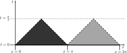
Figure 3: Schematic diagram for the solution considered here.

For the following discussion it will be convenient to reverse the time orientation, i.e. to think of the surface $t=0$ as the future boundary of the spacetime $t>0$. Due to the particular structure of the Gowdy metric Eq. (10), the light rays in the $t,x$-direction travel along $45^{\circ}$ straight lines. The left–hand dark region in Fig. 3 is hence that part of the spacetime from which no observer nor light ray can escape; all future directed causal curves in there will hit the gravitational singularity. Hence this region shares many properties with a black hole in the asymptotically flat case, and we will call this the “black hole-like region”. On the other hand, the light shaded region on the right is that part of the spacetime in which all observers and light rays will eventually cross the Cauchy horizon. Since the Cauchy horizon is a perfectly smooth surface and the gravitational field is finite there, all observers will be able to continue beyond it. Indeed, for the special choice of data above the whole light shaded region is (locally) a part of Minkowski space, i.e. there is no gravitational field at all. Note, however, that the Cauchy horizon is generated by closed null curves and hence causality breaks down. Nevertheless, we call this region the “Minkowski region”. So, the singular initial value problem allows us to construct solutions with quite peculiar properties. We expect that the part of the spacetime limited by the black hole-like and Minkowski regions to be of particular interest.

We discuss now our numerical results of this spacetime. We have demonstrated convergence of our numerical scheme in beyer10:Fuchsian12 already. In the following, we present one approximate solution which was computed with initial time at $\tau=-10$, i.e. $t\approx 5\cdot 10^{-5}$, with spatial resolution $\Delta x=10^{-3}$ and time resolution $\Delta\tau=0.0025$. In Fig. 4 we show a contour plot of the Kretschmann scalar $K$ of the spacetime, that is, the squared norm of the Riemann curvature:

$$K:=R_{\mu\nu\rho\sigma}R^{\mu\nu\rho\sigma}.$$

This is a non-trivial curvature invariant which can be considered as a measure of the gravitational strength. As expected, $K$ becomes very large close to $t=0$ inside the black hole-like region; indeed the numerical values reach $10^{15}$ very close to $t=0$. The curvature is zero insight the Minkowski region with a maximal numerical error $10^{-2}$ close to the upper tip. We consider this accuracy as sufficient for the discussion here; it would, however, be straightforward to increase the numerical accuracy even further by choosing a higher resolution or a smaller initial time of the approximate solution. Note that the fact that the curves in Fig. 4 and the following plots are slightly fuzzy is not caused by a lack of numerical accuracy of our code, but rather by the algorithm used by gnuplot to find contour lines. The plot reveals the extremely interesting dynamics here. For example note that there is an almost, but apparently not exactly flat region in the upper left corner of the figure, while there is a region in the upper right corner where the gravitational field seems to be concentrated before it collapses to the future inside the black hole-like region.

Figure 4: Contour plot of the absolute value of the Kretschmann scalar.

Motivated by our schematic understanding of the spacetime, we consider the following simple “experiment” now. Since the gravitational field collapses inside the black hole-like region and hence becomes increasingly strong there on the one hand, and since the field vanishes in the Minkowski region on the other hand, we expect that freely falling observers traveling towards $t=0$ from $t>0$ are attracted to the left-hand $x$-direction. It can be expected that these observers can only evade the black hole-like region if they are boosted sufficiently strongly to the right (but not too strongly due to periodicity in $x$). The borderline case when the observers hit the intermediate point, given by $t=0$ and $x=\pi$, and therefore “just miss” the singularity is hence particularly interesting.

Our singular initial value problem for orthogonal geodesics above allows us to compute all causal orthogonal geodesics that end in this point. The numerical result is shown in Fig. 5.

Figure 5: Causal geodesics from the intermediate point.

There we plot several orthogonal geodesics of this kind and we zoom into the region around the intermediate point. (The curve labeled by “a=0.000” will be explained shortly.) These numerical results have been obtained by solving the singular initial value problem for the orthogonal geodesic equation numerically on the numerically generated background spacetime. For this we use second-order interpolation in order to approximate the spacetime between the numerical grid points. For larger times $t$, the geodesics behave as expected; in particular they are boosted to the right in order to evade the singularity and are attracted towards the left. For times sufficiently close to $t=0$, however, the geodesics show an unexpected behavior; it seems that they are pushed away from the black hole region.

Let us describe this phenomenon in more detail and relate it to certain components of the Riemann tensor, see Fig. 6. There we show a contour plot of the $x$-component of the vector field

$$a^{\mu}:={R^{\mu}}_{ttx},$$

defined from the Riemann curvature tensor. This quantity is the relative acceleration vector of two neighboring geodesics which both start in the $t$-direction and which are separated only in the $x$-direction; see WaldBook . Its leading-order behavior for Gowdy spacetimes turns out to be

$$a^{x}=(1-k^{2})t^{-2}+\ldots$$

This is compatible with the first plot in Fig. 2 and hence is the general behavior close to any Gowdy singularity with $k<1$. It is, in particular, positive insight most of the black hole-like region in our case. In physical terms this means that such causal geodesics, which are directed away from the singularity, accelerate away from each other. Close to the intermediate point in Fig. 6, however, we see that $a^{x}$ becomes negative. Here, such causal geodesics are rather accelerated towards each other when going away from the singular region. This is a phenomenon where the effective leading-order descriptions fails; in fact, the expansion of the Riemann curvature at the intermediate point is trivial since all terms of arbitrary order vanish. However, the first of the two approximation schemes, which underlies the numerical computations, is able to unveil this reliably. We see that the region where $a^{x}$ is negative coincides exactly with that part of the spacetimes where the geodesics in Fig. 5 show the previously described surprising behavior. This is certainly a consequence of the particular choice of asymptotic data, which “concatenate” a region with very strong gravitational fields to a region with vanishing gravitational fields, that the resulting gravitational fields have this surprising property.

Figure 6: Contour plot of $a^{x}$ as defined in the text.

V Concluding remarks

In this paper we have discussed a variety of ideas relevant to the Fuchsian method and the singular initial value problem for general second–order hyperbolic Fuchsian equations and we have presented a perspective from the physics standpoint. Our method allows us, on one hand, to check under which specific conditions a given leading–order description of the dynamics of evolution equations is consistent and, on the other hand, yields two kinds of approximation schemes which allow us to go beyond this effective description and, therefore, to approximate actual solutions with in principle arbitrary accuracy. Hence, we construct solutions with prescribed singular behavior; one of the methods yields expansions of arbitrary order and hence is useful for qualitative studies; the other method approximates the actual solution by a sequence of solutions to the (standard) initial value problem and, hence, is particularly useful for numerical implementation. We stress that it is in general a challenging problem to find the correct leading–order term for the singular initial value problem associated with any given evolution equation. We have demonstrated that the proposed canonical two–term expansion yields the correct leading–order behavior in our applications, at least after some additional considerations.

We have applied this method to Gowdy spacetimes. It was discovered earlier that Gowdy solutions to Einstein’s vacuum equations can be constructed by means of the above method. In the present paper, we have in particular investigated the asymptotic dynamics of freely falling observers in such a spacetime. We confirm, as previously expected, that inhomogeneities do not effect the leading–order behavior of the geodesics; it is solely at a higher order that inhomogeneities play a significant role. In turns out that geodesics that are orthogonal to the symmetry orbits all have a limit point on the $t=0$–surface. The same conclusions also hold for non–orthogonal geodesics if $|k|<1$. If $k=\pm 1$, however, the geodesics do not in general have a limit point, but can rather “swirl” towards the singularity.

Let us mention here that, of course, it is not trivial to define geometrically what we mean by a “limit point on a curvature singularity”. Statements like “two geodesics approach the same point on the singularity” are in general rather coordinate dependent as well. For example, let us consider a family of timelike orthogonal geodesics on a Gowdy spacetime close to $t=0$ where $k$ is smaller than one which emanate from the same spatial point $x_{*}$ at $t=0$ in the sense before; the singular initial value problem above indeed allows us to construct such geodesics. Then, locally for $t>0$, we can introduce Gaussian coordinates where those geodesics represent the timelines, and therefore, with respect to these new coordinates, each of these geodesics has a different limit point on the singularity. However, such a family $\mathsf{F}_{1}$ of geodesics is indeed geometrically distinct from any family $\mathsf{F}_{2}$ where the orthogonal geodesics approach different spatial points at $t=0$ with respect to the original coordinates above. Let us consider the particle horizon in the sense of hawking at any time $t_{*}>0$ of an observer traveling away from the singularity at $t=0$ along one of the orthogonal timelike geodesics of $\mathsf{F}_{1}$. Then it follows that all the other geodesics of $\mathsf{F}_{1}$ intersect the past light-code of the observer at $t_{*}$ and are therefore never completely beyond the observer’s particle horizon, irrespective of how small $t_{*}$ is. The same situation leads to a different conclusion for the family $\mathsf{F}_{2}$; there is always a critical time $\tau_{*}$ such that any other given geodesic in $\mathsf{F}_{2}$ does not intersect the past light-cone of the observer for all $t_{*}<\tau_{*}$. Hence, two future directed observers in the case of $\mathsf{F}_{2}$ cannot communicate with each other if they are too close to the singularity. But they always can in the case of $\mathsf{F}_{1}$.

This also has consequences for the quest for a rigorous formulation of the BKL conjecture. As discussed in Rendall05 , one imagines to introduce Gaussian coordinates locally close to the singularity. The claim is that the field equations effectively decouple along each coordinate timeline and each timeline evolves as an independent Mixmaster-like universe asymptotically. Now our discussion for the Gowdy spacetimes shows that in fact, each Gaussian coordinate timeline with respect to the family $\mathsf{F}_{1}$ approaches the same, in this case, Kasner universe asymptotically. The claim of the BKL conjecture therefore only holds with respect to the family $\mathsf{F}_{2}$. Whether or not, it is possible to distinguish these two types of geodesic congruences a-priori, say, on the level of the initial data for the initial value problem, is not clear in general for a system of equations as complicated as Einstein’s field equations.

Finally, we have studied a particular Gowdy solution numerically, that is, a solution with a black hole–like region next to a Minkowski–like region exhibiting a Cauchy horizon. Of particular interest was the region where these two regions come together and interact. This led us to unexpected properties for the behavior of those causal geodesics which go into the intermediate point. It would be interesting to check whether similar phenomena are present for different types of asymptotic data. In short, we expect that the proposed theory and its generalizations (e.g. beyer:T2symm ) will be useful for various problems arising in physics and, especially, general relativity. Applying the theory to more general classes of spacetimes is work in progress.

VI Acknowledgments

Part of this paper was written in July 2011 at the Erwin Schrödinger Institute, Vienna, during the Program “Dynamics of General Relativity” organized by L. Andersson, R. Beig, M. Heinzle, and S. Husa. This paper was completed during a visit of the second author at the University of Otago in August 2011 with the financial support of the “Divisional assistance grant” of the first author (FB). The second author (PLF) was also supported by the Agence Nationale de la Recherche (ANR) via the grant 06-2–134423 “Mathematical Methods in General Relativity” and the grant “Mathematical General Relativity. Analysis and geometry of spacetimes with low regularity”.

References

- (1) F. Beyer and P.G. LeFloch, Class. Quantum Grav. 27, 245012 (2010),
- (2) F. Beyer and P.G. LeFloch, (2010), unpublished, arXiv:1004.4885 [gr-qc]
- (3) F. Beyer and P.G. LeFloch, (2010), unpublished, arXiv:1006.2525 [gr-qc]
- (4) S. Kichenassamy and A.D. Rendall, Class. Quantum Grav. 15, 1339 (1998)
- (5) A.D. Rendall, Class. Quantum Grav. 17, 3305 (2000),
- (6) J. Isenberg and S. Kichenassamy, J. Math. Phys. 40, 340 (1999)
- (7) Y. Choquet-Bruhat and J. Isenberg, J. Geom. Phys. 56, 1199 (2006),
- (8) S. Kichenassamy, Fuchsian reduction. Applications to geometry, cosmology and mathematical physics, Progress in Nonlinear Differential Equations, Vol. 71 (Springer Verlag, 2007)
- (9) Y. Choquet–Bruhat in WASCOM 2007 — 14th Conference on waves and stability in continuous media (World Sci. Publ., Hackensack, NJ, 2008), pp. 153–161
- (10) P. Amorim, C. Bernardi, and P.G. LeFloch, Class. Quantum Grav. 26, 1 (2009)
- (11) E. Ames, F. Beyer, J. Isenberg, and P.G. LeFloch, “Quasi-linear hyperbolic Fuchsian systems. Application to symmetric vacuum spacetimes”, in preparation
- (12) D. Eardley, E. Liang, and R. Sachs, J. Math. Phys. 13, 99 (1972)
- (13) J. Isenberg and V. Moncrief, Ann. Phys. 199, 84 (1990)
- (14) R. Gowdy, Ann. Phys. 83, 203 (1974)
- (15) B. Berger and V. Moncrief, Phys. Rev. D 48, 4676 (1993),
- (16) B. Berger and D. Garfinkle, Phys. Rev. D 57, 4767 (1998)
- (17) A.D. Rendall and M. Weaver, Class. Quantum Grav. 18, 2959–75 (2001)
- (18) C. Uggla, Phys. Rev. D 68, 103502 (2003)
- (19) L. Andersson, H. Van Elst, and C. Uggla, Class. Quantum Grav. 21, S29–57 (2004)
- (20) W.C. Lim, The dynamics of inhomogeneous cosmologies, Ph.D. Thesis, University of Waterloo, Canada, arXiv:gr-qc/0410126 (2004)
- (21) L. Andersson, H. Van Elst, W.C. Lim, and C. Uggla, Phys. Rev. Lett. 94, 051101 (2005)
- (22) W.C. Lim, Class. Quantum Grav. 25, 045014 (2008)
- (23) H. Friedrich, Commun. Math. Phys. 100, 525 (1985)
- (24) M. Alcubierre, Introduction to numerical relativity (Oxford Science Publications, 2008)
- (25) Y. Choquet-Bruhat, Acta Math. 88, 141 (Dec. 1952)
- (26) E. Lifshitz and I. Khalatnikov, Adv. Phys. 12, 185 (1963)
- (27) V. Belinskii, I. Khalatnikov, and E. Lifshitz, Adv. Phys. 19, 525 (1970)
- (28) V. Belinskii, I. Khalatnikov, and E. Lifshitz, Adv. Phys. 31, 639 (1982)
- (29) A.D. Rendall, Living Reviews in Relativity 8 (2005), lrr-2005-6
- (30) L. Andersson and A.D. Rendall. Commun. Math. Phys. 218:479–511 (2001).
- (31) T. Damour, M. Henneaux, A.D. Rendall, and M. Weaver. Annales Henri Poincare 3, 1049 (2002).
- (32) J.M. Heinzle and P. Sandin (2011), preprint, arXiv:1105.1643 [gr-qc].
- (33) B. Gustafsson, H. Kreiss, and J. Oliger, Time dependent problems and difference methods (Wiley Interscience Publication, 1995)
- (34) R.V. LeVeque, Finite difference methods for ordinary and partial differential equations. Steady-state and time-dependent problems (Soc. Indust. Applied Math. (SIAM), 2007)
- (35) H. Kreiss, N. Petersson, and Y. Jacob, SIAM J. Numer. Anal. 40, 1940 (2002)
- (36) L. Andersson, H. van Elst, and C. Uggla, Class. Quantum Grav. 21, S29 (2004),
- (37) J. Wainwright and G. Ellis, Dynamical Systems in Cosmology (Cambridge Univ. Press, 1997)
- (38) Y. Choquet-Bruhat and R. Geroch, Commun. Math. Phys. 14, 329 (1969)
- (39) A.H. Taub, Ann. of Math. 53, 472 ( 1951)
- (40) E. Newman, L. Tamburino, and T. Unti, J. Math. Phys. 4, 915 (1963)
- (41) P.T. Chruściel, On uniqueness in the large of solutions of Einstein’s equations (strong cosmic censorship), Proc. Centre for Mathematics and its Applications, Vol. 27 (Australian National Univ. Press, Canberra, Australia, 1991)
- (42) V. Moncrief and D. Eardley, Gen. Relativ. Gravit. 13, 887 (1981)
- (43) R. Penrose, Riv. Nuovo Cim. 1, 252 (1969)
- (44) F. Beyer and J. Hennig, (2011), preprint, arXiv:1106.2377 [gr-qc]
- (45) R. Wald, General relativity (Univ. of Chicago Press, 1984)
- (46) S.W. Hawking and G.F.R. Ellis The large scale structure of space-time (Cambridge University Press, 1973)