Evolution of the Most Massive Galaxies to $z$=0.6: I. A New Method for Physical Parameter Estimation

Abstract

We use principal component analysis (PCA) to estimate stellar masses, mean stellar ages, star formation histories (SFHs), dust extinctions and stellar velocity dispersions for a set of $\sim 290,000$ galaxies with stellar masses greater than $10^{11}M_{\odot}$ and redshifts in the range $0.4<z<0.7$ from the Baryon Oscillation Spectroscopic Survey (BOSS). We find that the fraction of galaxies with active star formation first declines with increasing stellar mass, but then flattens above a stellar mass of $10^{11.5}M_{\odot}$ at $z\sim 0.6$. This is in striking contrast to $z\sim 0.1$, where the fraction of galaxies with active star formation declines monotonically with stellar mass. At stellar masses of $10^{12}M_{\odot}$, therefore, the evolution in the fraction of star-forming galaxies from $z\sim 0.6$ to the present-day reaches a factor of $\sim 10$. When we stack the spectra of the most massive, star-forming galaxies at $z\sim 0.6$, we find that half of their [O iii] emission is produced by AGNs. The black holes in these galaxies are accreting on average at $\sim$ 0.01 the Eddington rate. To obtain these results, we use the stellar population synthesis models of Bruzual & Charlot (2003) to generate a library of model spectra with a broad range of SFHs, metallicities, dust extinctions and stellar velocity dispersions. The PCA is run on this library to identify its principal components over the rest-frame wavelength range $3700-5500$Å. We demonstrate that linear combinations of these components can recover information equivalent to traditional spectral indices such as the 4000Å break strength and H$\delta_{A}$, with greatly improved signal-to-noise ratio. In addition, the method is able to recover physical parameters such as stellar mass-to-light ratio, mean stellar age, velocity dispersion and dust extinction from the relatively low S/N BOSS spectra. We examine in detail the sensitivity of our stellar mass estimates to the input parameters in our model library, showing that almost all changes result in systematic differences in log $M_{*}$ of 0.1 dex or less. The biggest differences are obtained when using different population synthesis models – stellar masses derived using Maraston et al. (2011) models are systematically smaller by up to 0.12 dex at young ages.

1 Introduction

The mass of a galaxy is perhaps its most fundamental physical property. Many galaxy properties, such as metallicity (Tremonti et al., 2004) and recent star formation history (Salim et al., 2005; Juneau et al., 2005; Heavens et al., 2004; Kauffmann et al., 2003a), exhibit tight correlations with stellar mass. Others, such as the $\alpha-$enhancement (Thomas et al., 2004; Thomas et al., 2005; Gallazzi et al., 2006) correlate best with stellar velocity dispersion, which is a measure of the mass contained in the bulge-dominated region of the galaxy. The baryonic mass of a galaxy is correlated with the mass of the dark matter halo in which most of its stars formed (Kauffmann et al., 1997; Benson et al., 2000; Kauffmann et al., 1999; Pearce et al., 2001; Wang et al., 2006). Finally, studies of how the scaling between galaxy mass and other physical properties evolve with redshift place important constraints on the mass assembly histories of galaxies, as well as on the processes that regulate star formation and feedback in these systems (Chen et al., 2010; Wang et al., 2007).

Galaxy masses are traditionally estimated in two ways: (i) from the motions of stars and/or gas. This method measures the total mass contained interior to the radius where one measures these motions, and will include not only the the directly observed material, but also the dark matter present in the galaxy; (ii) from estimates of stellar mass-to-light ($M_{*}/L$) ratio based on fits of multi-band photometry to a grid of composite stellar population models. In the last decade, the efficiency with which multi-band photometry has been collected from ground- and space-based observatories has greatly increased, enabling stellar mass-to-light ratios to be estimated for large samples of galaxies. If spectra are available, the information carried by stellar absorption lines enables the recent star formation history of a galaxy to be more accurately determined (Kauffmann et al., 2003a; Gallazzi & Bell, 2009; Panter et al., 2004). Constraints on $M_{*}/L$ are also improved with spectroscopic information, but in practice the stellar masses estimated from multi-band photometry and spectral indices for low-redshift galaxies with luminosities $\sim L_{*}$ are consistent with less than $\sim$0.1 dex scatter (e.g., Bell et al., 2003; Drory et al., 2004; Salim et al., 2005; Borch et al., 2006). The stellar masses so obtained correlate strongly with dynamically-measured masses (e.g., Bell & de Jong, 2001; van der Wel et al., 2005; Cappellari et al., 2006).

The agreement between different methods for estimating stellar mass has led to a certain amount of complacency in the community (see Conroy et al. 2009 for a review). It is important to be aware of the following: (1)Uncertainties in the inputs to the stellar population synthesis codes used to generate the model galaxy grids are a source of systematic error in stellar mass estimation. Maraston (2005) has reported that thermally pulsing asymptotic giant branch (TP-AGB) stars contribute significantly to the near-infrared light of galaxies. Because the physics driving the pulsations is poorly understood, this phase of stellar evolution may not be very well represented in many current models. (2) At high redshifts ($z\sim 1$), one often lacks access to rest-frame near-infrared data, so star formation histories must be estimated using the shape of the spectral energy distribution (SED) in the UV/optical. This limitation can lead to systematic offsets between the stellar masses derived for galaxy samples with different redshifts, even if the true SEDs are the same (Kannappan & Gawiser, 2007). (3) If the model galaxies do not provide a correct representation of the star formation histories of the galaxies in the sample or of the transmission of the starlight to the observer, this will also lead to errors; for example, dusty galaxies and galaxies that have experienced recent starbursts have poorly-measured masses if the model library includes only galaxies with smooth star formation histories and no dust. (4) Robust stellar masses cannot be estimated if the S/N of the data is poor. This last point is perhaps an obvious one, but it is important to remember that quoted errors on stellar mass estimates are as important as the estimates themselves.

In this paper, we present a method based on a principal component analysis (PCA; Madgwick et al., 2003a; Madgwick et al., 2003b; Lu et al., 2006). to estimate galaxy physical parameters from rest-frame optical galaxy spectra using stellar population synthesis models. These parameters include stellar masses, metallicities, dust extinction, velocity dispersions, and estimates of the recent star formation histories of galaxies such as luminosity-weighted ages and the recent fraction of the stellar mass formed in bursts. Unlike much previous work, which relied on narrow-band indices defined in the vicinity of a limited set of stellar absorption lines to estimate these parameters, our method employs all the information contained in the rest-frame wavelength range of the spectrum between 3700 and 5500Å. Because our method makes use of the full spectrum, it can be applied to lower S/N data. In addition, the chosen wavelength range is accessible out to $z\sim 0.8$, even in optical spectra; this means the analysis can be applied to both low- and high-redshift galaxy samples in a consistent manner.

We apply our method to a set of spectra from the Sloan Digital Sky Survey Data Release 7 (DR7; Abazajian et al., 2009), as well as a new sample of 290,000 spectra of luminous galaxies from the Baryonic Oscillation Spectroscopic Survey (BOSS; Eisenstein et al., 2011; Schlegel et al., 2009). We present spectrum-based stellar mass estimates for these galaxies, as well as their recent star formation histories, and use this information to assess how the recent star formation histories of the most massive galaxies in the Universe have evolved from $z\sim 0.55$ to the present day.

Our paper is arranged as follows. In §2, we introduce the two data sets. Our methodology for estimating stellar mass and recent SFH is developed in §3. The improvements of this new method are discussed in §4. We compare our stellar masses with those from multi-band photometry in §5. We also discuss systematic effects in our estimates of stellar mass. Our results on the evolution of massive galaxies are presented in §6. We use the cosmological parameters $H_{0}=70~{}{\rm km~{}s^{-1}~{}Mpc^{-1}}$, $\Omega_{\rm M}=0.3$ and $\Omega_{\Lambda}=0.7$ throughout this paper.

2 The SDSS Data

2.1 SDSS DR7

The Sloan Digital Sky Survey (SDSS; York et al., 2000) obtained photometry of nearly a quarter of the sky and spectra of about one million objects. A drift-scanning mosaic CCD camera (Gunn et al., 1998) mounted on the SDSS 2.5m telescope at Apache Point Observatory (Gunn et al., 2006) imaged the sky in the $u,g,r,i,z$ bands (Fukugita et al., 1996). The imaging data are astrometrically (Pier et al., 2003) and photometrically (Hogg et al., 2001; Padmanabhan et al., 2008) calibrated and used to select stars, galaxies, and quasars for follow-up fiber spectroscopy.

The seventh data release (Abazajian et al., 2009) of the SDSS includes $\sim$930,000 galaxy spectra. The spectra have a wavelength coverage of $3800-9200$Å and are taken through $3^{\prime\prime}$ diameter fibers. The instrumental resolution is $R\sim 2000$ and the dispersion is $\Delta{\rm log}\lambda=10^{-4}$, where $\lambda$ is the wavelength in Angstroms. The median S/N per pixel of the spectra ranges from 4 to 30, with a median of 14. In this paper, we make use of the spectra of galaxies from the “Main Sample” (Strauss et al., 2002), which have Petrosian magnitudes in the range $14.5<r<17.6$ after correction for foreground galactic extinction using the reddening maps of Schlegel et al. (1998). The redshift range spanned by these galaxies is 0.01 to 0.30 (see Figure 1).

Stellar masses and star formation rate for the Main Sample have been publicly available since 2008 in the MPA/JHU catalog. The stellar masses are estimated from broad-band $u,g,r,i,z$ photometry (“model” fluxes are used, see Stoughton et al. (2002) for definitions of the magnitudes). The total fluxes are corrected for emission line contribution by assuming that the relative contribution of emission lines to the broad-band magnitudes is the same inside the fiber as outside. A large grid of model star formation histories is generated following the methodology described in Kauffmann et al. (2003a), and comparison of the observed colors with predictions from these models allows one to derive maximum likelihood estimates of the $z$-band stellar mass-to-light ratios ($M_{*}/L_{z}$) of the galaxies. Stellar masses are computed by multiplying $M_{*}/L_{z}$ by the $z$-band “model” luminosity $L_{z}$. Masses derived from the 5-band photometry are consistent with previous stellar masses derived using spectral features (D4000 & H$\delta_{A}$ in the case of Kauffman et al. 2003a and a total of five indices in the case of Gallazzi et al. 2005) with an r.m.s scatter of 0.1 dex in log $M_{*}$. The SFRs are derived from nebular emission lines (Brinchmann et al., 2004).

The large wavelength coverage and high S/N of the DR7 spectra, and the fact that robust stellar mass estimates are publicly available, means that the DR7 main sample (hereafter we refer this sample as the DR7 sample for convenience) is very well-suited for developing and testing our new method of physical parameter estimation (see §5).

2.2 Baryon Oscillation Spectroscopic Survey

The SDSS-III project has completed an additional 3000 ${\rm deg}^{2}$ of imaging in the southern Galactic cap in a manner identical to the original SDSS imaging (Aihara et al., 2011). BOSS is obtaining spectra of a selected subset of 1.5 million luminous galaxies to $z\sim 0.7$. (N. Padmanabhan et al. 2011, in preparation). The spectrographs have been significantly upgraded from those used by SDSS-I/II, with improved CCDs with better red response, high throughput gratings, and an increased number of fibers (1000 instead of 640). The new fibers are $2^{\prime\prime}$ in diameter and the spectra cover the wavelength range 3600$-$10,000Å, at a resolution of about 2000. The BOSS galaxy spectra have median S/N per pixel ($\Delta{\rm log}\lambda=10^{-4}$) of $\sim$2.5.

The details of how targets are selected from the SDSS photometry will be described in detail in Padmanabhan et al. (in preparation). The sample we analyze here is the “CMASS” sample (so-named, because it is very approximately stellar-mass limited). The sample is defined using the following cuts:

$$\begin{array}[]{c}d_{\perp}>0.55\quad{\rm and}\quad 17.5<i<19.9\quad{\rm and}\quad i_{\rm fiber2}<21.5\\ i<19.86+1.6\,(d_{\perp}-0.8)\quad{\rm and}\quad r-i<2\end{array}$$ (1)

where $d_{\perp}$ is a “rotated” combination of colors defined as $d_{\perp}=(r-i)-(g-r)/8$. $i_{\rm fiber2}$ is the magnitude of the galaxy measured within a $2^{\prime\prime}$ diameter aperture; this is the amount of light that enters the fiber. We note that all color cuts are defined using “model” magnitudes, whereas magnitude limits are given in terms of “cmodel” magnitudes. Two additional cuts are introduced to reduce contamination by stars; $z_{\rm psf}-z_{\rm model}\geq 9.125-0.46\,z_{\rm model}$ and $i_{\rm psf}-i_{\rm model}>0.2+0.2\times(20.0-i_{\rm model})$ (“psf” refers to the $psfMag$ quantity in the SDSS database). Redshifts are successfully determined for 95.3% of CMASS galaxies with no apparent dependence on galaxy type.

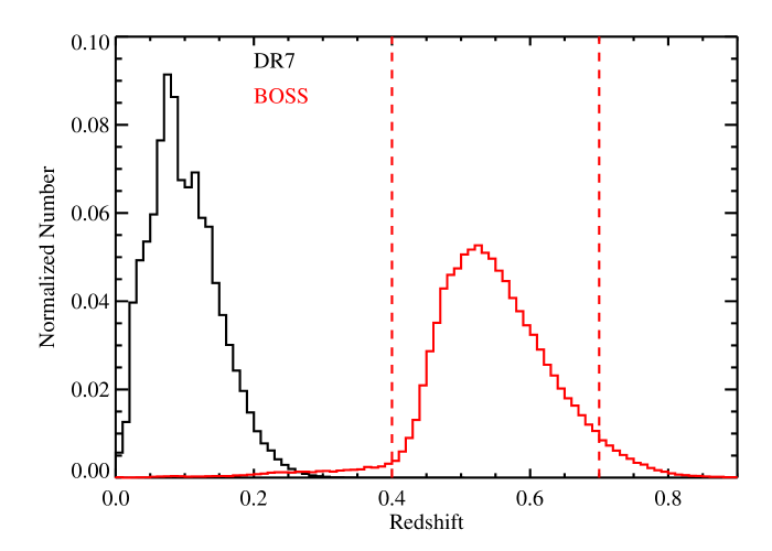
Figure 1: Black: the redshift distribution of the DR7 sample; red: the redshift distribution of the“CMASS” sample of BOSS high-$z$ luminous galaxies. The two vertical dashed lines indicate the redshift limits of the “CMASS” sample used in our analysis.

These cuts are designed to select massive galaxies with $z>0.45$. The constraint that $d_{\perp}>0.55$ identifies galaxies that lie at high enough redshift so that the 4000 Å break has shifted beyond the observer frame $r$-band, leading to red $r-i$ colors. The cut on the $i$-band magnitude of the galaxy is designed to produce a sample that is roughly complete down to a limiting stellar mass of ${\rm log}M_{*}\sim 11.2$ (we will come back to this point later). The analysis presented in this paper includes the $\sim 290,000$ CMASS spectra obtained prior to July 2011 which will be made publicly available in SDSS Data Release 9. We restrict our analysis to galaxies in the redshift range $0.4<z<0.7$ (see Figure 1).

3 The method

Because the CMASS galaxies are faint, the errors on the broad-band colors are large; this is especially true of colors that include the $u$-band. The median magnitude errors are 0.62, 0.16, 0.06, 0.04, 0.09 for $u,g,r,i,z$-band measurements, respectively. In this section, we describe a new method for estimating galaxy properties, including stellar masses and recent SFHs, using the SDSS spectra rather than photometry. As we will show, this method can be applied successfully to low S/N data, such as that from the BOSS survey.

The main concept underlying our approach is the fact that a galaxy spectrum can be described as a number of orthogonal principal components (PCs). When one applies a PCA decomposition to model galaxy spectra, one finds that the PCs can be related to the physical properties of galaxies, such as their stellar mass-to-light ratios, their recent SFHs, the average age of their stellar populations, and their velocity dispersions. By decomposing each observed spectrum into the same set of PCs, and by comparing the amplitudes of the components with those calculated for the model galaxies, we obtain the likelihood distribution of a given parameter $P$ in the space of the values of $P$ allowed by the models. In this work, we calculate likelihood distributions by comparing the amplitudes of the first seven PCs (§3.4.1 clarifies this choice) to those calculated for the galaxies in the model library. In the following sections, we provide a step-by-step description of our method.

3.1 The spectral range used in the analysis

We follow two criteria to select the rest-frame spectral range: (1) it should be as wide as possible so as to make optimum use of all the information carried in the spectrum; (2) to minimize systematic effects, the same spectral range should be used in the analysis of both the low redshift and the high redshift galaxies. Considering the redshift and wavelength coverage of DR7 ($0.005<z<0.3$, $3800<\lambda<9200$Å) and of BOSS ($0.4<z<0.7$, $3600<\lambda<10,000$Å) galaxy samples, we choose rest-frame 3700Å to 5500Å for the current analysis. Spectral features located in this region, including the 4000Å break strength (D4000) and Balmer absorption lines, provide important information about the stellar populations and recent SFHs of the galaxies.

Single stellar population (SSP) models that are well-matched in spectral resolution (e.g. from Bruzual & Charlot 2003, hereafter BC03 and from Maraston & Stromback 2011, hereafter M11) are also available over this wavelength range. BC03 has a spectral resolution of 75 ${\rm km~{}s}^{-1}$, while M11 spectral resolution is 65 ${\rm km~{}s}^{-1}$, similar to the instrumental resolution, $\sim 75~{}{\rm km~{}s}^{-1}$, of the DR7 and BOSS spectra.

3.2 Model library

We generate a library containing 25,000 realizations of different SFHs using SSP models from BC03. The model library is parametrized as follows

1. SFHs. Each SFH consists of three parts: a) an underlying continuous model, b) a series of super-imposed stochastic bursts, c) a random probability for star formation to stop exponentially (i.e. truncation). In the continuous model, stars are formed from the time $t_{\rm form}$ to the present according to the following functional form: ${\rm SFR}(t)\propto{\rm exp}[-\gamma(t-t_{\rm form})]$. The formation time $t_{\rm form}$ is uniformly distributed between 13.5 and 1.5 Gyr and the star formation inverse time-scale $\gamma$ is uniformly distributed over the range 0$-$1 Gyr^-1. The main parameter that controls the bursts is the amplitude $A$, defined as the fraction of stellar mass produced during the burst relative to the total mass formed by the continuous model. $A$ is logarithmically distributed between 0.03 and 4. During the burst, stars are formed at a constant rate that is independent of $A$ for a time $t_{\rm burst}$, which is uniformly distributed between $3\times 10^{7}-3\times 10^{8}$yr. Bursts occur at all times after $t_{\rm form}$ with equal probability. The probability is set in such a way that 15% of the galaxies in the library experience a burst in the last 2 Gyr.

   The existence of a population of massive, compact “post-starburst” galaxies at high redshifts with little or no ongoing star formation (e.g., Kriek et al., 2006; Kriek et al., 2009) has triggered us to add possible truncations to the SFHs. For 30% galaxies in the library, we truncate the star formation at a random time in the past. Following the truncation event, the star formation rate evolves as ${\rm SFR}(t>t_{\rm cut})\sim{\rm SFR}(t_{\rm cut})~{}{\rm exp}[-(t-t_{\rm cut})/\tau]$, where $t_{\rm cut}$ is the truncation time and log$\tau$ is uniformly distributed in the range 7 to 9. We note that in Kauffmann et al. (2003a), the fraction of galaxies with bursts in the last 2 Gyr was set to be 50%. We have reduced this fraction to 10% (after truncations are included) because it provides a more uniform distribution in the light-weighted age of the models. The influence of the choice of the fraction of galaxies with recent bursts on our physical parameter estimation is discussed in §5.3.

2. Metallicity. The BC03 model library includes six metallicities ranging from 0.005 to 2.5$Z_{\odot}$; we interpolated the BC03 model grids in metallicity in log-space. 95% of the model galaxies in our library are distributed uniformly in metallicity from $0.2-2.5Z_{\odot}$; 5% of the model galaxies are distributed uniformly between $0.02$ and $0.2Z_{\odot}$. The reason for including these very low metallicity models is that Maraston et al. (2009) have found that the colors predicted for simple single stellar populations do not provide a good match to the observed colors of the reddest galaxies in the SDSS. Adding a small fraction (typically 3% of the total stellar mass) of old metal-poor stars allows one to achieve a significantly better match to the observations.

3. Dust extinction. Dust extinction is modelled using the two-component model described in Charlot & Fall (2000). The $V$-band optical depth has a Gaussian distribution over the range $0<\tau_{V}<6$, with a peak at 1.2 and 68% of the total probability distribution distributed over the range $0-2$. Our adopted prior distribution of $\tau_{V}$ values is motivated by the observed distribution of Balmer decrements in SDSS spectra (Brinchmann et al., 2004). The fraction of the optical depth that affects stellar populations older than $10^{7}$yr is parametrized as $\mu$, which is again modeled as a Gaussian with a peak at $\mu=0.3$ and a 68 percentile range of $0.1-1$.

4. Velocity dispersion. Each of the model spectra is convolved to a velocity that is uniformly distributed over the range of values from 50 to 400${\rm km~{}s}^{-1}$.

We adopt the universal initial mass function (IMF) given in Kroupa (2001). For each model in the library, we store the following properties:

1. the spectrum over the wavelength range ($91-160,000$Å);

2. the strengths of the D4000 and H$\delta_{A}$ indices, measured in the same way as in the SDSS spectra;

3. the $r$-band luminosity-weighted age, which is defined as $t_{r}=\int_{0}^{t}[d\tau~{}{\rm SFR}(t-\tau)~{}f_{r}(\tau)~{}\tau]/\int_{0}^{t}[d\tau~{}{\rm SFR}(t-\tau)~{}f_{r}(\tau)]$, where $f_{r}(\tau)$ is the total $r$-band flux produced by stars at age $\tau$;

4. the mass-weighted age, which is calculated as $t_{m}=\int_{0}^{t}[d\tau~{}{\rm SFR}(t-\tau)~{}\tau]/\int_{0}^{t}[d\tau~{}{\rm SFR}(t-\tau)]$;

5. the $i$-band and $z$-band stellar mass-to-light ratios, $M_{*}/L_{i}$ and $M_{*}/L_{z}$, of the model at redshifts between 0 and 0.8 in steps of $z=0.05$. Note that we account for the fraction of the initial stellar mass that is returned to the interstellar medium by evolved stars (e.g., we output the mass of living stars and remnants, not the mass formed);

6. the star formation history, including fraction of stars formed in recent bursts, time of truncation etc.;

7. the metallicity;

8. the dust parameters $\tau_{V}$ and $\mu$;

9. the stellar velocity dispersion;

The choice of priors is important in Bayesian analysis; we test the dependence of our stellar mass estimations on the input parameters of the model library in §5.2.

3.3 Identifying the significant principal components of the spectral library

Our method makes use of Principle Component Analysis (PCA) , a standard multivariate analysis technique (see Budavari et al 2009., for a recent discussion). A spectrum containing M wavelength points can be regarded as a single point in an M-dimensional space. A group of spectra form a cloud of points in this space. PCA searches for a vector (principal component) which has as high a variance as possible in the cloud of points. Each succeeding component in turn has the highest variance possible under the constraint that it be orthogonal to (i.e. uncorrelated with) the preceding components.

Before we run the PCA code on the library of models, we mask the regions around nebular emission lines in the model spectra. Our models do not include emission lines, and it is important to treat the models and the real data in exactly the same manner. We mask 500 ${\rm km~{}s}^{-1}$ around the [O ii]3726.03, [O ii]3728.82, H₈3889.05, [Ne iii]3869.06, H$\gamma$4101.73, H$\delta$4340.46, H$\beta$4861.33, [O iii]4959.91, and [O iii]5007.84Å lines. Each spectrum in the masked library is normalized to its mean flux between $3700-5500$Å.

Let us express the $i$-th normalized spectrum as $S_{i,k_{\lambda}}$, where $i$ is an integer running over the 25,000 model galaxies and $k_{\lambda}$ is an integer running over each pixel in the spectrum. We calculate the mean spectrum of the masked library and subtract this from each of the model spectra. We then run our PCA code on the “residual” spectra. Figure 2 presents the mean spectrum and the first seven PCs for our input model library.

Figure 2: From top to bottom: the mean spectrum of the model library followed by the first to the seventh eigenspectra.

As expected, the mean spectrum is typical of that of a galaxy with an intermediate age stellar population. The first PC is relatively featureless. As we will show, it provides a first-order measure of the age of the stellar population and it is strongly correlated with both 4000Å break and Balmer absorption lines strengths. The second PC is quite noisy, but as we will show in §3.4.1, it encodes information about the stellar velocity dispersion of the galaxy. The third PC contains information about velocity dispersion and metallicity. The fourth PC clearly recovers information contained in the Balmer absorption lines, even though the line centers have been masked. CaII (H+K) and Mgb absorption lines are clearly visible in the fifth PC; as we will show this component carries much information about galaxy metallicity. It is difficult to determine what information is encoded in the sixth and seventh PCs by simple visual inspection. In the next section, we present a more quantitative analysis that demonstrates that these two PCs encode information about velocity dispersion and metallicity, respectively.

3.4 Decomposing each model and observed spectrum into its PC representation

3.4.1 Projection of the model library

The $i$-th model spectrum $S_{i,k_{\lambda}}$ is projected onto the eigenspectra as follows:

$$S_{i,k_{\lambda}}=M_{k_{\lambda}}+\sum_{\alpha}C^{m}_{i,\alpha}~{}E_{\alpha,k_{\lambda}}+R_{i,k_{\lambda}},$$ (2)

where $M_{k_{\lambda}}$ is the mean spectrum of the model library. The integer $k_{\lambda}$ indexes the rest-frame wavelength bin of the spectrum. $C^{m}_{i,\alpha}$ is the amplitude of the $\alpha$-th PC $E_{\alpha,k_{\lambda}}$ (Note that $\alpha$ ranges from 1 to 7, and the superscript $m$ refers to to the fact that the models are being projected onto PC space in this section). $C^{m}_{i,\alpha}$ can be expressed as

$$C^{m}_{i,\alpha}=\sum_{k_{\lambda}}(S_{i,k_{\lambda}}-M_{k_{\lambda}})~{}E_{\alpha,k_{\lambda}}.$$ (3)

$R_{i,k_{\lambda}}$ is the residual of the $i$-th spectrum from its PC representation (it can be regarded as a measure of the theoretical “noise” in the decomposition). The covariance matrix of the theoretical “noise” can be written as

$$Cov^{\rm th}_{k_{\lambda},k_{\lambda}^{\prime}}=(1/N_{\rm mod})\sum_{i=1,N_{\rm mod}}(R_{i,k_{\lambda}}R_{i,k^{\prime}_{\lambda}})$$ (4)

where $N_{\rm mod}$ is the number of models in the library (note that this noise covariance is indexed by rest-frame wavelength).

Although the PC representation of spectra is compact and mathematically convenient, it is not a priori clear what physical information is encoded in each of the components. In some cases (see Figure 2), one can simply eyeball the eigenspectrum and make an educated guess as to its “meaning”, but in other cases very little can be gleaned from simple visual inspection.

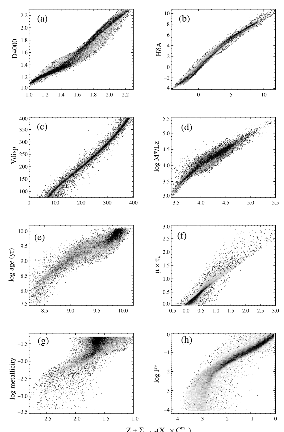
Figure 3: The correlation between 8 different model galaxy spectral properties or parameters: (a) D4000; (b) H$\delta_{A}$; (c) velocity dispersion; (d) $z$-band stellar mass-to-light ratio; (e) luminosity-weighted age; (f) dust extinction; (g) metallicity; (h) the fraction of stars formed in the last Gyr, and the linear combination of $C^{m}_{\alpha}$ that minimizes the scatter in the correlation (see text). The values of the coefficient $X_{\alpha}$ and the zero point $Z$ for each case are listed in Table 1.

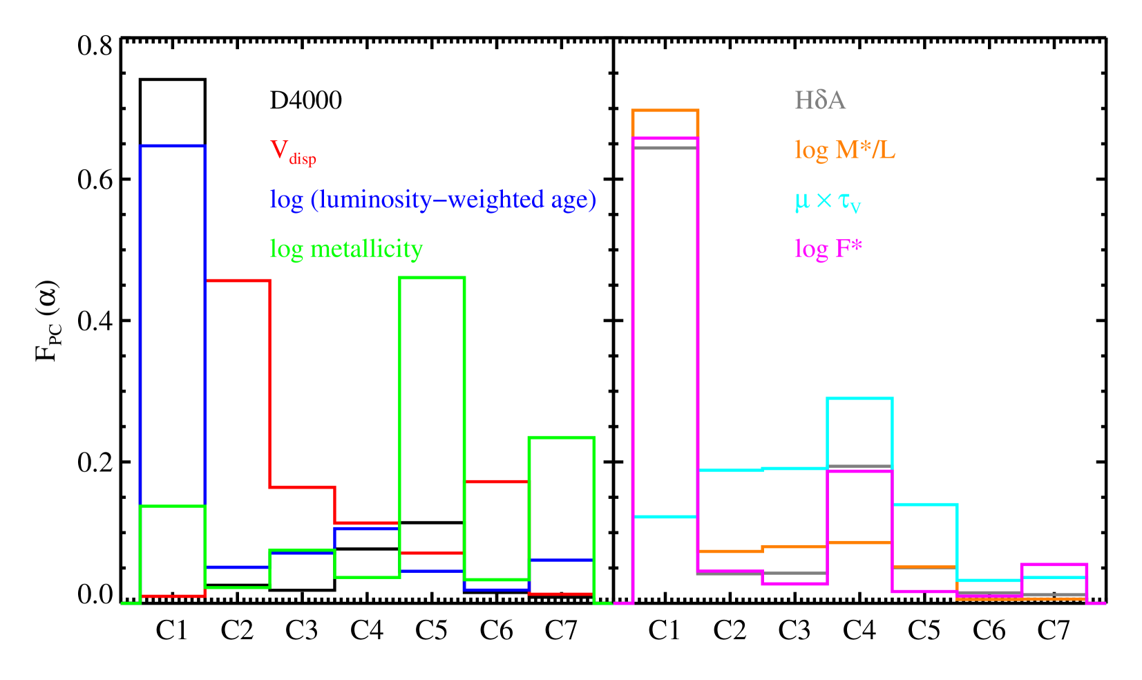
Figure 4: This figure shows the relative contribution of each PC to the same spectral properties/parameters displayed in Figure 3. They are color-coded as follows: Black $-$ D4000; red $-$ velocity dispersion; blue $-$ luminosity-weighted age; green $-$ metallicity; grey $-$ H$\delta_{A}$; orange $-$ stellar mass-to-light ratio; cyan $-$ dust extinction; magenta $-$ fraction of stars formed in the last Gyr.

In order to develop a better understanding of the information encoded in the PCs , we search for the best correlation between $Z+\sum_{\alpha}(X_{\alpha}\times C^{m}_{\alpha}$) and a variety of galaxy parameters ($P$) that we store for each model spectrum (examples of $P$ include spectral properties such as D4000, H$\delta_{A}$, and velocity dispersion ($V_{\rm disp}$), as well as model parameters such as stellar mass-to-light ratio, light-weighted age, dust extinction, metallicity, and fraction of stars formed in the last 1 Gyr ($F_{*}$)). This can be thought of as finding the linear combination of the PC amplitudes that best predicts the parameter $P$ when averaged over all the model spectra in the library. The zero point $Z$ and coefficients $X_{\alpha}$ are calculated by minimizing

$$\Delta=\sum_{i=1}^{N_{\rm mod}}\big{[}\sum_{\alpha}X_{\alpha}\times C^{m}_{i,\alpha}+Z-P_{i}\big{]}^{2}.$$ (5)

When we perform this exercise, we increase the number of PCs used in the projection one at a time, each time checking the mean correlation between $Z+\sum_{\alpha}(X_{\alpha}\times C^{m}_{\alpha}$) and $P$ as well as its scatter . We find that our results converge when $\alpha=$7; and therefore use the first seven PCs in our analysis.

Table 1: Values of $X_{\alpha}$ and $Z$ for each spectral property or physical parameter $P$

$P$	$C_{1}$	$C_{2}$	$C_{3}$	$C_{4}$	$C_{5}$	$C_{6}$	$C_{7}$	$Z$
(1)	(2)	(3)	(4)	(5)	(6)	(7)	(8)	(9)
D4000	0.049	$-$0.018	0.016	0.083	$-$0.168	0.039	0.029	1.619
H$\delta_{A}$	$-$0.517	0.369	$-$0.460	$-$2.551	0.905	$-$0.454	$-$0.497	2.808
$V_{\rm disp}$	0.267	135.517	$-$59.563	50.294	$-$42.942	$-$176.941	17.609	226.919
log $M_{*}/L_{z}$	$-$0.051	$-$0.059	$-$0.079	0.103	$-$0.084	0.015	$-$0.022	$-$4.209
log age(yr)	0.071	$-$0.061	$-$0.105	0.189	0.111	0.078	0.340	9.385
$\mu\times\tau_{V}$	0.017	0.295	0.366	$-$0.678	0.445	$-$0.176	$-$0.265	0.528
log metallicity	0.009	$-$0.017	0.070	$-$0.041	$-$0.710	$-$0.088	$-$0.821	$-$1.692
log $F_{*}$	$-$0.437	0.333	$-$0.245	$-$2.032	$-$0.248	$-$0.259	$-$1.855	$-$3.631

Figure 3 shows the correlations between $Z+\sum_{\alpha}(X_{\alpha}\times C^{m}_{\alpha}$) and a variety of different galaxy parameters $P$. We have included D4000 and H$\delta_{A}$ in this set even though they are not physical parameters, because they were used extensively in our previous work and we would like to understand how they relate to our new system of PCs. In addition, we include stellar velocity dispersion, $i$-band mass-to-light ratio, $r$-band light-weighted mean stellar age, metallicity, dust extinction and the fraction of stars formed in the last Gyr. We see that we are able to recover very accurate estimates of D4000, H$\delta_{A}$, velocity dispersion and dust content from the principal components. This is not surprising, because the 4000 Å break and the Balmer absorption lines are the strongest features present in the spectra for the wavelength range that we have chosen. Likewise, increasing extinction and velocity dispersion modify the shape of the spectrum and the width of the spectral features in a roughly linear way, so it is expected that the correlation with the appropriate combination of PC components will be very tight.

On the other hand, there are well known degeneracies between stellar age and metallicity that affect many stellar features (Oconnell, 1986). In past work, certain specific features have been identified as being key to breaking this degeneracy (e.g., Worthey, 1994; Vazdekis & Arimoto, 1999; Maraston & Thomas, 2000; Le Borgne et al., 2004), so it is interesting to see whether our PCA technique is capable of doing the same. In Figure 3, Panels (d) and (e) indicate that one is able to recover reasonably accurate estimates of stellar mass-to-light ratio and mean stellar age. Panel (h) shows that our method is able to cleanly identify galaxies in which more than $\sim$ 1% of the stellar population formed in the last Gyr. Panel (g) shows that metallicity can be recovered for values that are below solar ($\rm{log~{}metallicity}<-1.7$). We note, however, that we have not yet considered the effect of varying element abundance ratios, which significantly complicates metallicity estimation in real elliptical galaxies (Thomas et al., 2002).

In Table 1, we list the set of $X_{\alpha}$ and $Z$ values for each parameter $P$. In Figure 4, we attempt to illustrate the relative “importance” of each of the PC components in estimating different galaxy parameters. We define $F_{\rm pc}(\alpha)$ as

$$F_{\rm pc}(\alpha)=\frac{\sum_{i=1}^{N_{\rm mod}}|X_{\alpha}\times C^{m}_{i,\alpha}|}{\sum_{\alpha=1}^{7}\sum_{i=1}^{N_{\rm mod}}|X_{\alpha}\times C^{m}_{i,\alpha}|}.$$ (6)

The results are shown in Figure 4. For each parameter $P$ in Figure 3, we plot $F_{\rm pc}$ as a function of $\alpha$, where $\alpha$ is the index of the PC component. The results are largely consistent with our previous discussion of Figure 2. Information about D4000, H$\delta_{A}$, stellar mass-to-light ratio, light-weighted age and the fraction of stars formed in the last Gyr is primarily contained in PC1, with lesser contributions from PC4 and PC5. As we have discussed, PC1 provides a measure of the continuum shape, whereas PC4 is similar to the component defined in Wild et al (2007) that provides a measure of the “bursty” nature of the past star formation history. Information about velocity dispersion is encoded in PC2, PC3 and PC6. Information about metallicity is mainly contributed by PC5 and PC7. Interestingly, PC components 2 through 5 contribute almost equally in the estimation of stellar mass-to-light ratio.

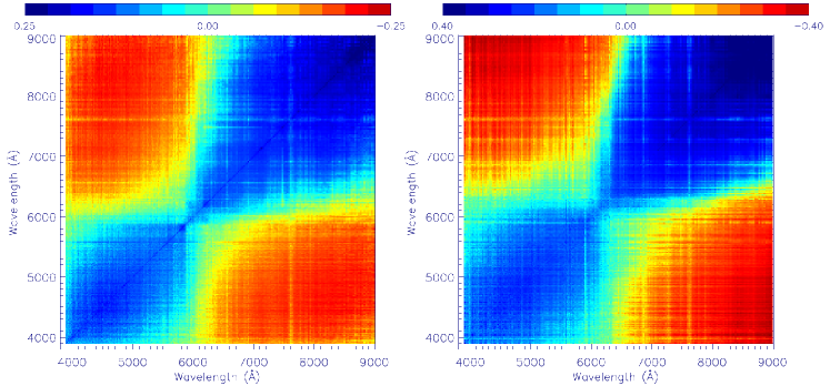
Figure 5: The rescaled mean observational error covariance matrix $Cov_{l_{\lambda},l_{\lambda}^{\prime}}$ in the wavelength interval of $4000-9000$Å derived from DR7 repeat spectra (left) and BOSS repeat spectra (right).

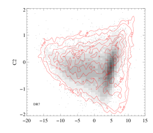
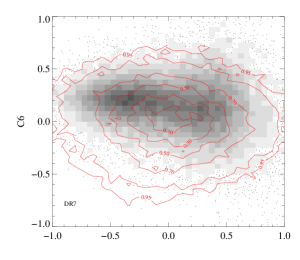
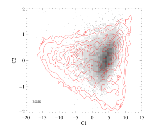
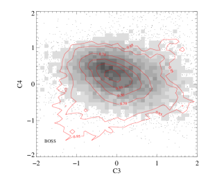
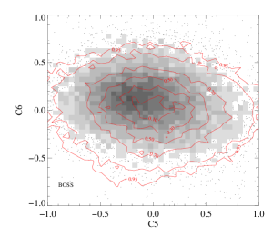
Figure 6: This figure shows $C_{1}$ vs. $C_{2}$, $C_{3}$ vs. $C_{4}$ and $C_{5}$ vs. $C_{6}$ for DR7 galaxies (top) and for BOSS galaxies (bottom). Models are shown in red contours, while data is shown in grey scales. We have convolved the model spectra with the errors appropriate for DR7 and CMASS when generating the PCA components for this plot. The outermost contour encloses 95% of the models.

3.4.2 Projection of the real data

In this section, we describe how we apply the PCA methodology to observed galaxy spectra. The steps are as follows:

1. The galaxy spectra are corrected for foreground Galactic extinction and the wavelength scale is shifted from vacuum to air to match the models.

2. The set of emission lines listed in §3.3 are masked. In addition, we found it necessary to mask $500{\rm km~{}s}^{-1}$ around H i3770.63, 3797.90, 3835.38, 3889.049, 3970.072, 4101.734, 4340.464, He i4387.93, 5047.74, He ii5015.68, [Ne iii]3967.79, [O iii]4364.21Å lines in the subset of strong emission line galaxies with EQW of H$\beta$ $<-$5 (12% of DR7, 1% of CMASS). We have checked that our results are robust to the choice of mask size.

3. The observed spectrum and its error array are normalized by dividing by the flux density averaged over the full observed wavelength range. We then apply an integer pixel offset to shift them from observed to rest-frame wavelength. We denote the normalized flux density and its error arrays as $O_{k_{\lambda}}$ and ${\rm Eps}_{k_{\lambda}}$, respectively. For “bad” pixels and night sky lines identified in the SDSS mask array, we set the pixel values in the observed normalized spectrum, $O_{k_{\lambda}}$, proportional to the value in the mean spectrum of the model library, $a\times M_{k_{\lambda}}$, where $a$ is the mean flux of $O_{k_{\lambda}}$ between rest frame $3700-5500$Å, which takes the different normalizations between models and data into account. (We choose this normalization of the data for the convenience of estimating the mean observational error covariance matrices, see Eq. 9). The corresponding pixel values in the error array are set to 10 times the mean error of all the good pixels.

4. The coefficients of the PC components of the observed spectrum are

   $$C_{\alpha}^{d}=\sum_{k_{\lambda}}(O_{k_{\lambda}}-a\times M_{k_{\lambda}})~{}E_{\alpha,k_{\lambda}}.$$ (7)

   Note that the index $k_{\lambda}$ ranges over the pixels between 3700$-$5500Å in the rest frame.

3.4.3 Error estimation for the PC coefficients $C_{\alpha}^{d}$

This section describes how we estimate the errors on $C_{\alpha}^{d}$ as calculated in equation (7). Let us write the observed spectrum over the restricted wavelength range we are modeling as

$$O_{k_{\lambda}}=a\times M_{k_{\lambda}}+\sum_{\alpha}C^{true}_{\alpha}~{}E_{\alpha,k_{\lambda}}+N^{th}_{k_{\lambda}}\times a+N^{obs}_{k_{\lambda}}$$ (8)

where the first two terms in equation (8) represent the “true” PC representation of the galaxy in the absence of errors of any sort. $N^{th}_{k_{\lambda}}$ and $N^{obs}_{k_{\lambda}}$ are independent Gaussian noise vectors representing the “theoretical” and the “observational” errors. These two noise vectors have covariance matrices $Cov^{th}_{k_{\lambda},k^{\prime}_{\lambda}}$ and $Cov^{obs}_{k_{\lambda},k^{\prime}_{\lambda}}$, respectively.

$Cov^{th}_{k_{\lambda},k^{\prime}_{\lambda}}$ is the same for each observed galaxy and is given by equation (4). The covariance matrix of the observational errors differs from one galaxy to the next. The diagonal terms are given by ${\rm Eps}^{2}_{k_{\lambda}}$, the square of the normalized error array of the particular galaxy in question. The off-diagonal terms are somewhat tricky to evaluate, because they depend on details of the instrumental response, flux calibration errors, etc.

Both the DR7 main galaxy sample and the BOSS CMASS sample include a large number of galaxies that were observed multiple times, due to overlaps between different spectroscopic fiber plug plates. These “repeat spectra” are extremely useful for assessing uncertainties in a variety of estimated quantities. We identify a sample of 48,000 “repeat galaxy spectra” for DR7 (19,000 for CMASS); these two samples are used to construct the mean observational error covariance matrices for DR7 and CMASS galaxies as

$$Cov_{l_{\lambda},l_{\lambda}^{\prime}}=\\ \frac{1}{2N_{\rm pair}}\sum_{j=1,N_{\rm pair}}(O_{j,1,l_{\lambda}}-O_{j,2,l_{\lambda}}).(O_{j,1,l_{\lambda}^{\prime}}-O_{j,2,l_{\lambda}^{\prime}})$$ (9)

where $O_{j,a,l_{\lambda}}$ is the normalized flux of the $a$-th observation ($a$ = 1 or 2) of the $j$-th pair. Bad pixels are replaced by the median of 200 neighbouring pixels. $l_{\lambda}$ ranges over all the pixels in the spectrum. Note that in contrast to the index $k_{\lambda}$ used above, $l_{\lambda}$ indexes wavelength in the observed frame, and $O_{j,a,l_{\lambda}}$ refers to the observed spectrum.

In Figure 5, we show a diagrammatic representation of the observational covariance matrices from the DR7 and BOSS repeat observations over the wavelength interval of $4000-9000$Å. We have stretched the scale in order to distinguish positive from negative values and to have a near-logarithmic scale near zero (in practice, we plot sign($Cov_{l_{\lambda},l_{\lambda}^{\prime}}$)$|Cov_{l_{\lambda},l_{\lambda}^{\prime}}|^{0.3}$). The absolute values of the elements on the BOSS mean observational error covariance matrix are much larger than that for DR7, reflecting the fact that the BOSS data are at lower S/N. The strong shift in sign at 6000 Å reflects the change between the blue and the red channels of the SDSS spectrograph. When using the matrices below (see equation 11), the off-diagonal terms of $Cov^{obs}_{k_{\lambda},k^{\prime}_{\lambda}}$ are set to be the values of $Cov_{l_{\lambda},l_{\lambda}^{\prime}}$ at the corresponding observer-frame wavelength.

The difference between “true” and estimated PC coefficients is

$${\rm d}C_{\alpha}=C^{true}_{\alpha}-C^{d}_{\alpha}=\sum_{k_{\lambda}}E_{\alpha,k_{\lambda}}~{}(N^{th}_{k_{\lambda}}\times a+N^{obs}_{k_{\lambda}})$$ (10)

The covariance matrix of this difference (i.e the covariance in the errors on the different PC coefficients) is then given by

$$\begin{array}[]{lcl}Cov^{\rm pc}_{\alpha,\alpha^{\prime}}=<{\rm d}C_{\alpha}~{}{\rm d}C_{\alpha^{\prime}}>=\\ \sum_{k_{\lambda},k^{\prime}_{\lambda}}[E_{\alpha,k_{\lambda}}\times(Cov^{\rm th}_{k_{\lambda},k^{\prime}_{\lambda}}\times a^{2}+Cov^{\rm obs}_{k_{\lambda},k^{\prime}_{\lambda}})\times E_{\alpha^{\prime},k^{\prime}_{\lambda}}]\end{array}$$ (13)

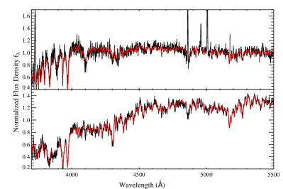
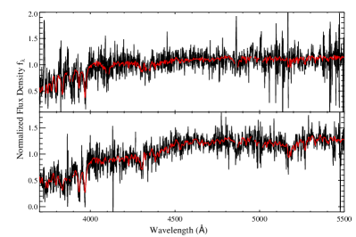
Figure 7: Left panel: Example DR7 spectra (black) and the corresponding PCA fits (red) for a late-type galaxy (top) and an early-type galaxy (bottom). The spectrum is plotted over the wavelength interval $3700-5500$Å. Right panel: Two example spectra and fits from BOSS. Note emission lines are not fit.

3.5 Comparison of the PC components derived for the models and for the data

If parameter estimation using the model library is to be robust, we must make sure that the models cover the same range of PC space as the real data. Figure 6 shows $C_{1}$ vs. $C_{2}$, $C_{3}$ vs. $C_{4}$ and $C_{5}$ vs. $C_{6}$ for DR7 galaxies (top) and for BOSS galaxies (bottom). Models are shown in red contours, while data are shown in gray scales. We have convolved the model spectra with the errors appropriate for DR7 and CMASS when generating the PCA components for this plot, so that the comparison between models and observations is realistic. As can be seen, data and models cover roughly the same regions of PC parameter space for both the DR7 and the CMASS samples. We note that the worst discrepancies between models and data are for the $C_{4}$ index, which encodes information about Balmer absorption lines. This problem was previously noted by Wild et al. (2007) in their analysis of post-starburst galaxies using data from the SDSS Data Release 4 (DR4; Abazajian et al., 2005). Interestingly, agreement between models and data in the $C_{4}$ versus $C_{3}$ place is significantly better for the BOSS galaxies, which are significantly more massive and have metallicities close to solar, where the coverage by the stellar libraries is more complete.

3.6 Estimation of physical parameters and their uncertainties

For an observed galaxy at redshift $z$, we select only models that have an age smaller than the age of the universe at that redshift. We step through the models one at a time, calculating the $\chi^{2}$ as follows:

$$\chi_{i}^{2}=\sum_{\alpha,\alpha^{\prime}}(C^{m}_{i,\alpha}-C^{d}_{\alpha})P_{\alpha,\alpha^{\prime}}(C^{m}_{i,\alpha^{\prime}}-C^{d}_{\alpha^{\prime}})$$ (14)

where $P_{\alpha,\alpha^{\prime}}$ is the inverse of $Cov^{\rm pc}_{\alpha,\alpha^{\prime}}$.

We define a weight $w_{i}={\rm exp}(-\chi_{i}^{2}/2)$ to describe the similarity between the given galaxy and model $i$. We then build a probability distribution function (PDF) for each parameter $P$, by looping over all the model galaxies in the library and by summing the weights $w_{i}$ at the value of $P$ for each model. We normalize the final PDF and note the parameter values at the 2.5, 16, 50 (median), 84 and 97.5 percentiles of the cumulative PDF. We adopt the median as our nominal estimation of $P$ and the $16-84$ percentile range of the PDF as its $\pm 1\sigma$ confidence interval.

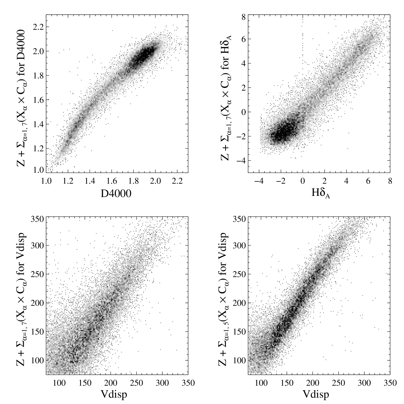
Figure 8: The linear combinations of the PC coefficients predicted to provide the best representation of D4000, H$\delta_{A}$ and stellar velocity dispersion (see Section 3 for details) are plotted as a function of direct measurements of these quantities from the SDSS pipeline. 5 PCs are used for the bottom-right panel, while 7 PCs are used for the other three panels. The sample has been restricted to DR7 galaxies with spectral median S/N per pixel greater than 10.

4 Advantages of the Principal Component Method

In the previous section, we described our methodology for deriving a set of principal components from a library of model spectra, for decomposing real galaxy spectra into linear combinations of these components, and for estimating errors on the derived PC amplitudes. We also outlined a Bayesian technique for parameter estimation using the input model library. In this section, we will attempt to illustrate the power of our methodology by means of some scientific applications.

4.1 A robust method for stellar continuum fitting

To decompose the galaxy spectrum into the emission produced by ionized gas and that produced by stars, one usually attempts to fit a model that describes the stellar component of the galaxy and then one “subtracts” this model from the observed spectrum. Certain emission lines, for example H$\beta$, frequently occur in deep absorption troughs, particularly in early-type galaxies, so it is important that the model for the stellar continuum be as accurate as possible.

In previous work (Brinchmann et al., 2004; Tremonti et al., 2004), we employed a template-fitting procedure to model the stellar continuum. As described in section 3, instead of a set of templates, our new method finds the linear combination of PC eigenspectra that best fits the stellar continuum. In Figure 7, we show two examples of PCA fits to DR7 (left) and BOSS (right) galaxy spectra over the wavelength interval from 3700 to 5500Å. The upper panel shows the spectrum of a star forming galaxy with strong Balmer emission and small 4000 Å break, while the lower panel shows a typical early-type galaxy with strong stellar absorption features. The black lines are the normalized observations, the red lines show the best PCA fits, which are clearly very good.

4.2 Improvement in S/N over Lick Indices when using PC-based techniques

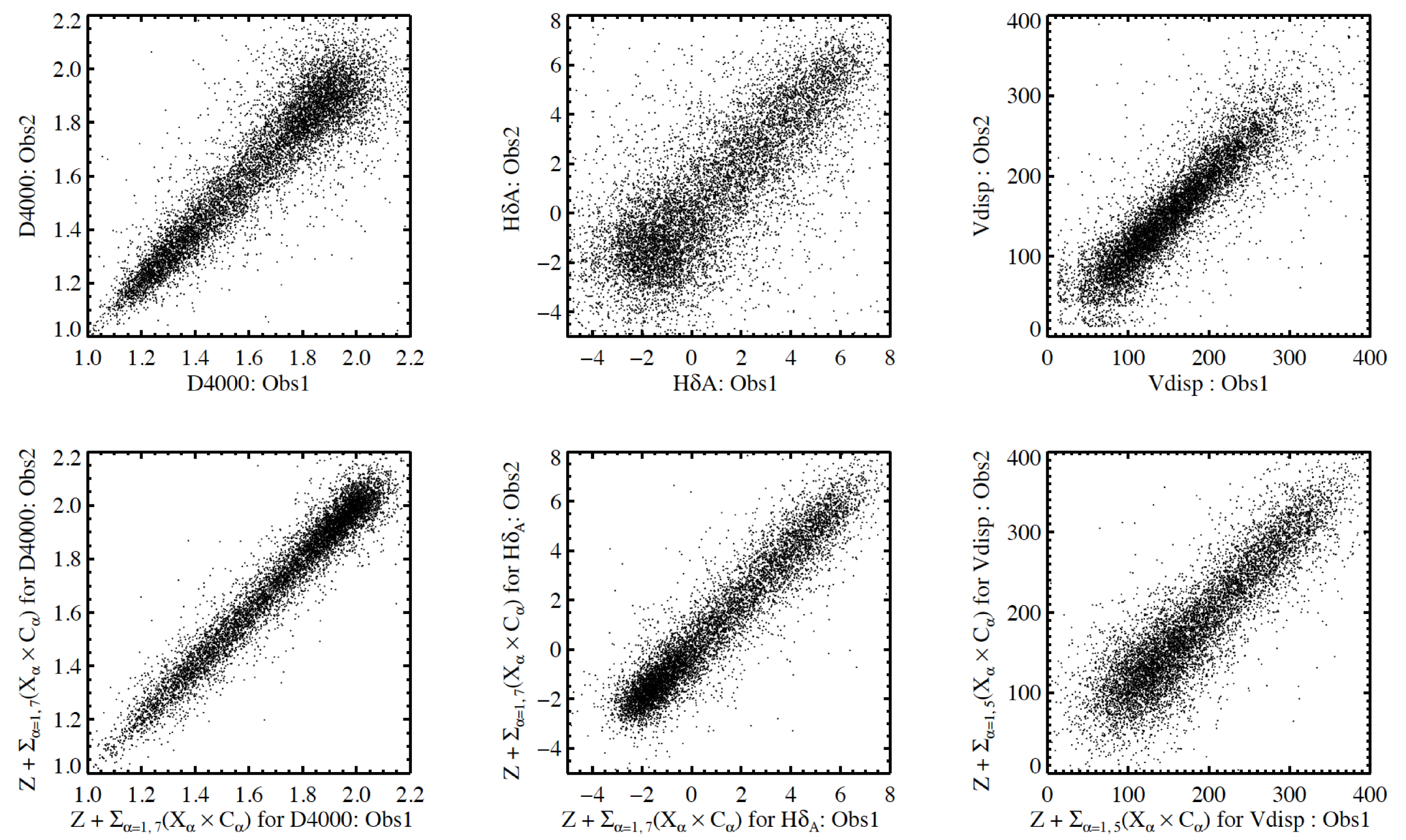
Figure 9: A sample of DR7 galaxies with two observations has been extracted from the SDSS database and measurements of D4000 (top-left) , H$\delta_{A}$ (top-middle) and $V_{\rm disp}$ (top-right) are plotted against each other in the top panel. The corresponding PC representations of these quantities are plotted against each other in the bottom panel.

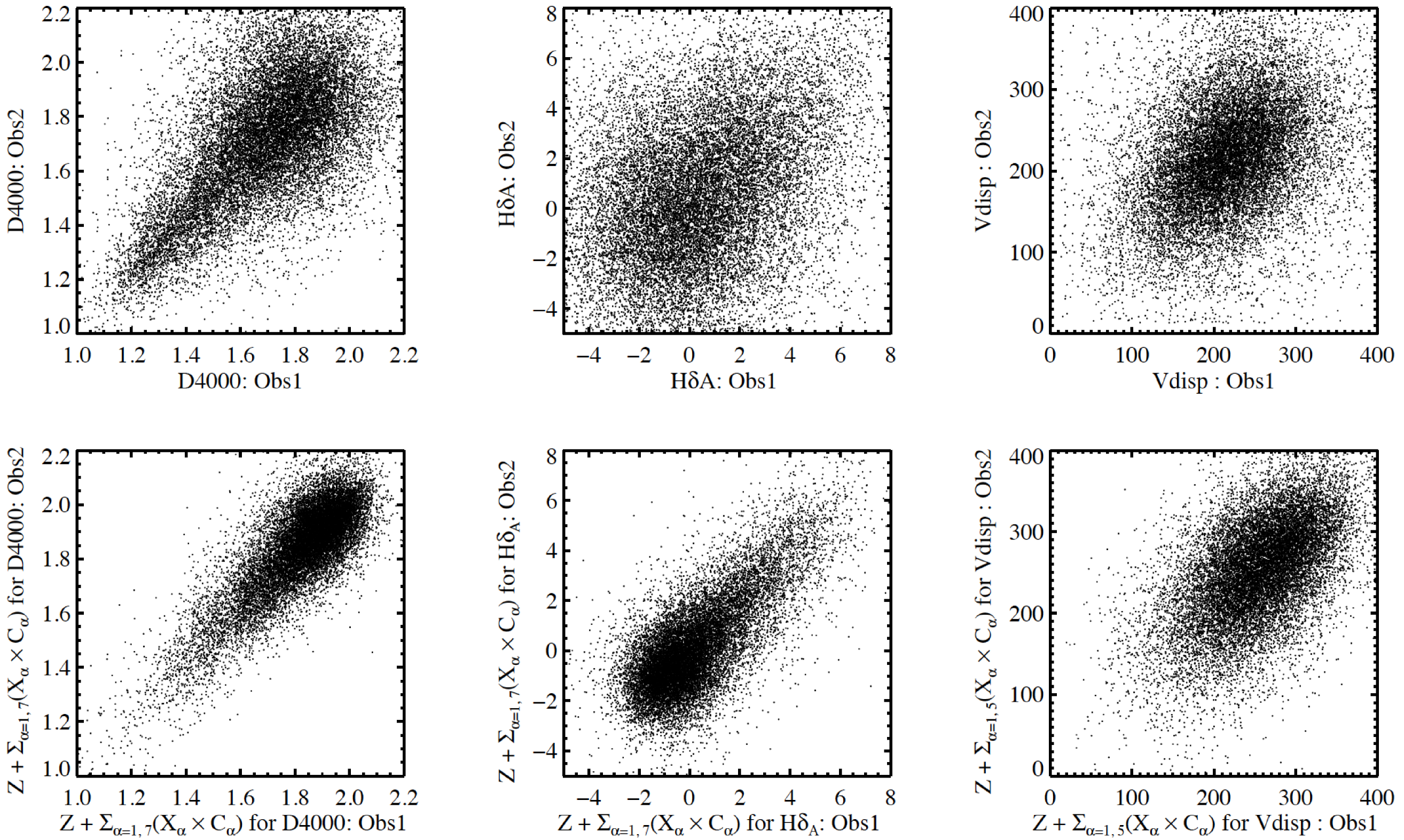
Figure 10: This figure is similar to Figure 9, except that results are shown for multiply-observed CMASS galaxies.

It is traditional to focus on specific stellar absorption features over a narrow wavelength interval when analyzing the ages and metallicities of the stellar populations of galaxies from their spectra. For galaxies with old stellar populations, the Lick/IDS system of $\sim$25 narrow-band indices is often used (Worthey, 1994; Worthey & Ottaviani, 1997; Gorgas et al., 1999). For actively star-forming galaxies, the 4000 Å break (Balogh et al., 1999) and Balmer absorption line features, such as the H$\delta_{A}$ index, provide important information about stellar age and recent star formation history (Kauffmann et al., 2003a). Finally, the velocity dispersion of the stars in the galaxy is traditionally estimated by comparing the width of stellar absorption features with those in unbroadened stellar templates (see Appendix B of Bernardi et al. 2003 for a review).

In Figure 3 of Section 3, we used model galaxy spectra to illustrate how narrow-band spectral indices such as D4000 and H$\delta_{A}$ could be “recovered” from appropriate linear combinations of the PCs. We also showed that the PCs could in principle be used to recover an estimate of stellar velocity dispersion. Figure 8 illustrates how well this works for real galaxy spectra. We compare $Z+\sum_{\alpha}(X_{\alpha}\times C_{\alpha})$ (using the $X_{\alpha}$ and $Z$ values in Table 1) with actual measurements of D4000, H$\delta_{A}$ and stellar velocity dispersion for a subset of galaxies drawn from the DR7 sample (note that these measurements are drawn from the MPA/JHU database). Since the purpose of this figure is to illustrate how well the recovery of traditional Lick indices and stellar velocity dispersion estimates is able to work in principle, we only plot galaxies with spectra where the median S/N per pixel is greater than 10.

We obtain very tight correlations between the appropriate linear combinations $Z+\sum_{\alpha}(X_{\alpha}\times C_{\alpha})$ and both D4000 and H$\delta_{A}$. We were not able to recover a good correlation with the velocity dispersion from the SDSS pipeline unless we reduced the number of PC components from 7 to 5. As illustrated in Figure 4, PC₆ should in principle contribute significantly to our estimate of $V_{\rm disp}$. The increase in scatter when using seven PCs instead of five is attributable to the fact that there are large uncertainties in measuring PC₆ even for spectra with S/N per pixel greater than 10. Below, we will always use just 5 PCs when estimating velocity dispersions, but 7 PCs when estimating all other quantities.

We now demonstrate that $Z+\sum_{\alpha}(X_{\alpha}\times C_{\alpha})$ has higher signal-to-noise ratio than the direct measurements of D4000, H$\delta_{A}$ and velocity dispersion for typical galaxy spectra drawn from the DR7 and CMASS samples. As we will show, the improvement is most striking for the low S/N CMASS spectra. The upper panel of Figure 9 illustrates the scatter obtained between the directly measured values of D4000, H$\delta_{A}$, and velocity dispersion for two different observations of the same galaxy in DR7. The bottom panel shows the same format for the corresponding $Z+\sum_{\alpha}(X_{\alpha}\times C_{\alpha})$ representation of the same quantities. Figure 10 displays the same comparison based on repeat observations of CMASS galaxies; note that for this sample, $>85\%$ galaxies have a median S/N per pixel below 4. The improvement in S/N exhibited by the PC representations of D4000 and H$\delta_{A}$ are highly significant both for the DR7 galaxies and the CMASS galaxies. The improvement in the PC-based velocity dispersion estimate is only obvious for the low S/N CMASS sample.

5 Application of the Principal Component Method to Stellar Mass Estimation

The application we wish to highlight in this paper (more applications will follow in subsequent work) is the derivation of robust PCA-based stellar masses for galaxies from the DR7 and CMASS samples. For each sample, two sets of stellar masses are estimated: the stellar mass measured within the fiber and the total mass. In the case of DR7, the masses are calculated by multiplying $M_{*}/L_{z}$ by the $z$-band luminosity measured within the $3^{\prime\prime}$ SDSS-I spectrograph fiber aperture, or by the luminosity $L_{z}$ derived from the SDSS $z$-band “model” magnitude. For the CMASS sample, $M_{*}/L_{i}$ is multiplied by the $i$-band luminosity measured within a $2^{\prime\prime}$ diameter aperture matched to the smaller BOSS spectrograph fibers, or by the $i$-band luminosity $L_{i}$ derived from the SDSS $i$-band “cmodel” magnitudes. We note that “model” and “cmodel” magnitudes are close to equivalent for DR7 galaxies, but diverge at the fainter magnitudes of the CMASS sample. In general “model” magnitudes are recommended for characterizing the colors of extended objects, since the light is measured consistently through the same aperture in all bands, while the “cmodel’ magnitudes provide a more reliable estimate of the total flux from the galaxy that accounts for the effects of local seeing.

Before we present science results using PCA-based masses, we compare them with the photometrically-derived ones. For the DR7 sample, photometric masses are given in the MPA/JHU catalog and derived from the $u,g,r,i,z$ broad-band photometry as described in §2.1. For the BOSS sample, we do not have an independent set of photometrically-derived stellar masses for comparison. However, we estimate the stellar mass-to-light ratio $M_{*}(g,r,i,z)/L_{i}$ by fitting the observed $g,r,i,z$-band fiber fluxes using the same model library. We have not included the $u$-band in our fits, because the CMASS galaxies are faint in the $u$-band and the errors are large. In order to avoid any uncertainties due to aperture effects, we use fiber masses in this whole section.

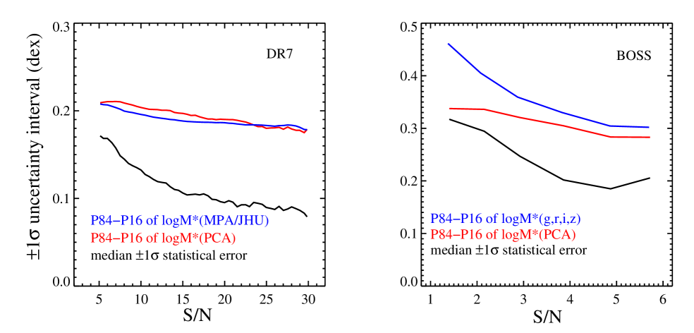
Figure 11: The $\pm 1\sigma$ uncertainty interval in the logarithm of the stellar mass for DR7 (left) and CMASS (right) galaxies. Results are plotted as a function of the median S/N per pixel in the spectrum. In both panels, red lines show the median value of P84 $-$ P16 as a function of S/N; P84 and P16 are the 84th and 16th percentiles of the cumulative PDF of the PCA-based stellar mass estimate ${\rm log}M_{*}({\rm PCA})$ for each galaxy. Blue lines show the same quantity for the photometrically-derived stellar masses. The black lines are the median $\pm 1\sigma$ statistical errors derived from repeat observations.

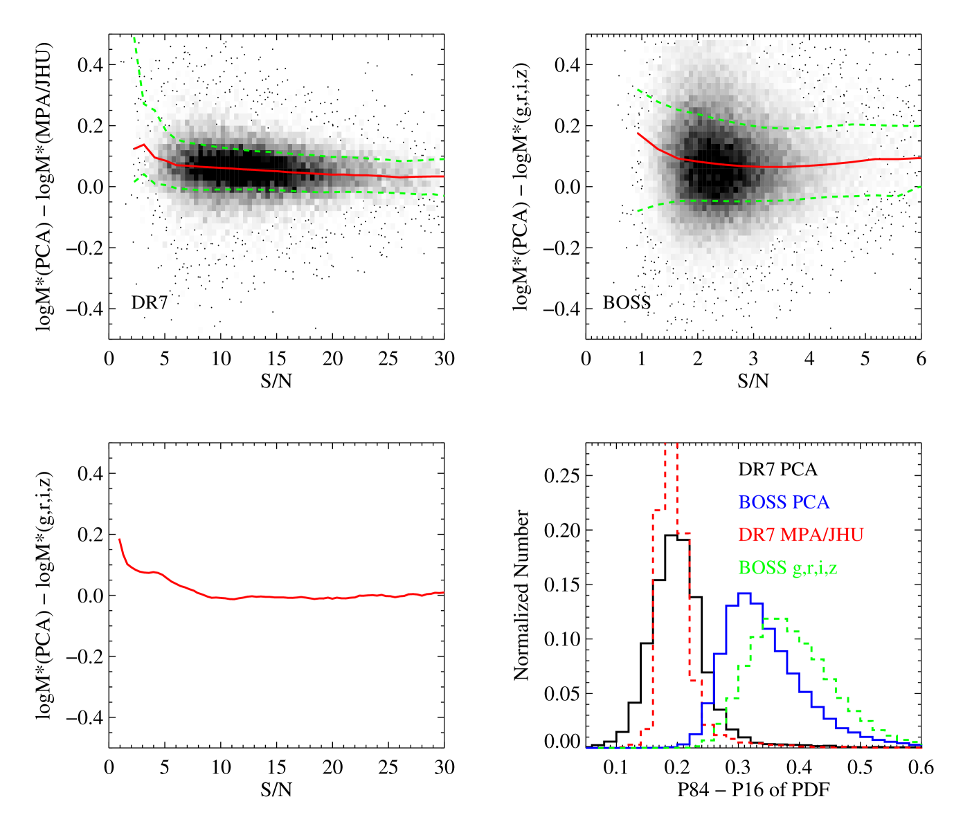
Figure 12: The difference between our PCA-based stellar masses and those derived from broad-band photometry is plotted as a function of median S/N per pixel for DR7 galaxies (top-left) and for the CMASS sample (top-right). In both panels, the over-plotted red line is the median, the two green dashed lines show the 68% spread. Bottom-left: the median discrepancy between PCA-based stellar masses and those derived from $g,r,i,z$-band photometry as a function of spectral median S/N per pixel for the combined DR7 and CMASS samples. Bottom-right: histograms of the distribution of (P86 $-$ P14), where P84 and P16 are the 84th and 16th percentile points of the cumulative PDF of the stellar mass estimated (derived using PCs) for DR7 galaxies (black) and for CMASS galaxies (blue). Red and green dashed lines show histograms of the same quantity for stellar masses derived from photometry for DR7 and BOSS, respectively.

Figure 11 shows the $\pm 1\sigma$ uncertainty interval in $\log M_{*}$ for DR7 (left) and CMASS (right) galaxies. Results are plotted as a function of the median S/N per pixel in the spectrum. In both panels, the red lines show the median values of P84 $-$ P16 in each S/N bin; P84 and P16 are the 84th and 16th percentiles of the cumulative PDF of our PCA-based stellar mass estimate ${\rm log}M_{*}({\rm PCA})$. The blue lines track the same quantity for the photometrically-derived stellar mass estimates. The black lines represent the $\pm 1\sigma$ scatter in the $\log M_{*}$ estimates derived from repeat observations. For DR7 galaxies, the errors on the stellar mass are virtually identical when using PCA to fit the spectra, or when fitting to the photometry. For BOSS, the PCA method yields significantly smaller errors, particularly at low S/N. This behaviour is expected, because the BOSS galaxies with low S/N spectra are faint galaxies where photometric errors tend to be large.

We also note that P84 $-$ P16 of ${\rm log}M_{*}({\rm PCA})$ is in general larger than the median $\pm 1\sigma$ statistical scatter in $\log M_{*}$ derived from repeat observations. This feature arises because the latter is only a measure of the error on $\log M_{*}$ due to noise in the spectra; the former accounts for both noise and the fact that different model galaxies with different $M_{*}/L$ values occupy the same region of PC-space.

5.1 Comparison with photometrically-derived stellar masses

In Figure 12, we compare the PCA-based stellar masses with the photometric masses. The top-left panel of Figure 12 shows the difference between ${\rm log}M_{*}({\rm PCA})$ and ${\rm log}M_{*}({\rm MPA/JHU})$ as a function of S/N for DR7 galaxies. The red line is the median, the two green dashed lines show the 68 percentile spread. There is a systematic $\sim$0.05 dex offset between the two mass estimates, but the scatter is quite small ($<\pm 0.1$ dex at S/N $>10$). The offset of our PC-based stellar mass estimates to slightly higher values is expected given that our model library includes truncated SFHs and a smaller fraction of galaxies with recent bursts (10% instead of 50%). In the next section, we will discuss how different assumptions about the mixture of SFHs in the model library influence our stellar mass estimates.

The top-right panel of Figure 12 shows the difference between ${\rm log}M_{*}({\rm PCA})$ and ${\rm log}M_{*}(g,r,i,z)$ for CMASS galaxies. Although these two sets of stellar masses are derived using exactly the same model library, the PCA-based stellar masses are typically 0.08 dex higher than the ones estimated using the $g,r,i,z$-band photometry. In the bottom-left panel of this figure, we plot the median discrepancy as a function of spectral median S/N per pixel for the combined DR7 and CMASS samples, finding that the offset disappears when S/N $>$ 8. We conclude that in the limit of high S/N, the two methods of estimating stellar mass yield exactly the same results.

Finally, the bottom-right panel of Figure 12 shows the distribution of the $\pm 1\sigma$ errors (i.e. P84 $-$ P16) for our different sets of stellar mass estimates. Black and blue histograms are for the PC-based stellar masses for DR7 and CMASS. The dashed red and green histograms show error distributions for the stellar masses derived from the photometry. For DR7 galaxies, the $\pm 1\sigma$ uncertainties on the PCA-based and photometry-based masses peak at nearly the same value, with the DR7 photometric measurements having slightly less dispersion. However, for the CMASS sample, the errors on the photometry-based masses are on average $\sim$0.05 dex larger than those derived using Principal Components, again reflecting the fact that the photometric errors are larger for this sample.

5.2 Dependence of our stellar mass estimates on the input parameters of the model library

In this section, we study the sensitivity of our stellar mass estimates to the input parameters of the model library. We change the input SFHs, dust extinction values and metallicity distributions in the model library one at a time, and quantify the effect on the stellar masses.

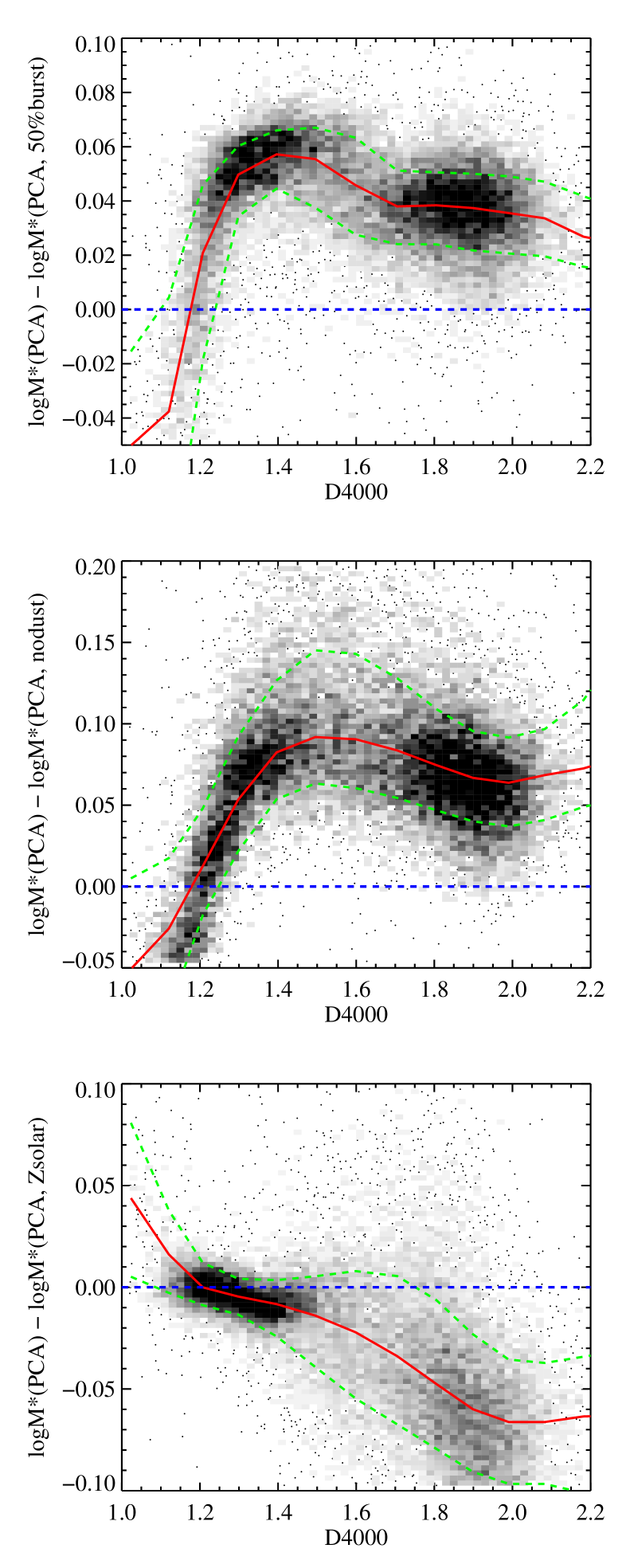
Figure 13: The dependence of stellar masses on the input parameters of the model library. Top panel: the difference between stellar masses based on the standard library and a library with a 50% burst fraction; middle panel: the difference between stellar masses based on the standard library and a library with no dust extinction; bottom panel: the difference between stellar masses based on the standard library and a solar metallicity library. In all these plots, the red lines denote the median of $\Delta{\rm log}M_{*}$, and the two green dashed lines show the 68% spread.

5.2.1 Star formation histories

In the previous section, we explained the 0.05 dex systematic difference between $M_{*}$(PCA) and $M_{*}$(MPA/JHU) as a consequence of the different SFHs used in generating the libraries. To confirm this idea, we have generated a new set of stellar mass estimates using a library in which the burst fraction is increased from 10% to 50%. The top panel of Figure 13 shows the difference in the stellar mass estimates $\Delta{\rm log}M_{*}={\rm log}M_{*}({\rm PCA})-{\rm log}M_{*}({\rm PCA,50\%burst})$ as a function of D4000, where $M_{*}({\rm PCA,50\%burst})$ is the library with 50% burst fraction. Once again the red line in the top panel of Figure 13 shows the median value of $\Delta{\rm log}M_{*}$, while the two green dashed lines show the 68% spread. In the range of $1.4<D4000<2.2$, $\Delta{\rm log}M_{*}\sim 0.05$, consistent with the systematic offset found between our PC-based mass estimates and the photometrically derived ones for DR7 sample in §5.1. At lower values of D4000, galaxies are constrained to have formed a significant fraction of their stars recently, so the difference in the fraction of bursty galaxies in the library makes a much smaller difference to the results.

5.2.2 Dust extinction

To check how assumptions about dust extinction influence our stellar mass estimates, we generate a library without dust extinction. The middle panel of Figure 13 shows the difference $\Delta{\rm log}M_{*}={\rm log}M_{*}({\rm PCA})-{\rm log}M_{*}({\rm PCA,nodust})$ as a function of D4000. $\Delta{\rm log}M_{*}$ increases as a function of D4000 up to value of $\sim 0.08$ at D4000 $\sim 1.5$, and then remains approximately constant. The systematically smaller stellar mass-to-light ratios derived using the library with no dust extinction can be understood, because a smaller fraction of the optical light from the galaxy is assumed to be absorbed. If dust is not included in the models and D4000 is large, the fit is able to re-adjust to match with an older stellar population, which has higher mass-to-light ratio. At low D4000 values, the stellar population is more tightly constrained to be young, so the degeneracy is again less important.

5.2.3 Metallicity

To check how assumptions about metallicity influence our stellar mass estimates, we generate a library with only solar metallicity models. The bottom panel of Figure 13 show the difference $\Delta{\rm log}M_{*}={\rm log}M_{*}({\rm PCA})-{\rm log}M_{*}({\rm PCA,Zsolar})$ as a function of D4000. As can be seen, for the young populations (D4000 $<$1.5) the systematic effects induced by adopting incorrect metallicity assumptions are very small. For the older populations, the difference increases with D4000, which is indicative of the well-known age-metallicity degeneracy.

In summary, stellar mass estimates are most strongly affected by assumptions about dust extinction, but also by the SFHs and metallicity of the model library galaxies. In all three cases, systematic offsets are of order 0.05$-$0.1 dex in $\log M_{*}$. Note we have not considered changes to the IMF. To convert our Kroupa (2001) stellar masses to a Salpeter (1955) or Chabrier (2003) IMF, one should add 0.18 dex to or subtract 0.05 dex from the logarithm of stellar masses, respectively. We note, however, that the Salpeter (1955) IMF is disfavoured by dynamical $M_{*}/L$ estimates of elliptical galaxies (Cappellari et al., 2006).

5.3 The dependence of stellar masses on the assumed stellar population synthesis model

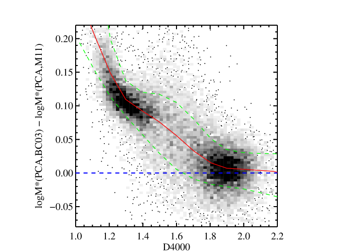
Figure 14: The difference in stellar masses derived from solar metallicity libraries based on BC03 and M11 models.

Kannappan & Gawiser (2007) compared photometrically-derived stellar masses based on BC03 and Maraston (2005) population synthesis models. These models are quite different in the optical due to the use of different stellar libraries. They found that BC03 models yield stellar mass estimates that are $\sim$1.3 times larger, even when no near-IR photometry is used in the fits.

In this section, we investigate systematic uncertainties that may arise in our PCA-based stellar mass estimates as a result of our choice of stellar population synthesis model. Maraston & Stromback (2011) present high spectral resolution stellar population models using the MILES stellar library (Sánchez-Blázquez et al., 2006) as input. The models have been extended with SSPs based on theoretical stellar libraries, which extend the wavelength coverage of the models into the ultra-violet.

We compare results at solar metallicity, where the stellar age coverage of the current version of the M11 model we are using is most reliable. Figure 14 shows the difference in the stellar masses estimated using these two libraries as a function of D4000. The strongest systematic discrepancy appears at young ages (low values of D4000), and decreases for older stellar populations. The offset of $\sim 0.12$, consistent with the result of Kannappan & Gawiser (2007), arises because the M11 models use Geneva tracks (Schaller et al., 1992; Meynet et al., 1994) to model stellar evolution, while the BC03 models make use of Padova tracks (Alongi et al., 1993; Bressan et al., 1993; Fagotto et al., 1994a, b; Girardi et al., 1996). In these tracks different assumptions are made regarding convective overshooting and the temperature and energetics of the Red Supergiant Phase, leading to a significantly redder supergiant phase in the M11 models.

We note that the prescription for stellar mass loss is somewhat different betwimeen BC03-models and Maraston-models, so we have used the BC03 mass loss prescriptions when performing the comparison shown in Figure 14.

6 Evolution of Massive Galaxies to Redshift 0.6

Figure 15 shows the distribution of total stellar masses based on the PCA method for the BOSS CMASS sample. As can be seen, the range of stellar masses spanned by this sample is rather narrow: $11\leq\log M_{*}\leq 12$. In the local Universe, galaxies in this stellar mass range are mainly “red and dead” systems with no ongoing star formation. Many reside in groups and clusters and have radio jets, which are believed to heat the surrounding gas, preventing it from cooling and forming stars (Boehringer et al., 1993; McNamara et al., 2000; Fabian et al., 2003; Best et al., 2005a, b, 2006; Bower et al., 2006; Croton et al., 2006). According to the currently popular “down-sizing” scenario for galaxy evolution, galaxies of this mass should have completed their star formation at very early epochs ($z>2$; Heavens et al., 2004; Thomas et al., 2005). They may subsequently grow through merging, but these merger events are believed to be largely dissipationless (i.e. “gas-free”; Naab et al., 2006; Bell et al., 2006; Scarlata et al., 2007; Kang et al., 2007). If this picture is correct, we would expect the stellar populations of very massive galaxies to evolve only “passively” over the redshift interval from 0.6 to 0. In this section, we check whether these expectations are correct.

Figure 15: The distribution of our PCA-based stellar masses for BOSS CMASS sample.

6.1 Fraction of massive galaxies with young stars

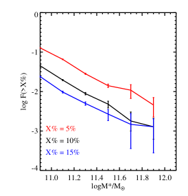
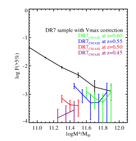
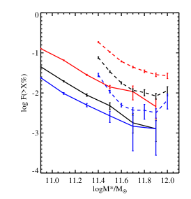
Figure 16: This figure shows the fraction of galaxies which have $>$ X% stars formed in the last Gyr as a function of stellar mass. Left panel: The red, black and blue lines show ${\rm log}F(>5\%)$, ${\rm log}F(>10\%)$ and ${\rm log}F(>15\%)$ for the DR7 sample. Middle panel: The purple, red, blue, green lines (they have been slightly displaced in the x-axis by minus 0.1, 0.05, 0.0, $-$0.05dex, respectively) are results for the redshifted DR7 samples at $z=0.45,0.5,0.55$ and 0.6, after application of the CMASS color cuts, compared to the results obtained for the unredshifted DR7 sample (in black). Right panel: The dashed lines show log$F(>5\%)$, log$F(>10\%)$ and log$F(>15\%)$ for CMASS sample with $z>0.54$ and $\log M_{*}>11.4$; this is a lower limit since the $d_{\perp}>0.55$ constraint deletes some blue galaxies from the sample. Solid lines show the DR7 results for reference.

Our PC-decomposition technique can isolate galaxies which have had more than a few percent of their stellar masses formed in the last Gyr (see panel (h) of Figure 3). We explore the robustness of the SFHs derived by the PCA method in the Appendix. In this section, we define parameters $F(>5\%)$, $F(>10\%)$, and $F(>15\%)$, which represent the fraction of galaxies in which more than 5, 10 and 15% of the stellar mass was formed in the last Gyr, respectively. Using DR7 and BOSS data, we study how these fractions have evolved since $z\sim 0.6$ for galaxies more massive than $\sim 2\times 10^{11}M_{\odot}$.

Starting from the DR7 Main galaxy sample, we construct a magnitude-limited sample of galaxies with $14.5<r<17.6$ and redshifts in the range $0.055<z<0.3$. We also limit the sample to galaxies with ZWARNING = 0 and SPECPRIMARY =1 to eliminate repeat observations and potential redshift errors. These restrictions result in a final DR7 sample of $\sim$430,000 galaxies. For each observed galaxy $i$, we define the quantity $z_{{\rm min},i}$ and $z_{{\rm max},i}$ to be the minimum and maximum redshift at which the galaxy would satisfy the apparent $r$-band magnitude limit. Evolutionary and K-corrections are included in this calculation (Li et al., 2007; Li & White, 2009). This allows us to define $V_{{\rm max},i}$ for the galaxy as the total comoving volume of the survey between $z1$ and $z2$, where $z1$ is the maximum of $z_{{\rm min},i}$ and 0.055, and $z2$ is the minimum of $z_{{\rm max},i}$ and $0.3$. $F_{*}>X\%$ can then be estimated as

$$F(>X\%)=\frac{\sum_{i=1,N_{\rm act}}(V_{{\rm max},i})^{-1}}{\sum_{j=1,N_{\rm all}}(V_{{\rm max},j})^{-1}},$$ (15)

where the sum on the numerator extends over $N_{\rm act}$, the number of galaxies in a given stellar mass bin that have formed more than X% of their stars in the last Gyr, while the sum on the denominator extends over $N_{\rm all}$, the total number of galaxies in the same mass bin.

The red, black and blue lines in the left panel of Figure 16 show ${\rm log}F(>5\%)$, ${\rm log}F(>10\%)$ and ${\rm log}F(>15\%)$ as a function of stellar mass for the DR7 sample (errors are derived from boot-strapping). As can be seen, all three fractions decrease strongly and monotonically with increasing stellar mass. At all stellar masses, there are 10 times more galaxies that have formed more than 5% of their stars over the last Gyr, compared to the number that have formed more than 15% of their stars in the last Gyr.

Before comparing these results with corresponding values of $F$ for CMASS galaxies at $z\sim 0.6$, we note that CMASS sample is not a simple magnitude-limited sample. There is a $d_{\perp}>0.55$ color cut, which means that blue galaxies will be lost from the survey, particularly at the lower redshift end. This means that the fraction of actively star-forming galaxies that we compute for the CMASS galaxies represents a lower limit to the true value.

Because we do not know the underlying relation between color and stellar mass for galaxies with $M_{*}>2\times 10^{11}M_{\odot}$ at $z\sim 0.55$ (existing surveys do not extend over wide enough areas to sample large numbers of very massive galaxies), it is difficult to correct for any missing blue galaxies. In order to provide a more quantitative idea of the degree to which the $d_{\perp}>0.55$ cut might affect our estimates of the fraction of galaxies with recent star formation, we use the K-correct code (Blanton & Roweis, 2007) to predict the colors of galaxies in the DR7 sample at redshifts $z=0.45,0.5,0.55$ and $0.6$. At each redshift, we select objects that pass the CMASS target selection criteria. In addition, we define a redshift-dependent lower stellar mass limit ${\rm log}M_{*}^{\rm lim}/M_{\odot}=2.0\times z+10.35$, so that a passively-evolving galaxy at redshift $z$ with stellar mass $M_{*}>M_{*}^{\rm lim}$ would pass all the target selection criteria in equation (1) (with the exception of $i_{\rm fiber2}<21.5$, which is more difficult to estimate unless one has a model for the structure of the galaxy).

The colored lines in the middle panel of Figure 16 show ${\rm log}F(>10\%)=N_{\rm act}/N_{\rm all}$ for the four redshifted DR7 samples (the purple, red, blue, green lines have been slightly displaced in the x-axis by minus 0.1, 0.05, 0.0, $-$0.05dex, respectively), compared to the results obtained for the unredshifted DR7 sample (in black) . As can be seen, the fraction of massive galaxies with recent star formation could be under-estimated by more than a order of magnitude at $z<0.55$. At higher redshifts, the fraction of actively star-forming galaxies that is missed is closer to a factor $\sim 2$. We therefore select a sub-sample of the CMASS galaxies with $0.54<z<0.7$ (0.54 is the median redshift of the CMASS sample) and log$M_{*}/M_{\odot}>11.4$ as the main high-redshift comparison sample for the DR7 massive galaxies.

In the right panel of Figure 16, the dashed lines show log$F(>5\%)$, log$F(>10\%)$ and log$F(>15\%)$ as a function of stellar mass for this sample. Solid lines show the DR7 results for reference. $z_{{\rm min},i}$ and $z_{{\rm max},i}$ values have been calculated for this sample by evaluating the minimum and maximum redshifts at which the galaxy would satisfy all the criteria in equation (1) except $i_{\rm fiber2}<21.5$. Evolutionary and K-corrections are included in this calculation. $V_{{\rm max},i}$ is calculated as the comoving volume of the survey between $z1$ and $z2$, where $z1$ is the maximum of $z_{{\rm min},i}$ and 0.54, and $z2$ is the minimum of $z_{{\rm max},i}$ and $0.7$.

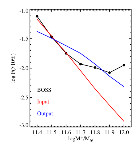
Figure 17: The black line reproduces the black dashed line in the right panel of Figure 16. The three low mass data points on this black line are fitted with a linear relation ${\rm log}F_{*}(>10\%)=-3\times{\rm log}M_{*}/M_{\odot}+33$. We randomly generate a sample of 1,000,000 galaxies with ${\rm log}M_{*}/M_{\odot}$ has a Gaussian distribution over the range of [11.1, 12.1] with a peak at $\sim$11.55 and 68% of them distributed over the range 11.37$-$11.73. We assign a value of $F_{*}$ to each galaxy so that the linear relation is reproduced on average (red line on the plot). We then add an error to each stellar mass using the error distribution of CMASS galaxies as a function of $M_{*}$. This mimic sample has a similar distribution in ${\rm log}M_{*}/M_{\odot}$ as our CMASS galaxies within $0.54<z<0.7$. We then recompute the relation between ${\rm log}F_{*}(>10\%)$ and stellar mass, the result is shown as the blue line.

One conclusion from Figure 16 is that the fraction of actively star-forming galaxies with $\log M_{*}>11.4$ has evolved strongly since a redshift of $\sim 0.6$. This result is not surprising. The evolution of the dependence of star formation on galaxy stellar mass has been studied using data from other deep surveys (e.g., Zheng et al., 2007; Chen et al., 2009; Karim et al., 2011) and, in general, the claim was been that the rate of decline in cosmic SFR with redshift is the same at all stellar masses. None of these previous surveys, however, have extended to stellar masses as high as $10^{12}M_{\odot}$. In the BOSS data, we find the striking result that the fraction of actively star formation galaxies flattens above a stellar mass of $10^{11.6}M_{\odot}$ at $z\sim 0.6$. At the largest stellar masses, therefore, the evolution in the fraction of star-forming galaxies from $z\sim 0.6$ to the present-day is even more dramatic, reaching a factor of $\sim 10$ at $\log M_{*}\sim 12$. We emphasize once again that these numbers represent lower limits on the evolution, because of the incompleteness issues described above.

Because the uncertainties in the BOSS stellar masses are larger than our bin size, we have done tests to explore whether “smearing” of the true stellar mass distribution could produce the observed flattening. In Figure 17, the black line reproduces the black dashed line in the right panel of Figure 16. We fit the three low mass data points with a linear relation ${\rm log}F_{*}(>10\%)=-3\times{\rm log}M_{*}/M_{\odot}+33$. We randomly generate a sample of 1,000,000 galaxies with ${\rm log}M_{*}/M_{\odot}$ has a Gaussian distribution over the range of [11.1, 12.1] with a peak at $\sim$11.55 and 68% of them distributed over the range 11.37$-$11.73. We assign a value of $F_{*}$ to each galaxy so that the linear relation is reproduced on average (red line on the plot). We add an error to each stellar mass using the error distribution of CMASS galaxies as a function of $M_{*}$. This mimic sample has a similar distribution in ${\rm log}M_{*}/M_{\odot}$ as our CMASS galaxies within $0.54<z<0.7$. We then recompute the relation between ${\rm log}F_{*}(>10\%)$ and stellar mass and the result is shown as the blue line. The main conclusion from Figure 17 is that errors will act to flatten the trend, but this is a small effect compared to what is seen in the data. Smearing by errors also cannot explain the characteristic mass scale of $\log M_{*}=11.6$ where the flattening appears to set in.

6.2 AGN and star formation in massive galaxies

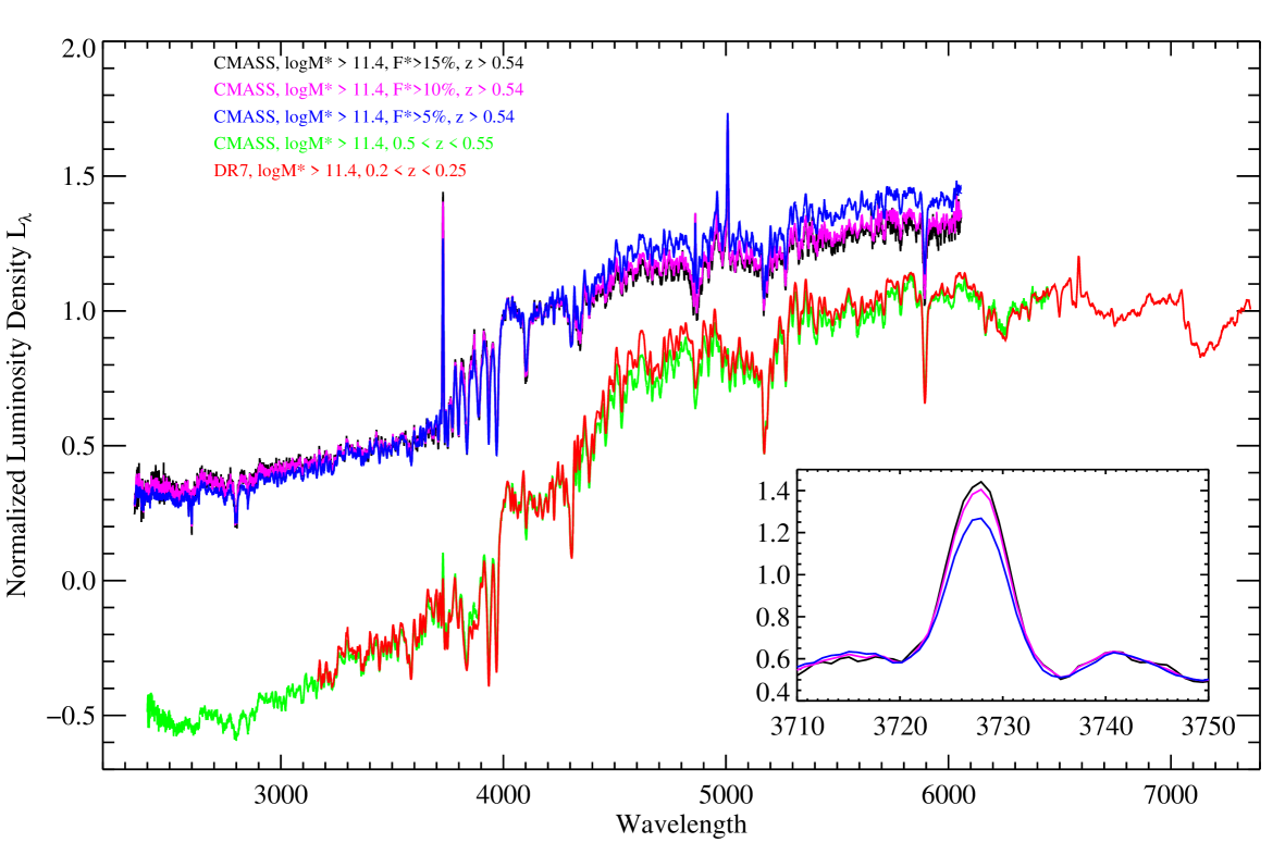
Figure 18: The black, magenta and blue spectra represent the stacks of galaxies with $F_{*}>15\%$, $F_{*}>10\%$, and $F_{*}>5\%$ in CMASS sample, respectively. The red spectrum is the stack of “inactive” ($F_{*}<10\%$) DR7 galaxies with log$M_{*}/M_{\odot}>11.4,0.2<z<0.25$, the green spectrum shows its CMASS twin sample which has exactly the same mass distribution and $F_{*}<10\%,0.5<z<0.55$. The insert drawing highlights the region near the [O ii] line.

The CMASS galaxies are massive (log$M_{*}/M_{\odot}>10^{11.2}$) and predominantly bulge-dominated (, Masters et al.2011), therefore it is likely that they host supermassive black holes. In bulge-dominated galaxies where star-formation is ongoing, the black holes are usually accreting actively (Heckman et al., 2004; Kauffmann & Heckman, 2009). We now turn to examining the black hole accretion rate using the [O iii]$\lambda 5007$ line as an indicator of the AGN’s bolometric luminosity. Because the individual spectra are noisy, we average them to create high-S/N composites.

We present stacked spectra of CMASS galaxies with $F_{*}>X\%$ ($X\%$ = 5%, 10% or 15%), log$M_{*}/M_{\odot}>11.4,z>0.54$. The galaxy spectra are first corrected for foreground Galactic attenuation using the dust maps of Schlegel et al. (1998), transformed from vacuum wavelengths to air, from flux densities to luminosity densities, and shifted to the rest frame using the redshift determined by the BOSS pipeline. The rest-frame spectra are averaged with weight $1/V_{\rm max}$ (Note that the weight of the bad pixels identified in the SDSS mask array is set to zero). Finally, we normalize the stacked spectra by their mean luminosity in the wavelength range 4000$-$4080Å. The black, magenta and blue spectra in Figure 18 represent the normalized stacks of CMASS galaxies with $F_{*}>15\%$, $F_{*}>10\%$, and $F_{*}>5\%$, respectively. As expected, the [O ii] flux increases for larger values of $X$ and the spectra are also bluer.

In the following, we will concentrate on the stack with $F_{*}>10\%$. In order to quantify how AGN contribute to the line emission, we have selected DR7 galaxies with similar values of D4000, H$\delta_{A}$, log([O iii]/H$\beta$), log([O ii]/H$\beta$). When we combine the spectra of these “matched” DR7 galaxies, we find log([N ii]/H$\alpha$) $\approx-0.5$. log([O iii]/H$\beta$) is measured directly from the CMASS stack and is $\approx 0.2$. This implies that around half of the [O iii] luminosity in the stack is contributed by AGNs (Kauffmann et al., 2003b; Kauffmann & Heckman, 2009). We fit the stacked CMASS spectrum as a non-negative linear combination of single stellar population models, with dust attenuation modeled as an additional free parameter (Brinchmann et al., 2004; Tremonti et al., 2004). This fit yields a continuum $V$-band dust extinction value of 1.76. Taking a mean bolometric correction to the extinction-corrected [O iii] of 600 (Kauffmann & Heckman, 2009), and assuming that half of the [O iii] emission is coming from the AGNs, we find $L/L_{\rm Edd}\approx 0.01$, where $L_{\rm Edd}=1.38\times 10^{38}M_{\rm BH}/M_{\odot}$ is the Eddington luminosity and $M_{\rm BH}$ is estimated from the median value of the velocity dispersions of the galaxies that go into the stack using the formula given in Graham et al. (2011) .

We have also cross-matched the BOSS and FIRST surveys, and found that $\sim$2.4%CMASS galaxies have FIRST detections. The typical $i$-band magnitude and mass of this radio loud sample are 19.6 and $10^{11.6}M_{\odot}$, respectively. For this radio-detected sample, we construct a control sample matched in redshift, stellar mass, and velocity dispersion which are located in the FIRST survey area but lack radio detections. Interestingly, the fraction of galaxies with recent star formation ($F_{*}>10\%$) is 2$-$2.5 times smaller in the radio-loud sub-sample than for the controls. We will study the difference between radio-loud and radio-quiet CMASS galaxies in more detail in future work.

The red spectrum in Figure 18 is a stack of DR7 galaxies with $F_{*}<10\%$, log$M_{*}/M_{\odot}>11.4$ and $0.2<z<0.25$. In order to make a fair comparison between DR7 and BOSS “inactive” galaxies, we construct a twin sample from CMASS galaxies in the redshift range $0.5-0.55$, which has exactly the same stellar mass distribution and $F_{*}<10\%$. The stacked spectrum of this twin sample is shown in green. (Note that the red and green spectra have both been shifted down by 0.7 from the other three spectra. The stacks are generated in the same way as the “active” star forming galaxies except we use an equal weight rather than $1/V_{\rm max}$). There is no apparent difference in the spectral shape and absorption line features of the stacks of DR7 and BOSS “inactive” galaxies.

In summary, we conclude that at $z\sim 0.6$ at least 2% of very massive galaxies have formed more than 10% of their stars in the last Gyr and nearly 10% have formed more than 5% of their stars over this period. We note that for a galaxy with $M_{*}\sim 10^{12}M_{\odot}$ to be counted as a member of the $F*>10\%$ “class”, it must have processed more than $10^{11}M_{\odot}$ of gas over the last Gyr or so, i.e. 6$-$8 times as much gas as contained in the Milky Way! If this gas is in molecular form, it should be easily detectable at $z\sim 0.6$. More detailed studies of these objects will reveal important insights into the physical processes that govern the evolution of massive galaxies at late times. Kaviraj et al. (2008) studied recent star formation in massive galaxies at $z\sim$ 0.6 using rest-frame UV data, and found young stars at levels of a few percent by mass fraction. Based on a strong correspondence between the presence of star formation (traced by UV colours) and the presence of morphological disturbances, Kaviraj et al. (2011) suggested the star formation is merger-driven. The major merger rate at late epochs ($z<1$) is predicted to be too low to produce the observed number of disturbed LRGs, so the authors invoked minor mergers as an alternative machanism. Future kinematic studies of larger sample of such galaxies would help test this hypothesis.

Appendix

Here we explore the robustness of the SFHs that we infer. Our analysis is based on restframe optical wavelengths which are contain a large contribution from intermediate age stars; therefore our code does best at recovering the SFR averaged over the last Gyr. In contrast, commonly used SFR tracers such as H$\alpha$, the far-ultraviolet, and the far-infrared trace star formation on timescales of $\sim$10$-$100 Myr (Kennicutt, 1998).

The recovery of galaxy star formation histories from integrated spectra is a difficult problem due to well-known degeneracies between age, metallicity, and dust attenuation. We explore the effect of these degeneracies on our SFR estimates in two ways: a) We generate synthetic data where the input parameters are well known and test the ability of our PCA-based algorithm to recover the true SFR. b) We use the real data to test whether our PCA-based SFR estimates give answers that are consistent with SFR derived from nebular emission lines. In the real universe there are strong correlations between SFR, stellar mass, metallicity, and dust attenuation (c.f., Brinchmann et al., 2004; Tremonti et al., 2004; Gallazzi et al., 2005; Asari et al., 2007). To ensure that our suite of test models reflected these parameter correlations, we used DR7 galaxies to define the input parameters of our model. We randomly selected 1000 SDSS DR7 star forming galaxies and tabulated their $M_{*}/L$ ratio, $V$-band dust attenuation of young stars ($\tau_{V}=A_{V}/1.086$), nebular metallicity, and SFR/$M_{*}$ from the MPA/JHU catalog. (The dust attenuation, metallicity, and SFR have been estimated from the nebular lines (Brinchmann et al., 2004). We assume that the stellar metallicity, $Z_{*}$, is 0.4 dex lower than the nebular metallicity, as found by Gallazzi et al. 2005.) For each galaxy we identified all the models in our library that were within $\pm$0.1 dex in log$(M_{*}/L)$, log(SFR/$M_{*}$), $Z_{*}$, and $\tau_{V}$, and we randomly selected 5 models from this subset. We used the error array of the SDSS spectrum to add realistic random errors to each of the model spectra. We then applied our PCA analysis to the $\sim$5000 simulated spectra and estimated $F_{*}$. In the top panel of Figure 19 we compare the input and output values of log$F_{*}$ as a function of stellar mass and dust attenuation for our simulated DR7 galaxies. In the lower panel we show the result of a similar exercise where we have substituted the error arrays of randomly selected BOSS galaxies to explore our ability to recover $F_{*}$ at the low S/N typical of BOSS. For the simulated DR7 and BOSS spectra, we recover $F_{*}$ to within $\pm 0.1$ and $\pm 0.2$ dex respectively. There is as a small systematic trend with dust attenuation that is evident in the noisier BOSS data, but this produces only a very weak systematic trend with stellar mass (less than 0.05 dex over two orders of magnitude in stellar mass). Thus, our PCA technique appears to accurately recover the SFR in the last Gry in the case where the input data is well represented by the models.

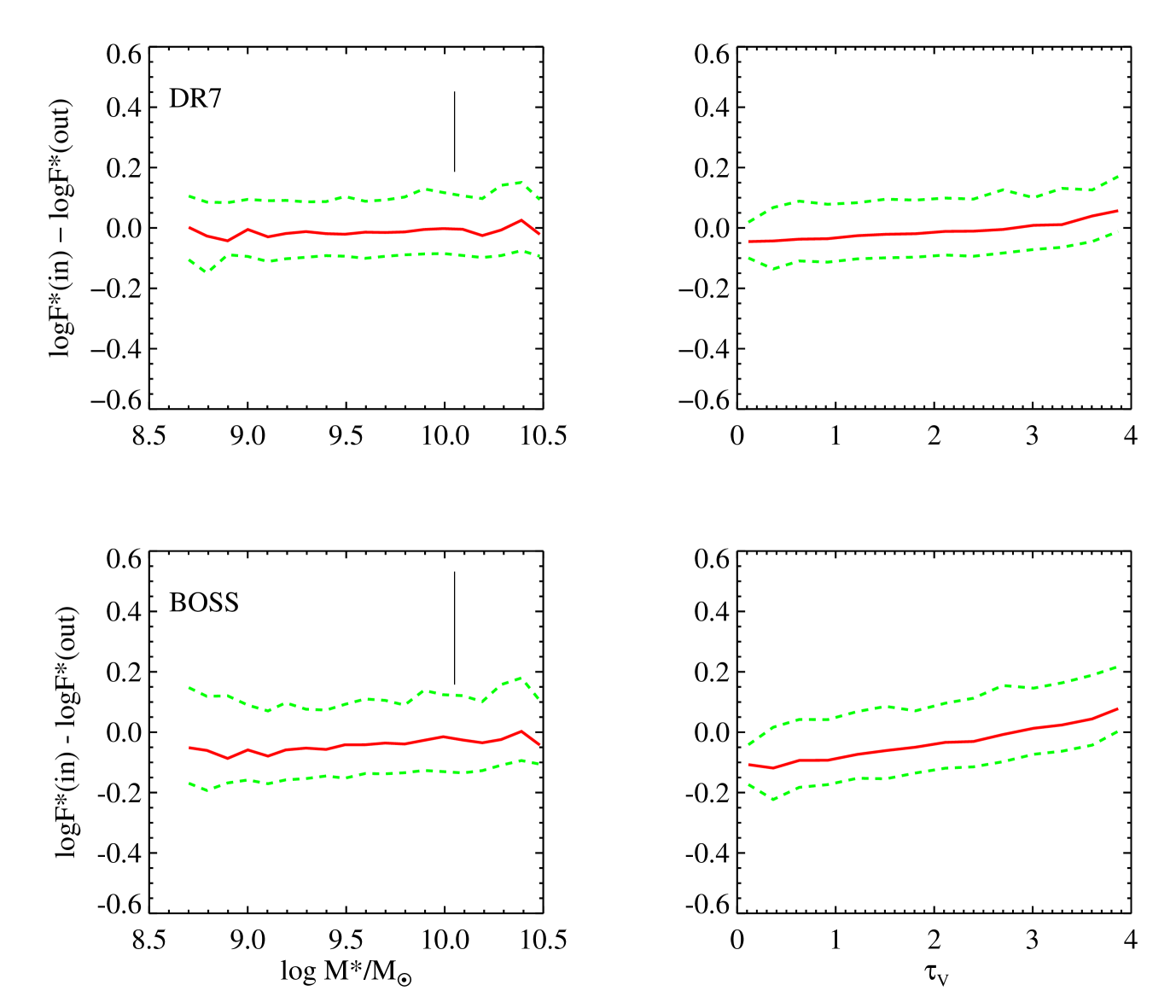
Figure 19: The difference between our input, $F_{*}({\rm in})$, and output, $F_{*}({\rm out})$ in tests using simulated data. As described in $\S$6, our suite of 5000 test spectra have values of SFR, $M_{*}$, $Z_{*}$, and $\tau_{V}$ drawn from DR7 star forming galaxies. The top panels and bottom panels show simulated DR7 and BOSS data while the left panels and right panels shows the log$F_{*}$ residuals versus stellar mass and $V$-band dust attenuation. The red solid line denotes the median and the green dashed lines enclose the 68% of the data points. A black error bar denotes the median $\pm 1\sigma$ error of the PCA-derived parameters. There is good agreement between the derived errors and the scatter in the input and output parameters, and only weak evidence for a systematic trend. This suggests that the PCA technique is relatively robust against degeneracies between age, dust, and metallicity and able to accurately recover the SFR in the last Gyr when the data is well represented by the model grid.

The next question is whether our choice of priors influences the derived value of $F_{*}$. We have done a variety of tests similar to those outlined in §5 and find that our derived SFHs are generally insensitive to changes in our input model grid. Not surprisingly, the parameter that is most important is the fraction of of galaxies with bursts in the input model library. In Figure 20, we plot $\Delta F_{*}=F_{*}({\rm PCA})-F_{*}({\rm PCA,50\%})$ as a function of $F_{*}({\rm PCA})$, where $F_{*}({\rm PCA})$ is our estimate of the fraction of young stars formed in the last Gyr using the fiducial model library and $F_{*}({\rm PCA,50\%})$ is the fraction estimated using the library with a 50% burst fraction. Although the difference in the two estimates is an increasing function of $F_{*}({\rm PCA})$, in percentage terms the two estimates give results that differ very little. Moreover, the bulk of our galaxies have very small values of $F_{*}$ where the difference is negligible.

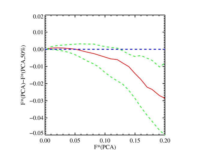
Figure 20: $\Delta F_{*}=F_{*}({\rm PCA})-F_{*}({\rm PCA,50\%})$ as a function of $F_{*}({\rm PCA})$, where $F_{*}({\rm PCA})$ is the fraction of stars formed in the last Gyr using the fiducial library, and $F_{*}({\rm PCA,50\%})$ is the fraction of stars formed in the last Gyr using the library with 50% burst fraction. The red lines denote the median value of $\Delta F_{*}$, and the two green dashed lines show the 68% spread in $\Delta F_{*}$.

Finally, for the DR7 star-forming galaxies, we directly compared the current SFR inferred from the nebular emission lines (Brinchmann et al., 2004) to our PCA-based estimates of the average SFR in the last Gry (SFR $=F_{*}\times M_{*}/10^{9}$ yr). The scatter at fixed stellar mass is 0.2 dex. Part of this may stem from real differences in the SFR over the timescales probed (10 Myr vs. 1 Gyr). Curiously, we find systematic trends with stellar mass and dust attenuation that are not present in our tests with simulated data (Fig. 19). For the real data, the PCA technique appears to underestimate the SFR inferred from extinction corrected H$\alpha$ by as much as 0.4 dex in the most massive (log$(M_{*}/M_{\sun})>10.8$) or dusty ($\tau_{V}>3$) galaxies. A systematic trend of this nature is difficult to explain by invoking star formation history differences as this would imply that all massive galaxies are in the midst of a burst at the current epoch. We note that similar discrepancies have been found in other works that compare information inferred from the restframe optical continuum and the nebular lines (c.f., Tanaka, 2011; Hoversten & Glazebrook, 2008; Gunawardhana et al., 2011). This suggests that commonly adopted model assumptions regarding dust attenuation or the initial mass function may be too simplistic. For instance, there is some evidence for a dust component associated with intermediate age stars (Eminian et al. 2008). Dust attenuation is also likely to be inhomogeneous within a given galaxy, and the net effect may not be well approximated by our two ‘effective’ global parameters, $\mu$ and $\tau_{V}$. The importance of dust inhomogeneities has been demonstrated in a study of 9 local galaxies using multiband photometry (Zibetti et al., 2009). Further exploration of the differences between spatially resolved and unresolved SFR and mass estimates will be possible with the next generation of integral field unit galaxy surveys (c.f., Sanchez et al., 2011). We defer a full analysis of the difference between PCA and nebular estimates of the SFR to future work. In $\S 7$ we will compare PCA-derived $F*$ values for DR7 and BOSS galaxies at fixed stellar mass. While the absolute values of $F*$ are somewhat uncertain, our analysis hinges on the relative differences which we believe to be robust.

References

- Abazajian et al. (2005) Abazajian K., Adelman-McCarthy J. K., Agüeros M. A., Allam S. S., Anderson K. S. J., Anderson S. F., Annis J., Bahcall N. A., et al. 2005, AJ, 129, 1755
- Abazajian et al. (2009) Abazajian K. N., Adelman-McCarthy J. K., Agüeros M. A., Allam S. S., Allende Prieto C., An D., Anderson K. S. J., Anderson S. F., Annis J., Bahcall N. A., et al. 2009, ApJS, 182, 543
- Aihara et al. (2011) Aihara H., Allende Prieto C., An D., Anderson S. F., Aubourg É., Balbinot E., Beers T. C., Berlind A. A., et al. 2011, ApJS, 193, 29
- Alongi et al. (1993) Alongi M., Bertelli G., Bressan A., Chiosi C., Fagotto F., Greggio L., Nasi E., 1993, A&AS, 97, 851
- Asari et al. (2007) Asari N. V., Cid Fernandes R., Stasińska G., Torres-Papaqui J. P., Mateus A., Sodré L., Schoenell W., Gomes J. M., 2007, MNRAS, 381, 263
- Balogh et al. (1999) Balogh M. L., Morris S. L., Yee H. K. C., Carlberg R. G., Ellingson E., 1999, ApJ, 527, 54
- Bell & de Jong (2001) Bell E. F., de Jong R. S., 2001, ApJ, 550, 212
- Bell et al. (2003) Bell E. F., McIntosh D. H., Katz N., Weinberg M. D., 2003, ApJS, 149, 289
- Bell et al. (2006) Bell E. F., Naab T., McIntosh D. H., Somerville R. S., Caldwell J. A. R., Barden M., Wolf C., Rix H.-W., et al. 2006, ApJ, 640, 241
- Benson et al. (2000) Benson A. J., Cole S., Frenk C. S., Baugh C. M., Lacey C. G., 2000, MNRAS, 311, 793
- Bernardi et al. (2003) Bernardi M., Sheth R. K., Annis J., Burles S., Eisenstein D. J., Finkbeiner D. P., Hogg D. W., Lupton R. H., et al. 2003, AJ, 125, 1817
- Best et al. (2006) Best P. N., Kaiser C. R., Heckman T. M., Kauffmann G., 2006, MNRAS, 368, L67
- Best et al. (2005a) Best P. N., Kauffmann G., Heckman T. M., Ivezić Ž., 2005a, MNRAS, 362, 9
- Best et al. (2005b) Best P. N., Kauffmann G., Heckman T. M., Brinchmann J., Charlot S., Ivezić Ž., White S. D. M., 2005b, MNRAS, 362, 25
- Blanton & Roweis (2007) Blanton M. R., Roweis S., 2007, AJ, 133, 734
- Boehringer et al. (1993) Boehringer H., Voges W., Fabian A. C., Edge A. C., Neumann D. M., 1993, MNRAS, 264, L25
- Borch et al. (2006) Borch A., Meisenheimer K., Bell E. F., Rix H., Wolf C., Dye S., Kleinheinrich M., Kovacs Z., Wisotzki L., 2006, A&A, 453, 869
- Bower et al. (2006) Bower R. G., Benson A. J., Malbon R., Helly J. C., Frenk C. S., Baugh C. M., Cole S., Lacey C. G., 2006, MNRAS, 370, 645
- Bressan et al. (1993) Bressan A., Fagotto F., Bertelli G., Chiosi C., 1993, A&AS, 100, 647
- Brinchmann et al. (2004) Brinchmann J., Charlot S., White S. D. M., Tremonti C., Kauffmann G., Heckman T., Brinkmann J., 2004, MNRAS, 351, 1151
- Bruzual & Charlot (2003) Bruzual G., Charlot S., 2003, MNRAS, 344, 1000
- Budavári et al. (2009) Budavári T., Wild V., Szalay A. S., Dobos L., Yip C.-W., 2009, MNRAS, 394, 1496
- Cappellari et al. (2006) Cappellari M., Bacon R., Bureau M., Damen M. C., Davies R. L., de Zeeuw P. T., Emsellem E., Falcón-Barroso J., et al. 2006, MNRAS, 366, 1126
- Chabrier (2003) Chabrier G., 2003, PASP, 115, 763
- Charlot & Fall (2000) Charlot S., Fall S. M., 2000, ApJ, 539, 718
- Chen et al. (2009) Chen Y.-M., Wild V., Kauffmann G., Blaizot J., Davis M., Noeske K., Wang J.-M., Willmer C., 2009, MNRAS, 393, 406
- Chen et al. (2010) Chen Y.-M., Tremonti C. A., Heckman T. M., Kauffmann G., Weiner B. J., Brinchmann J., Wang J., 2010, AJ, 140, 445
- Conroy et al. (2009) Conroy C., Gunn J. E., White M., 2009, ApJ, 699, 486
- Croton et al. (2006) Croton D. J., Springel V., White S. D. M., De Lucia G., Frenk C. S., Gao L., Jenkins A., Kauffmann G., Navarro J. F., Yoshida N., 2006, MNRAS, 365, 11
- Drory et al. (2004) Drory N., Bender R., Hopp U., 2004, ApJ, 616, L103
- Eisenstein et al. (2011) Eisenstein D. J., Weinberg D. H., Agol E., Aihara H., Allende Prieto C., Anderson S. F., Arns J. A., Aubourg E., Bailey S., Balbinot E., et al. 2011, ArXiv e-prints
- Eminian et al. (2008) Eminian C., Kauffmann G., Charlot S., Wild V., Bruzual G., Rettura A., Loveday J., 2008, MNRAS, 384, 930
- Fabian et al. (2003) Fabian A. C., Sanders J. S., Allen S. W., Crawford C. S., Iwasawa K., Johnstone R. M., Schmidt R. W., Taylor G. B., 2003, MNRAS, 344, L43
- Fagotto et al. (1994a) Fagotto F., Bressan A., Bertelli G., Chiosi C., 1994a, A&AS, 104, 365
- Fagotto et al. (1994b) Fagotto F., Bressan A., Bertelli G., Chiosi C., 1994b, A&AS, 105, 29
- Fukugita et al. (1996) Fukugita M., Ichikawa T., Gunn J. E., Doi M., Shimasaku K., Schneider D. P., 1996, AJ, 111, 1748
- Gallazzi et al. (2005) Gallazzi A., Charlot S., Brinchmann J., White S. D. M., Tremonti C. A., 2005, MNRAS, 362, 41
- Gallazzi et al. (2006) Gallazzi A., Charlot S., Brinchmann J., White S. D. M., 2006, MNRAS, 370, 1106
- Gallazzi & Bell (2009) Gallazzi A., Bell E. F., 2009, ApJS, 185, 253
- Girardi et al. (1996) Girardi L., Bressan A., Chiosi C., Bertelli G., Nasi E., 1996, A&AS, 117, 113
- Gorgas et al. (1999) Gorgas J., Cardiel N., Pedraz S., González J. J., 1999, A&AS, 139, 29
- Graham (2008) Graham A. W., 2008, ApJ, 680, 143
- Graham & Li (2009) Graham A. W., Li I.-h., 2009, ApJ, 698, 812
- Graham et al. (2011) Graham A. W., Onken C. A., Athanassoula E., Combes F., 2011, MNRAS, 412, 2211
- Gunawardhana et al. (2011) Gunawardhana M. L. P., Hopkins A. M., Sharp R. G., Brough S., Taylor E., Bland-Hawthorn J., Maraston C., Tuffs R. J., et al. 2011, MNRAS, 415, 1647
- Gunn et al. (1998) Gunn J. E., Carr M., Rockosi C., Sekiguchi M., Berry K., Elms B., de Haas E., Ivezić Ž., et al. 1998, AJ, 116, 3040
- Gunn et al. (2006) Gunn J. E., Siegmund W. A., Mannery E. J., Owen R. E., Hull C. L., Leger R. F., Carey L. N., Knapp G. R., et al. 2006, AJ, 131, 2332
- Heavens et al. (2004) Heavens A., Panter B., Jimenez R., Dunlop J., 2004, Nature, 428, 625
- Heckman et al. (2004) Heckman T. M., Kauffmann G., Brinchmann J., Charlot S., Tremonti C., White S. D. M., 2004, ApJ, 613, 109
- Hogg et al. (2001) Hogg D. W., Finkbeiner D. P., Schlegel D. J., Gunn J. E., 2001, AJ, 122, 2129
- Hoversten & Glazebrook (2008) Hoversten E. A., Glazebrook K., 2008, ApJ, 675, 163
- Hu (2008) Hu J., 2008, MNRAS, 386, 2242
- Juneau et al. (2005) Juneau S., Glazebrook K., Crampton D., McCarthy P. J., Savaglio S., Abraham R., Carlberg R. G., Chen H.-W., et al. 2005, ApJ, 619, L135
- Kang et al. (2007) Kang X., van den Bosch F. C., Pasquali A., 2007, MNRAS, 381, 389
- Karim et al. (2011) Karim A., Schinnerer E., Martínez-Sansigre A., Sargent M. T., van der Wel A., Rix H.-W., Ilbert O., Smolčić V., et al. 2011, ApJ, 730, 61