Cavity-induced switching between localized and extended states in a non-interacting Bose-Einstein condensate

Abstract

We study an ultracold atom-cavity coupling system, which had been implemented in experiment to display weak light nonlinearity [S. Gupta et al., Phys. Rev. Lett. 99, 213601 (2007)]. The model is described by a non-interacting Bose-Einstein condensate contained in a Fabry-Pérot optical resonator, in which two incommensurate standing-wave modes are excited and thus form a quasiperiodic optical lattice potential for the atoms. Special emphasis are paid to the variation of atomic wavefunction induced by the cavity light field. We show that bistability between the atomic localized and extended states can be generated under appropriate conditions.

I introduction

We consider the following model depicted in Fig. 1: A scalar Bose-Einstein condensate (BEC) with atomic number $N$ is confined in a high-finesse Fabry-Pérot cavity along the cavity axis in the $x$-direction, in which two standing-wave modes are excited. The atomic motion in the transverse direction is restricted to the ground-state of a strong harmonic trapping potential. At zero temperature the condensate can be described by the wavefunction $\psi\left(x,t\right)$. The interaction between the two cavity modes and atoms trapped inside is of dispersive nature. One cavity mode is relatively strong and actively locked through cavity feedback, thus providing a time-independent primary optical lattice potential for the atoms. We call this mode as the trap mode, characterized by the wavenumber $k_{L}$ and which is not affected by the atomic dynamics. The second cavity mode with frequency $\omega_{c}$ and wavevector $k_{p}=\beta k_{L}$ is relatively weak and is influenced by the atomic dynamics. Thus this mode can serve as a probe, which is driven by a coherent laser field with frequency $\omega_{p}$ and amplitude $\eta$. We will therefore call this mode as the probe mode. When $\beta$ is an irrational number, the two cavity modes are incommensurate with each other, and together they form a quasiperiodic lattice for the atoms.

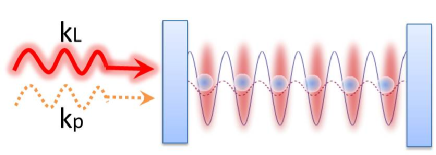
Figure 1: (Color online) Schematic diagram showing the system under consideration.

Such a model has already been realized in experiment, with the emphasis on the cavity electrodynamics stamper-kurn and cavity optomechanics stamper-kurn1 (which assumes that the atomic deviation from its equilibrium position is small). Due to the incommensurance of the trap mode and probe mode, atoms in each well of the primary lattice is subject to a different optical force induced by the probe mode. The collective effect in turn induces a Kerr-type nonlinearity (proportional to the intensity of the probe mode) to the probe-pump detuning. The strong nonlinearity thus allows for optical bistability at photon numbers below unity.

On the other hand, it is well-known that the wavefunction describing particle motion in a periodic potential with disorder can generally be grouped into extended states and localized states. The transition between them was originally studied by Anderson in the system of non-interacting electrons in a crystal with impurities anderson localization . Anderson localization describes the localization of waves in disordered media, which is considered as not only a fundamental phenomenon in condensed-matter physics but also a universal phenomenon in many areas of physics, such as light propagation in photonic crystal al in optics . The combination of ultracold atoms and optical potentials have provided a powerful playground for the study of disorder-related phenomena review article . Specifically, in the case of an optical lattice a pseudorandom potential can be generated by superimposing two standing waves of incommensurate wavelengths. The localization of atomic matter wave in such a quasiperiodic optical lattice have been experimentally observed roati08 ; deissler10 and extensively studied in theory damski03 ; modugno09 ; boers07 ; adhikari09 ; biddle10 ; roux08 ; cetoli10 ; fontanesi09 .

In the localized regime, atoms accumulate in one or several lattice sites, thus strongly deviate from its equilibrium position. Some questions then naturally arise: Whether the localization of the atomic wavefunction can be observed in the atom-cavity coupling system described above? What is the effect of cavity on localization? Will optical bistability still take place in the localized regime?

Although the study of interplay between the atomic external or internal degrees of freedom and the cavity light field have already attracted a lot of theoretical self-organization ; double well ; horak00 ; domokos02 ; moore99 ; larson08 ; meystre10 ; mekhov07 ; simons09 ; zhou09 ; pu11 ; larson11 and experimental interest cavity with bec ; esslinger09 ; esslinger08 , the new interest in this model lies in how the localization transition of the atoms gets modified inside the optical resonator. The quasi-disorder induced by the probe mode now depends on the atomic distribution, while the properties of the atomic wavefunction is intimately related to disorder. The problem is then highly nonlinear. Through this work, we expect to shed some light on the problems related to the interplay between nonlinearity and disorder.

The rest of the paper is organized as follows. Sec II introduces the theoretical model, we show that the system can be mapped into the Aubry-André model in the tight-binding limit. Sec III is devoted to the discussion of a special case, in which the physical properties of the system can be captured by a cavity-dressed asymmetric double-well system. Both the equilibrium properties and dynamics are discussed. The more general case is considered in Sec IV, in which we present numerical results and display the bistability between the atomic extended and localized states. Finally we conclude in Sec V.

II model

In order to concentrate on the nonlinearity induced by the cavity light field, we assume that the atomic s-wave scattering length is tuned to zero by means of Feshbach resonance tunable interaction . With the energy measured in units of $\hbar\omega_{R}=\hbar^{2}k_{L}^{2}/2m$ $\left(\omega_{R}\sim 2\pi\times 5\text{ kHz for }^{87}\text{Rb atoms}\right)$ and length scaled in units of $k_{L}^{-1}$, the Gross-Pitaevskii (GP) equation describing the evolution of the condensate wavefunction and the corresponding mean-field equations of motion for the cavity light field read

$$i\frac{d}{dt}\psi\left(x,t\right) =\left[-\frac{d^{2}}{dx^{2}}+U_{t}\sin^{2}\left(x\right)\right.$$

$$\left.+\left|\alpha\left(t\right)\right|^{2}U_{0}\sin^{2}\left(\beta x+\phi\right)\right]\psi\left(x,t\right),$$ (1a)

$$\frac{d}{dt}\alpha\left(t\right) =\left[i\delta_{c}-iNU_{0}\left\langle\sin^{2}\left(\beta x+\phi\right)\right\rangle-\kappa\right]\alpha\left(t\right)+\eta.$$ (1b)

Here $$\delta_{c}=\omega_{c}-\omega_{p} U_{t\left(0\right)} \phi \alpha \kappa U_{t\left(0\right)}>0 \phi=0$$ is the cavity-pump detuning, characterize the strength of atomic coupling with the trap mode and probe mode, respectively. is the phase difference between the two cavity modes. represent the amplitude for the probe mode with the decay rate . For the simplicity of the following discussion, we assume and . The bracket in Eq. (1b) is defined as

$$\langle f(x)\rangle=\int dx\,|\psi(x)|^{2}f(x)\,.$$

In the tight-binding limit, the atomic wavefunction $\psi\left(x\right)$ can be expanded over the lowest band Wannier basis $w_{j}\left(x\right)=w\left(x-j\pi\right)$ defined by the primary lattice, i.e., $\psi\left(x\right)=\sum_{j}c_{j}w_{j}\left(x\right)$ with $\sum_{j}\left|c_{j}\right|^{2}=1$. Retaining only the coupling between neighbouring Wannier states and the onsite contribution of the probe mode, after neglecting the constant terms, Eq. (1a) can be rewritten as

$$i\dot{c}_{j}=-J\left(c_{j+1}+c_{j-1}\right)-\Delta\cos\left(2\pi\beta j\right)c_{j},$$ (2)

with

$$J =-\int dx\,w_{j+1}\left(x\right)\left[-\frac{d^{2}}{dx^{2}}+U_{t}\sin^{2}\left(x\right)\right]w_{j}\left(x\right),$$

$$\Delta =\frac{\left|\alpha\right|^{2}U_{0}}{2}\int dx\cos\left(2\beta x\right)\left|w\left(x\right)\right|^{2}=\chi U_{0}\left|\alpha\right|^{2}.$$

In estimating the value of $J$ and $\Delta$, we take the Gaussian approximation for the wannier functions, which is valid for a sufficiently deep primary lattice, and from which we have

$$J =\frac{4}{\sqrt{\pi}}U_{t}^{3/4}\,\exp(-2\sqrt{U_{t}})\,,$$ (3a)

$$\Delta =\frac{\left|\alpha\right|^{2}U_{0}}{2}\,\exp(-\beta^{2}/\sqrt{U_{t}})\,.$$ (3b)

Taking the transformation

$$c_{j}=e^{ikj}\sum_{m}f_{m}e^{im\left(2\pi\beta j\right)},$$ (4)

Eq. (2) can be cast into the form

$$i\dot{f}_{m}=-\frac{\Delta}{2}\left(f_{m+1}+f_{m-1}\right)-2J\cos\left(2\pi\beta j+k\right)f_{m}.$$ (5)

Equation (5) has precisely the same form as Eq. (2) at $\Delta/J=2$, which indicates the self-duality of the Aubry-André (AA) model aa . Since Eq. (4) represents the typical discrete Fourier transform which transforms localized states into extended states and vice versa, $\Delta/J=2$ is thus regarded as the transition point between the localized states and extended states.

The linear case without atomic feedback on the cavity mode is exactly the same as those had been illustrated in modugno09 , one can observe the AA localization by increasing the value of $\Delta/J$. The AA localization resembles the Anderson localization of random systems and have been experimentally observed with a non-interacting BEC in a bichromatic optical lattice roati08 . In the following, we will investigate the nonlinear effect on AA localization brought out by the atom-cavity interaction.

III superlattice

Equation (2) indicates the periodicity $c_{j+1/\beta}=c_{j}$. In order to gain some physical insights, we first consider the special case that $1/\beta$ is an integer. Specifically, let us focus on the simple case where $1/\beta=2$. The cavity modes then form a superlattice potential (more specifically, a lattice of double-well potentials) for the condensed atoms, as shown in Fig. 2. Such a potential has been realized in the experiment nist .

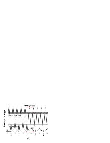
Figure 2: The superlattice potential formed by the cavity light field for $\beta=0.5$, $U_{t}=10$ and $U_{0}\left|\alpha\right|^{2}=1$. The stripes indicate the first and second Bloch bands of the primary lattice formed by the trap mode. The pertubation introduced by the probe mode is indicated by the dashed line. The label 0(1) indicates the deep (shallow) site in a supercell.

We have checked that, for the parameters considered here, the tight-binding assumption is valid and all the population are in the lowest Bloch band. Owning to the periodicity, the physics can be captured by one supercell in the region of $x\in\left[-\lambda/4,3\lambda/4\right]$, which represents a cavity-mediated double-well system for the ultracold atoms. Similar systems have also been discussed in Ref. double well . Due to the two independent cavity mode used here, the double-well potential is asymmetric, characterized by a deep well 0 and a shallow well 1.

III.1 equilibrium properties: bistability between extended and localized states

Following Eq. (2), the effective equations of motion inside one supercell can be written as

$$i\dot{c}_{0} =-2Jc_{1}-\Delta c_{0},$$

$$i\dot{c}_{1} =-2Jc_{0}+\Delta c_{1},$$ (6)

where we have used the periodic boundary condition $c_{j+2}=c_{j}$. This equation illustrates a non-interacting BEC inside a double-well potential with the tunneling coefficient $2J$ and the trap asymmetry $2\Delta$. Consider the following transformation according to Eq. (4)

$$c_{0}=f_{0}+f_{1}\text{, }c_{1}=f_{0}-f_{1},$$

the equations of motion for $f_{0}$ and $f_{1}$ reads

$$i\dot{f}_{0} =-\Delta f_{1}-2Jf_{0},$$

$$i\dot{f}_{1} =-\Delta f_{0}+2Jf_{1}.$$ (7)

Eqs. (7) has precisely the same form as Eqs. (6) with the role of $J$ and $\Delta$ interchanged, the two equations are identical at $\Delta/J=2$, which signal the critical point. The physical implication of the ciritical point can be captured via the dimensionless parameters $z=2\int_{-\pi/2}^{\pi/2}dx\left|\psi\left(x\right)\right|^{2}-1\approx\left|c_{0}\right|^{2}-\left|c_{1}\right|^{2}$, which indicate the popultion imbalance between the two wells. Under the initial condition of $c_{0}\left(0\right)=1$, $c_{1}\left(0\right)=0$ (i.e., with all atoms initially prepared in the deep well), in the linear case where $J$ and $\Delta$ are fixed external parameters, we have

$$z\left(t\right)=1-\frac{2}{1+\left(\Delta/2J\right)^{2}}\sin^{2}\sqrt{\Delta^{2}+4J^{2}}t.$$ (8)

With the increase of $\Delta/2J$ from 0 to $\infty$, Eq. (8) shows that the minimum value of $z$ increases from $-1$ to 1, indicating that the atomic wavefunction become localized and are less likely to diffuse. At the critical value of $\Delta/J=2$, the value of $z$ oscillates between 0 and 1, which means that at most half of the atoms can transport to the shallow well. In this sense we can group the atomic wavefunction into the localized state and extended state.

In the nonlinear case, we will have to take the cavity feedback into account. According to Eq. (1b)

$$\frac{d}{dt}\alpha\left(t\right)=\left[i\Delta_{c}+iNU_{0}\chi z-\kappa\right]\alpha\left(t\right)+\eta,$$ (9)

with $\Delta_{c}=\delta_{c}-NU_{0}/2$. By considering that the cavity decay rate $\kappa$ is typically much larger than the atomic oscillation frequency $J$, we adiabatically eliminate the probe field $\alpha$ from Eq. (9), replacing $\alpha$ in Eq. (3b) with

$$\alpha=\frac{\eta}{\kappa-i\left[\Delta_{c}+NU_{0}\chi z\right]}.$$ (10)

Equations (6) can be rewritten in terms of $z$ and the phase difference $\varphi$ between the amplitudes $c_{0}$ and $c_{1}$ as

$$\dot{z} =4J\sqrt{1-z^{2}}\sin\varphi,$$

$$\dot{\varphi} =-4J\frac{z}{\sqrt{1-z^{2}}}\cos\varphi+2\chi U_{0}\left|\alpha\right|^{2}.$$ (11)

The steady-state solution of the system can then be solved according to the above equations by takind the time derivative to be zero. An example is shown by the red dashed line in Fig. 3, which displays how the mean photon number of the probe mode changes with the increase of pumping amplitude $\eta/\kappa$. We can find three steady-state solutions in certain parameter region, two of them are dynamically stable while the third one is dynamically unstable, the unstable solution links the two stable ones, representing a typical dispersive optical bistability.

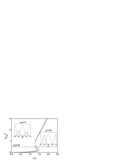
Figure 3: (Color online) The steady-state intensity of the probe mode $\left|\alpha_{ss}\right|^{2}$ versus $\eta/\kappa$ using the two-mode treatment (red-dashed line) and the self-consistent imagninary-time propagation (black dotted line). The inset show $\left|\psi\left(x\right)\right|^{2}$ (solid line) versus the optical potential (dashed line) inside one period for two different pump amplitude located at the two sides of the bistable region. The vertical black dashed line indicate the value of $\left|\alpha_{ss}\right|^{2}$ corresponding to $\Delta/J=2$. Parameters: $N=10^{4}$, $\kappa=200\omega_{R}$, $\delta_{c}=0$, $U_{0}=0.2\omega_{R}$. $U_{t}=10\omega_{R}$.

The steady-state behavior can be understood as the interplay between the double-well asymmetry and the cavity-induced nonlinearity, based on a positive feedback mechanism: With the increase of the pumping amplitude $\eta$ for the probe mode, its intensity increases as well. It results in a larger $\Delta$ and thus enhance the double-well asymmetry felt by the atoms. As a result, the atoms tend to stay in the deep well. This will give rise to a larger population imbalance $z$ and shift the cavity resonance, and will again lead to the increase of the probe mode intensity $\left|\alpha\right|^{2}$, as can be seen from Eq. (10) by setting $\Delta_{c}<-NU_{0}\chi$.

In order to understand the variation of atomic wavefunction associated with the optical bistability, we obtain the system steady-state in a self-consistent manner by propagating Eq. (1a) in imaginary-time with the steady-state value of the probe field amplitude from Eq. (1b). The numerical simulation is performed on one period $\lambda$ with periodic boundary condition. The result is displayed as the black dotted line in Fig. 3, which shows good agreement with the two-mode result. The typical wavefunctions are shown in the insets. In the linear mode without cavity feedback, as the number of the probe photon increases, the atomic system will experience a smooth crossover from the state that the atoms evenly populated between the two wells to that only populated in the deep well. Here in the cavity system, as the probe pumping rate $\eta/\kappa$ is increased, the probe photon number will show discontinuous jumps. Accompanying with this jump in photon number, the atomic wavefunction also exhibits jumps between an extended state and a localized (self-trapped) state.

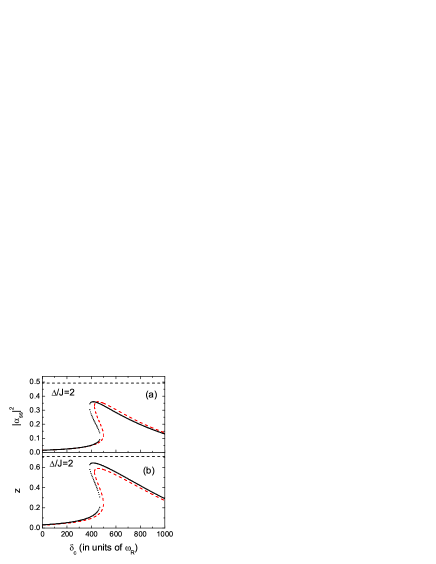
Figure 4: (Color online) (a) The steady-state intensity of the probe mode $\left|\alpha_{ss}\right|^{2}$ and (b) Inversion $z$ versus cavity-pump detuning $\delta_{c}$. The red-dashed is the result from the two-mode treatment while the black-dotted line results from the self-consistent imaginary time propagation. The parameters are the same as Fig. 3 except that $\eta=120\omega_{R}$.

We should point out here that the dispersive optical bistability is not necessarily accompanied by the transition of the atomic wavefunction across the critical point. An example is shown in Fig. 4. Here we fix the pumping amplitude $\eta$ while varying the cavity-pump detuning $\delta_{c}$, as those had been done in experiment stamper-kurn . It is clear that the region for optical bistability is located below the critical point, meaning that the bistability is taken place between extended states. We anticipate that similar situation appears in the work of Ref. stamper-kurn ; stamper-kurn1 , in which the system operates with a weak probe light field, the atomic deviation from its equilibrium position is small and thus validates the mapping into cavity optomechanics.

III.2 nonequilibrium dynamics

In order to understand how the system dynamics are modified by the nonlinear interaction, we use two different numerical methods: (i) integrate the GP equation (1a) in a self-consistent manner by assuming that the probe field amplitude adiabatically follow the the variation of the condensate wavefunction; (ii) use the two-mode model, and solve Eqs. (11) with Eq. (10). To make a comparison with the dynamics predicted in the linear case as represented by Eq. (8), we assume that the atoms are initially localized in the deep well. The numerical results are shown in Fig. 5.

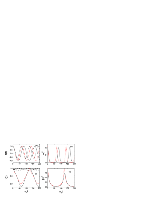
Figure 5: (Color online) Evolution of population imbalance $z$ and intensity of the probe mode $\left|\alpha\right|^{2}$ with time $t$ for $\eta/\kappa=0.5$ (upper panel) and $1.5$ (lower panel). The other parameters are the same as those in Fig. 3. The black solid line are the results calculated with numerical mithod (i) and red dashed is with method (ii). The dash dotted line is given by Eq. (8).

Figs. 5(a) and (b) are for $\eta/\kappa=0.5$, the other parameters are the same as those in Fig. 3. In this case, the probe field intensity is relatively low. As a result, the atomic dynamics show little deviation from that described by Eq. (8). However when we increase $\eta/\kappa$ to the value of $1.5$, the oscillation period of $z\left(t\right)$ experience a dramatic enhancement compared to that predicted by Eq. (8), as can be seen from Fig. 5(c). This critical slowing down takes place when the system energy approaches a critical value of that defined by an unstable saddle point, at which the contour line of energy changes its topology from a closed to an open line. This behavior is usually associated with bistability and has also been predicted in other systems before double well ; zhou09 .

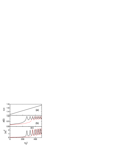
Figure 6: (Color online) The pump amplitude (a), population imbalance (b) and the probe intensity (c) versus time when the pump amplitude is swept up. The parameters are the same as those in Fig. 3. The black solid line indicate the result got with method (i) while the red dashed line use method (ii).

It is self-evident that when the system is swept across the bistable region, it cannot stay in the equilibrium solutions and non-steady state dynamics will be excited. We implement this by ramping up the pump amplitude. The population imbalance $z$ then experience a sharp transition to the localized state and exhibit periodic oscillation with most atoms stay in the deep well, as can be seen in Fig. 6(b). If $\eta$ is swept in the reverse direction, the value of $z$ can take the value of less than $0$, which means that the system has entered into the extended state, as shown in Fig. 7(b). Comparing Figs. 6 and Figs. 7, the abrupt transition exhibit a hysteretic behavior, which indicates bistability and can be readily observed in experiment.

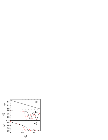
Figure 7: (Color online) Same as Fig. 6, except that the pump amplitude is swept down.

IV quasiperiodic lattice: numerical results

From the previous section we can understand that the interplay between nonlinearity and disorder may lead to bistability between atomic extended and localized states under appropriate conditions. In the more general case that $1/\beta$ is not an integer, we can only resort to numerical simulation to investigate the steady-state behavior of this system. Here we choose $\beta=\left(\sqrt{5}-1\right)/2$ as the inverse of the golden ratio. Then the cavity modes form a quasiperiodic optical lattice potential for the atoms.

Figure 8: Bistability between atomic extended and localized states. (a) intracavity photon number for the probe mode $\left|\alpha_{ss}\right|^{2}$ and (b) inverse participation ratio $P^{-1}$ plotted as function of $\eta/\kappa$. Atomic density (in log scale) and its momentum distribution for the lower bistable branch (c)(d) and upper bistable branch (e)(f) at $\eta/\kappa=1.5$. The parameters are the same as those in Fig. 3.

We focus first on the equilibrium properties of the system by numerically solve Eq. (1) with 50 lattice sites. The numerical results are shown in Fig. 8. The intracavity photon number for the probe mode as a function of the pumping rate is shown in Fig. 8(a), which exhibits hysteretic behavior typical of dispersive optical bistability. We characterize the property of atomic wavefunction with the inverse participation ratio $P^{-1}=\int dx\left|\psi\left(x\right)\right|^{4}=\sum_{j}\left|c_{j}\right|^{4}$, which is shown in Fig. 8(b). This quantity reflects the inverse of the number of the lattice sites being occupied by the atoms. Hence a larger value of $P_{-1}$ means the atoms are more localized in space. The atomic density and momentum distribution of both the upper and lower bistable branch at $\eta/\kappa=1.5$ are shown in Figs. 8(c)-(f). It is clear that in Figs. 8(c) and (d) the atomic wavefunction in the lower bistable branch display typical properties of bloch extended states with almost uniform distribution, while the associated momentum distribution $\rho\left(k\right)$ has well-defined peaks located at $k=0$, $\pm 2k_{L}$. The atomic density profile in the upper bistable branch is exponentially localized, with the corresponding momentum distribution $\rho\left(k\right)$ broadened, as can be seen in Figs. 8(e) and (f). The atomic momentum distribution in a cavity can be readily observed via absorption imaging after the time-of-flight esslinger09 . This can serve as a clear evidence that the bistability can really taken place between the atomic Bloch extended and AA localized states.

Figure 9: The pump amplitude and the probe intensity versus time when the pump amplitude is swept up (left column) and down (right column). The parameters are the same as those used in Fig. 8.

We also investigate the transition dynamics from the extended states to localized states and vice versa by ramping the pump amplitude up or down, the results are shown in Fig. 9. Similar to the dynamics displayed in Figs. 6 and 7, when the pumping strength is ramped up to exceed a critical value, or ramped down to below a lower threshold value, the system will become dynamically unstable and the probe intensity is suddenly increased or decreased, typical of dispersive optical bistability.

Figure 10: Evolution of the inverse participation ratio $P^{-1}$ when the pump amplitude is swept up (the Uppermost figure). The subsequent figure show the atomic density (in log scale) (left column) and its momentum distribution (right column). The row marked with A, B and C correspond to $\omega_{R}t=100,250$ and $350$, respectively.

The corresponding atomic dynamics are shown in Figs. 10 and 11. Fig. 10 is for the case that the pumping amplitude is ramped up. We start from an extended wavefunction, whose momentum distribution has peaks located at $k=0$, $\pm 2k_{L}$, as shown in the row marked with A. Along with the increase of the pump amplitude, the probe intensity gradually increases, the atomic spatial distribution becomes more inhomogeneous, and a small fraction of atoms will be scattered into momentum states $p=\pm 2\hbar k_{p},\pm 2\hbar\left(k_{p}-k_{L}\right),\cdot\cdot\cdot$ due to the beating of the two standing-wave cavity mode, as shown in the B row. When the pumping amplitude becomes so strong that the probe intensity greatly increases and the atomic BEC break into fragments, this is an intermediate atomic state between extended states and localized states, as shown in row C. In this process, the inverse participation ratio $P^{-1}$ finally jumped to a value around $0.05$, which is much lower than that would be expected for the present system in the localized regime (around $0.6$ as indicated in Fig. 8(b)). Comparing with the steady-state inverse participation ratio as shown in Fig. 8(b), one can see that the system can follow the instantaneous steady state (the lower branch) initially, but fails to do so after the pumping rate reaches the turning point of the lower branch. Beyond this point, the probe mode intensity jumps up and the atomic wavefunction, instead of forming a localized wavepacket as in the case of the steady state, becomes fragmented.

Figure 11: Same as Fig. 10, except that the pump amplitude is swept down. Row A, B and C correspond to $\omega_{R}t=100$, $250$ and $400$, respectively.

By contrast, when the pumping amplitude is ramped down, the inverse participation ratio $P^{-1}$ gradually decrease to a value approaching zero, as shown in Fig. 11. Contrary to Fig. 10, it displays the behavior of approximately following the instantaneous steady state adiabatically despite the occurance of bistable transition. This is because that the atoms is initially in a localized state, whose overlap with the probe mode is small, as can be seen from row A. Reducing the probe intensity only lead to the weakening of disorder, the atomic wavefunction diffuses and the sites neighbouring to the localized sites start to be macroscopically occupied, as indicated in row B and C, and the atoms becomes more and more delocalized, roughly following the steady instantaneous steady state.

V conclusion

In summary, we have investigated the system of a non-interacting BEC dispersively coupled to two standing-wave cavity modes. The equilibrium properties of the system are studied under the mean-field approximation. In the special case of $1/\beta=2$, the cavity modes form a lattice of asymmetric double-well which can be well described by a two-mode model. The results obtained from the two-mode model and the self-consistent imaginary-time propagation of the GP equation show very good agreement. Due to the interplay between the nonlinearity and disorder, bistability between the atomic extended and localized states can take place, which is associated with the occurance of optical bistability. This is also confirmed via the numerical simulation with an irrational $1/\beta$ in which case the cavity modes form a quasiperiodic lattice.

- (1) S. Gupta et al., Phys. Rev. Lett. 99, 213601 (2007).
- (2) K. W. Murch et al., Nat. Phys. 4, 561 (2008).
- (3) P. W. Anderson, Phys. Rev. 109, 1492 (1958).
- (4) T. Schwartz, G. Bartal, S. Fishman, and M. Segev, Nature 446, 52 (2006); Y. Lahini, A. Avidan, F. Pozzi, M. Sorel, R. Morandotti, D. N. Christodoulides, and Y. Silberberg, Phys. Rev. Lett. 100, 013906 (2008); I. V. Shadrivov et al., Phys. Rev. Lett. 104, 123902 (2010).
- (5) for a review, see L. Sanchez-Palencia and M. Lewenstein, Nat. Phys. 6, 87 (2010); G. Modugno, Rep. Prog. Phys. 73, 102401 (2010).
- (6) G. Roati et al., Nature 453, 895 (2008).
- (7) B. Deissler et al., Nat. Phys. 6, 354 (2010).
- (8) B. Damski, J. Zakrzewski, L. Santos, P. Zoller, and M. Lewenstein, Phys. Rev. Lett. 91, 080403 (2003).
- (9) M. Modugno, New J. Phys. 11, 033023 (2009).
- (10) D. J. Boers et al., Phys. Rev. A 75, 063404 (2007).
- (11) S. K. Adhikari and L. Salasnich, Phys. Rev. A 80, 023606 (2009); Y. Cheng and S. K. Adhikari, Phys. Rev. A 83, 023620 (2011).
- (12) G. Roux, T. Barthel, I. P. McCulloch, C. Kollath, U. Schollwöck, and T. Giamarchi, Phys. Rev. A 78, 023628 (2008).
- (13) L. Fontanesi, M. Wouters, and V. Savona, Phys. Rev. Lett. 103, 030403 (2009); Phys. Rev. A 81, 053603 (2010).
- (14) A. Cetoli and E. Lundh, Phys. Rev. A 81, 063635 (2010).
- (15) J. Biddle and S. Das Sarma, Phys. Rev. Lett. 104, 070601 (2010).
- (16) J. Sebby-Strabley, M. Anderlini, P. S. Jessen, and J. V. Porto, Phys. Rev. A 73, 033605 (2006).
- (17) P. Horak, S. M. Barnett, and H. Ritsch, Phys. Rev. A 61, 033609 (2000). P. Horak and H. Ritsch, Phys. Rev. A 63, 023603 (2001).
- (18) P. Domokos and H. Ritsch, Phys. Rev. Lett. 89, 253003 (2002); G. Szirmai and P. Domokos, Euro. Phys. J. D 48, 127 (2008).
- (19) M. G. Moore and P. Meystre, Phys. Rev. A 59, R1754 (1999); M. G. Moore, O. Zobay, and P. Meystre, Phys. Rev. A 60, 1491 (1999).
- (20) J. Larson, B. Damski, G. Morigi, and M. Lewenstein, Phys. Rev. Lett. 100, 050401 (2008); J. Larson S. Fernández-Vidal, G. Morigi, and M. Lewenstein, New J. Phys. 10, 045002 (2008).
- (21) B. Prasanna Venkatesh, J. Larson, and D. H. J. O’Dell, Phys. Rev. A 83, 063606 (2011).
- (22) R. Kanamoto and P. Meystre, Phys. Rev. Lett. 104, 063601 (2010); K. Zhang, W. Chen, M. Bhattacharya, and P. Meystre, Phys. Rev. A 81, 013802 (2010); W. Chen, K. Zhang, D. S. Goldbaum, M. Bhattacharya, and P. Meystre, Phys. Rev. A 80, 011801(R) (2009).
- (23) I. B. Mekhov, C. Maschler, and H. Ritsch, Nat. Phys. 3, 319 (2007); I. B. Mekhov, C. Maschler, H. Ritsch, Phys. Rev. Lett. 98, 100402 (2007); I. B. Mekhov and H. Ritsch, Phys. Rev. Lett. 102, 020403 (2009).
- (24) M. J. Bhaseen, M. Hohenadler, A. O. Silver, and B. D. Simons, Phys. Rev. Lett. 102, 135301 (2009); A. O. Silver, M. Hohenadler, M. J. Bhaseen, and B. D. Simons, Phys. Rev. A 81, 023617 (2010).
- (25) J. K. Asbóth, et al., Phys. Rev. A 72, 053417 (2005); D. Nagy, G. Szirmai, and P. Domokos, Eur. Phys. J. D 48, 127 (2008).
- (26) J. M. Zhang, W. M. Liu, and D. L. Zhou, Phys. Rev. A 77, 033620 (2008); 78, 043618 (2008); J. Larson and J.-P. Martikainen, Phys. Rev. A 82, 033606 (2010).
- (27) L. Zhou, H. Pu, H. Y. Ling, and W. Zhang, Phys. Rev. Lett. 103, 160403 (2009); L. Zhou, H. Pu, H. Y. Ling, K. Zhang, and W. Zhang, Phys. Rev. A 81, 063641 (2010).
- (28) Y. Dong, J. Ye, and H. Pu, Phys. Rev. A 83, 031608(R) (2011).
- (29) F. Brennecke et al., Nature 450, 268 (2007); Y. Colombe et al., Nature 450, 272 (2007).
- (30) F. Brennecke, S. Ritter, T. Donner, and T. Esslinger, Science 322, 235 (2008).
- (31) S. Ritter, et al., Appl. Phys. B 95, 213 (2009).
- (32) G. Roati et al., Phys. Rev. Lett. 99, 010403 (2007).
- (33) S. Aubry and G. André, Ann. Isr. Phys. Soc. 3, 133 (1980).