Effective tight-binding model for the iron vacancy ordered K_yFe_1.6Se₂

Abstract

We investigate the electronic structure of the ternary iron selenide K_yFe_1.6Se₂ by considering the spatial symmetry of the $\sqrt{5}\times\sqrt{5}$ vacancy ordered structure. Based on three orbitals of $t_{2g}$, which are believed to play major physics in iron-based superconductors, an effective two-dimensional tight binding Hamiltonian is constructed with the vacancy ordered structure being explicitly included. It is shown that the constructed band model, when combined with generalized Hubbard interactions, yields a spin susceptibility which exhibits both the block-checkerboard antiferromagnetism instability and the stripe antiferromagnetism instability. In particular, for large Hund’s rule couplings, the block-checkerboard antiferromagnetism wins over the stripe antiferromagnetism, in agreement with the observation in experiments. We argue that such a model with correct symmetry and Fermi surface structures should be the starting point to model K_yFe_1.6Se₂. The spin fluctuations at $\mathbf{q}$=($\pi,\pi$) suggest that interblock fluctuations of spins might play an important role in the mechanism of superconductivity occurring in this system.

I Introduction

After the discovery of superconductivity in LaFeAsO Kamihara , the finding of iron-chalcogenide superconductor $\alpha$-FeSe_x FCHsu has stimulated another intensive studies on the iron-based superconductors. Although the iron-chalcogenides and iron-pnictides have similar crystal and electronic structures, they show many differences either in superconductivity or in magnetism. For instance, the former has lower $T_{c}$ ($\sim 8K$) FCHsu  and a larger magnetic moment of the Fe ion in FeTe_1-xSe_x ($\sim 2\mu_{B}$), while the latter, e.g. La-1111, has much higher $T_{c}=26K$ Kamihara  but has a smaller magnetic moment ($\sim 0.36\mu_{B}$) for the Fe ionCruz . Even the magnetic orders are different, one is bi-collinear and the other is collinear. Recently, K, Cs or Rb intercalated FeSe superconductors A_yFe_2-xSe₂ are found. It is shown that $T_{c}$ of this system can be enhanced above $30K$ JGuo ; Maziopa ; AFWang . In this system, as the atomic ratio of Fe:Se is not 1:1, which used to be in iron-chalcogenides, iron deficiency is produced. As a result, in addition to the enhancement of $T_{c}$, a $\sqrt{5}\times\sqrt{5}$ iron vacancy ordered pattern illustrated in Fig. 1 is formed when the composition is close to K_yFe_1.6Se₂ WBao ; Bacsa ; ZWang . The vacancy ordering is followed by the magnetic transition at lower temperature $T_{N}=560K$ to the block antiferromagnetic (AFM) phase with a big moment 3.31$\mu_{B}$ WBao . Although the AFM state is observed in superconducting K_0.8Fe_1.6Se₂, evidence of nanoscale phase separation from X-ray diffraction is reported Ricci .

Previous theoretical works TAMaier ; FaWang ; YZhou ; TDas1 ; Mazin on superconductivity in the A_yFe_1.6Se₂ system were based on the band structure of KFe₂Se₂ in which the hole pocket around $\Gamma$ is absent and only electron pockets are present at M. Such Fermi surface tomography was supported by ARPES YZhang ; DMou ; TQian ; LZhao . However, since there is no experimental evidence YZhang ; TQian showing the existence of the $\sqrt{5}\times\sqrt{5}$ pattern in KFe₂Se₂, the validity of these approaches is questionable. In fact, because of the $\sqrt{5}\times\sqrt{5}$ pattern, the symmetry group changes from I4/mmm to I4/m and both the unit cell and the Brillouin zone (BZ) change as well. The underlying band structure should be very different. Indeed, the first-principles calculations of the $\sqrt{5}\times\sqrt{5}$ vacancy ordered lattice structure XWYan ; Cao indicate that a hole pocket at $\Gamma$ appears in the nonmagnetic state and as expected it loses the reflection symmetry in the x-y plane. The presence of a hole pocket at $\Gamma$ point indicates that the physics that drives superconductivity could be very different. It thus calls for a close examination based on an appropriate Hamiltonian to model the ternary iron selenide K_yFe_1.6Se₂.

In this paper, we construct a two-dimensional tight-binging model with three $t_{2g}$ orbitals for the K_0.8Fe_1.6Se₂ system with the $\sqrt{5}\times\sqrt{5}$ vacancy ordered pattern being explicitly included. Based on the general tight-binding model $H_{t}$ with symmetry imposed by the vacancy order, we fit the dispersion relation of $H_{t}$ to that of the non-magnetic state from the first-principles calculations of Ref. XWYan . Two hole pockets and two electron pockets emerges in the fitted tight-binding model. The constructed band model, when combined with generalized Hubbard interactions, yields a spin susceptibility that shows a large peak around the $\mathbf{q}$-vector ($\pi,\pi$) for the block-checkerboard AFM state. Furthermore, competition of different magnetic states is found but the block-checkerboard AFM state gets enhanced with larger Hund’s rule coupling and wins out at the end. The implication of our results to the mechanism of superconductivity is discussed. In particular, we argue that the spin fluctuations at $\mathbf{q}$=($\pi,\pi$) suggest that in analogy to spin-fluctuations in high $T_{c}$ cuprates, the interblock fluctuations of spins might play an important role in the mechanism of superconductivity occurring in this system.

II Theoretical Model

We start by considering the vacancy-ordered structure with right-handed chirality XWYan as shown in Fig. 1. In this ordered state, the unit cell includes four iron atoms (without considering Se), which we denote as $I=A$, $B$, $C$, and $D$ and three $t_{2g}$ orbitals ($d_{\overline{x}\overline{z}}$, $d_{\overline{y}\overline{z}}$, and $d_{\overline{x}\overline{y}}$) are considered in each iron. Therefore we have 12 species of electrons in a unit cell. We will suppress spin indices and denote the electron operators collectively as a vector by $\psi=\left(\psi_{1},\psi_{2},\psi_{3}\right)$ with $\psi_{\tau}=\left(d_{\tau A},d_{\tau B},d_{\tau C},d_{\tau D}\right)$, where $d_{\tau M}$ denotes the annihilation operator of electron for orbital $\tau$ at site $M$ with $\tau=1$, $2$, $3$ standing for $d_{\overline{x}\overline{z}}$, $d_{\overline{y}\overline{z}}$, $d_{\overline{x}\overline{y}}$, respectively. We will use $x$ and $y$ as the coordinates of this system and $\overline{x}\$and $\overline{y}$ as the nearest Fe-Fe directions.

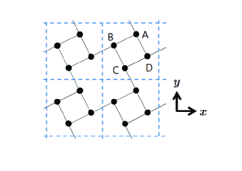
Figure 1: (Color online) The schematic representation of the $\sqrt{5}\times\sqrt{5}$ vacancy ordered lattice structure of the iron plane. The black dots denote Fe atoms and the dashed lines enclose the unit cells. $x$ and $y$ are the primitive vectors.

In previous works, the DFT band structure of the parent compound KFe₂Se₂ in which only electron pockets appear at M TAMaier ; FaWang ; YZhou ; TDas1 ; Mazin is employed. However, the parent compound KFe₂Se₂ does not have the same hopping parameters as those in the vacancy-ordered K_yFe_1.6Se₂. For example, there is no hopping between Fe atoms and vacancies. Here we shall strictly enforce the $\sqrt{5}\times\sqrt{5}$ vacancy-ordered structure and construct a tight-binding model with nearest neighbor (NN) and next-nearest neighbor (NNN) Fe-Fe hoppings, which will be classified as intra- and inter-cell ones. As the vacancy ordering appears, the reflection symmetry is lost but the four-fold-rotational symmetry is left intact. The system is invariant under 90^∘ rotations around the center of a unit cell, which is the position of Se (if the vacancy position is taken as the rotation center, the rotation has to be followed by a $P_{z}$ operation: the reflection $z\rightarrow-z$). A general hopping Hamiltonian $H_{t}$ with vacancy order being included can be written down by imposing the 90^∘ right-handed rotation symmetry: $d_{1}\rightarrow d_{2}$, $d_{2}\rightarrow-d_{1}$, $d_{3}\rightarrow-d_{3}$ accompanied with $A\rightarrow B$, $B\rightarrow C$, $C\rightarrow D$, $D\rightarrow A$. Due to its massive form, the general form of $H_{t}$ is relayed to the Appendix. After Fourier transformation, in the momentum $k$ space, it takes the form

$$H_{t}=\sum_{\mathbf{k}}\psi^{{\dagger}}(\mathbf{k})M(\mathbf{k})\psi(\mathbf{k}),$$ (1)

where $\psi(\mathbf{k})=(\psi_{1}(\mathbf{k}),\psi_{2}(\mathbf{k}),\psi_{3}(\mathbf{k}))$ with $\psi_{\tau}(\mathbf{k})=(d_{\tau A,\mathbf{k}},d_{\tau B,\mathbf{k}},d_{\tau C,\mathbf{k}},d_{\tau D,\mathbf{k}})$ and $M(\mathbf{k})$ is a $12\times 12$ matrix. Detailed characterization of all hopping parameters are tabulated in TABLE 2 and TABLE 3 in Appendix. These parameters are obtained by fitting energy dispersions (in the folded BZ) to the results of X. W. Yan et al. XWYan obtained by the generalized gradient approximation (GGA) in which the main features are four hole pockets at $\Gamma$ and four electron pockets at X in the nonmagnetic state. Our fitting gives two hole and two electron pockets, which capture basic features of this system. Fig. 2 shows our fitting results in the unfolded BZ ((a) and (c)), and in the folded BZ ((b) and (d)). In the folded BZ, there are two hole pockets around ($0,0$) and two electron pockets around ($\pi,0$); in the unfolded coordinate, one hole pocket will move to ($\pi,\pi$) and electron pockets to $\pm$($\pi/2,\pm\pi/2$).

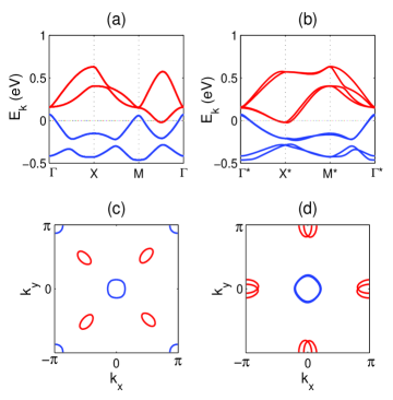
Figure 2: (Color online) The band structure of the three–orbtial model with the $\sqrt{5}\times\sqrt{5}$ lattice structure in the un-folded BZ (a) and in the folded BZ (b), and its correspoinding Fermi surfaces in (c) and (d), respectively. We have shifted the dispersion ($\mu$=0.557 in our model), such that E=0 corresponds to the Fermi level. The bands shown are only those near the Fermi level, from the eighth to the eleventh (from low energy to high energy).

	$n_{A}=n_{C}$	$n_{B}=n_{D}$	$1/4\sum_{I}n_{I}$
$n_{1}$	1.92	1.74	1.83
$n_{2}$	1.74	1.92	1.83
$n_{3}$	0.84	0.84	0.84
$\sum_{\tau}n_{\tau}$	4.50	4.50	4.50

Table 1: Particle number per Fe for different orbitals ($\tau=1,2,3$) and sites ($I=A,B,C,D$). Due to the four-fold rotation symmetry, some numbers are equal.

As for the particle number, the stoichiometric compound $A_{0.8}Fe_{1.6}Se_{2}$ gives Fe²⁺. In other words, there are six electrons for each iron. Previous three-band model works for iron-pnictides claimed four electrons per Fe in the undoped state.

In the GGA calculation XWYan , the number of electrons enclosed by Fermi surfaces is about 0.642 electrons/cell, while the number of holes enclosed by Fermi surfaces is about 0.529 holes/cell. In our model at the symmetry point, the electron number per iron is 4.5 and hence the total number of electrons is 18 per cell. The particle density for each orbital and site is listed in Table 1. As we expect, due to symmetry, $n_{1}$ at site $A$ or $C$ ($B$ or $D$) is the same as $n_{2}$ at site $B$ or $D$ ($A$ or $C$), while $n_{3}$ is uniform at every site. In addition, we found that there are about 0.52 electrons/cell and 0.52 holes/cell enclosed by Fermi surfaces. These numbers are close to those found in the GGA calculation. We note in passing that it is possible to change the chemical potential and hopping scales so that the model is away from the symmetry point and numbers of electrons/holes per cell are closer to those obtained by the GGA calculation. However, since we do not find significant changes of magnetic properties, we shall be focusing on the symmetry point.

III Magnetic and Charge Responses

Using the tight-binding model with the fitted parameters found in the last section, we can analyze linear responses of the system. We shall first calculate the generalized susceptibility in the absence of the electron-electron interaction defined by

$$\chi_{0}^{ab,cd}(\mathbf{q},i\Omega_{n}) =\int d\tau e^{i\Omega_{n}\tau}\left\langle S_{ab}^{+}(\mathbf{q},\tau)S_{cd}^{-}(-\mathbf{q},0)\right\rangle_{0}$$ (2)

$$=-\frac{1}{\beta N}\underset{\mathbf{k},i\omega_{n}}{{\textstyle\sum}}g_{ca}(\mathbf{k},i\omega_{n})g_{bd}(\mathbf{k+q},i\omega_{n}+i\Omega_{n}).$$

Here the generalized spin operators are defined by $S_{ab}^{+}\equiv\psi_{a,\uparrow}^{{\dagger}}\psi_{b,\downarrow}$ and $S_{cd}^{-}\equiv\left(S_{cd}^{+}\right)^{{\dagger}}=\psi_{d,\downarrow}^{{\dagger}}\psi_{c,\uparrow}$ with the subscript ($a,b,c,d$) being the 12 orbital indices for electrons, and the Green’s function $g_{ab}$ is given by

$$g_{ab}(\mathbf{k},i\omega_{n})=\underset{\mu}{{\textstyle\sum}}\frac{A_{a\mu}(\mathbf{k})A_{b\mu}^{\ast}(\mathbf{k})}{i\omega_{n}-E_{\mu}(\mathbf{k})},$$ (3)

where $\mu$ is the band index and $A_{a\mu}$ is the orbital-band transformation matrix, $\psi_{a}(\mathbf{k})=\underset{\mu}{{\textstyle\sum}}A_{a\mu}(\mathbf{k})\gamma_{\mu}(\mathbf{k})$. By analytic continuity, the susceptibility becomes

$$\chi_{0}^{ab,cd}(\mathbf{q},\omega) =-\frac{1}{N}\underset{\mathbf{k},\mu,\nu}{{\textstyle\sum}}A_{c\mu}(\mathbf{k})A_{a\mu}^{\ast}(\mathbf{k})A_{b\nu}(\mathbf{k+q})A_{d\nu}^{\ast}(\mathbf{k+q})$$

$$\times\frac{n_{F}\left[E_{\mu}(\mathbf{k})\right]-n_{F}\left[E_{\nu}(\mathbf{k+q})\right]}{\omega+E_{\mu}(\mathbf{k})-E_{\nu}(\mathbf{k+q})+i\delta}.$$ (4)

We now include the effect of electron-electron interaction by considering the generalized Hubbard model, in which all interactions are on the same Fe atom,

$$H_{I} =\underset{i}{{\textstyle\sum}}\underset{I=A,B,C,D}{{\textstyle\sum}}\left\{U\underset{a=1,2,3}{{\textstyle\sum}}n_{aI,i\uparrow}n_{aI,i\downarrow}\right.$$

$$+\underset{a,b(a>b)}{{\textstyle\sum}}\left[\left(U^{\prime}-\frac{J_{H}}{2}\right)n_{aI,i}n_{bI,i}-2J_{H}\mathbf{S}_{aI,i}\cdot\mathbf{S}_{bI,i}\right.$$

$$\left.\left.+J_{C}\left(d_{aI,i\uparrow}^{{\dagger}}d_{aI,i\downarrow}^{{\dagger}}d_{bI,i\downarrow}d_{bI,i\uparrow}+h.c.\right)\right]\right\}.$$ (5)

Here we simply use the same set of parameters for every site and orbital. Within this model, we calculate the random-phase approximation (RPA) susceptibilities for spin and charge

$$\chi_{s,RPA}(\mathbf{q},\omega) =\frac{\chi_{0}(\mathbf{q},\omega)}{1-\Gamma_{s}\chi_{0}(\mathbf{q},\omega)},$$ (6)

$$\chi_{c,RPA}(\mathbf{q},\omega) =\frac{\chi_{0}(\mathbf{q},\omega)}{1+\Gamma_{c}\chi_{0}(\mathbf{q},\omega)}.$$ (7)

The vertices for spin sector are $\Gamma_{s}^{\tau\tau,\tau\tau}=U$, $\Gamma_{s}^{\tau\tau^{\prime},\tau\tau^{\prime}}=U^{\prime}$, $\Gamma_{s}^{\tau\tau,\tau^{\prime}\tau^{\prime}}=J_{H}$, $\Gamma_{s}^{\tau\tau^{\prime},\tau^{\prime}\tau}=J_{C}$, and for charge sector $\Gamma_{c}^{\tau\tau,\tau\tau}=U$, $\Gamma_{c}^{\tau\tau^{\prime},\tau\tau^{\prime}}=-U^{\prime}+2J_{H}$, $\Gamma_{c}^{\tau\tau,\tau^{\prime}\tau^{\prime}}=2U^{\prime}-J_{H}$, $\Gamma_{c}^{\tau\tau^{\prime},\tau^{\prime}\tau}=J_{C}$, where nonvanishing vertices are only between the same Fe, and $\tau$ denotes orbitals and $\tau\neq\tau^{\prime}$. In the following, we shall take the relations $U^{\prime}=U-2J_{H}$ and $J_{C}=J_{H}$.

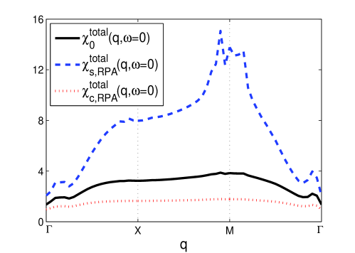
Figure 3: (Color online) Total DC susceptibilities. black solid line: bare, blue dashed line: spin, red dotted line: charge. The interaction parameters are $U=1.2eV$, $J_{H}=0.2U$, and $U^{\prime}=U-2J_{H}$.

In Fig. 3, we show the total DC susceptibilities per cell (four iron) defined by $\chi^{total}(\mathbf{q},0)={\textstyle\sum_{s,t}}\chi^{ss,tt}(\mathbf{q},0)$. Here $U$=1.2eV and $J_{H}=0.2U$ are used. The black solid line is for the bare susceptibility $\chi_{0}^{total}$, the blue dashed line is the spin susceptibility, and the red dotted line is for the charge susceptibility. As expected, electron-electron interaction strongly enhances spin susceptibility $\chi_{s}^{total}$ and induces a peak around ($\pi,\pi$). The Stoner instability for $J_{H}=0.2U$ is found to happen at $U$=1.5eV and such divergence of $\chi_{s}^{total}$ at ($\pi,\pi$) will result in the checkerboard AFM pattern as experiments observed. Therefore, the fitted tight-binding Hamiltonian explains the experimental observations. On the other hand, the charge susceptibility $\chi_{c}^{total}$ is not important here and is smaller than the bare one, which is consistent with results of Ref. Graser2009 .

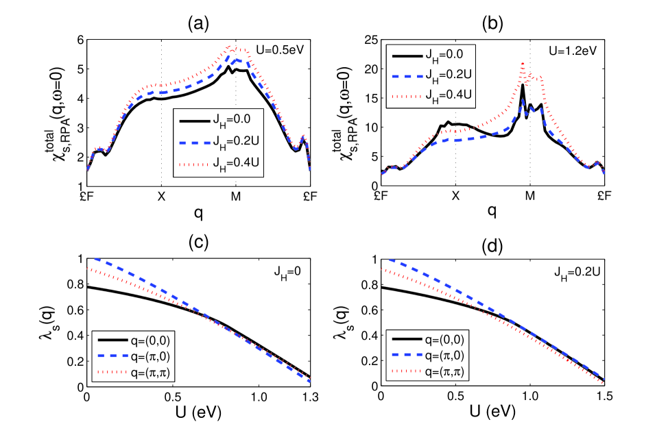
Figure 4: (Color online) Upper two panels: total spin susceptibility $\chi_{s,RPA}^{total}(\mathbf{q},0)$ at different $J_{H}$ in $U$=0.5eV (a), and in $U$=1.2eV (b). Lower two: $\lambda_{s}(\mathbf{q)}$, the minimal eigenvalue of the inverse of $\chi_{s,RPA}^{total}(\mathbf{q},0)$ at three $\mathbf{q}$ vectors in $J_{H}=0$ (c), and in $J_{H}=0.2U$ (d). The magnetic transition happens when $\lambda_{s}(\mathbf{q})=0_{+}$.

Next we investigate the effect of the Hund’s-Rule coupling. As shown in Fig. 4(a), for small $U$ (take $U$=0.5eV as a nominal example), values of $\chi_{s}^{total}$ show a monotonic behavior. However, in the large $U$ case as shown in Fig. 4(b) ($U$=1.2eV), values of $\chi_{s}^{total}$ exhibit non-monotonic behavior. In particular, the shoulder around ($\pi,0$) at large $J_{H}$ becomes a hump at $J_{H}=0$. The hump at ($\pi,0$) indicates that there is a magnetic instability for striped AFM at about $U$=1.3eV, in competition with the block-checkerboard AFM.

To further check the magnetic instability, we employ the Stoner criterion. In the multi-orbital system, the susceptibility is a matrix and magnetic instability is determined by the corresponding eigenvalues. The Stoner criterion requires one to find the first eigenvalue, $\lambda_{s}$, that reaches zero, i.e., $\lambda_{s}(\mathbf{q})=0_{+}$, where $\lambda_{s}(\mathbf{q})$ is the minimal eigenvalue of the inverse of $\chi_{s,RPA}(\mathbf{q},0)$ [$\chi_{s,RPA}^{-1}(\mathbf{q},0)=\chi_{0}^{-1}(\mathbf{q},\omega)-\Gamma_{s}$] and $\mathbf{q}$ will be the magnetic ordering vector. Fig. 4(c) and 4(d) show the behavior of $\lambda_{s}(\mathbf{q})$ versus $U$. It is seen that at $J_{H}=0$, shown in Fig. 4(c), the first eigenvalue that touches zero occurs at $\mathbf{q=}$($\pi,0$). Hence the stripe AFM is the resulting magnetic phase at $J_{H}=0$, in consistent with our previous conclusion. At larger $J_{H}$, as shown in Fig. 4(d) ($J_{H}=0.2U$), the magnetic instability occurs at $\mathbf{q=}$($\pi,\pi$). From Fig. 4(c) and 4(d), we also find that the critical value of $U$, $U_{c}$, when magnetic instability occurs, depends on $J_{H}$ as well. For $J_{H}=0$, we find that $U_{c}\sim$1.3eV, while for $J_{H}=0.2U$, we get $U_{c}\sim$1.5eV. These results all suggest that large Hund’s rule coupling stabilizes the checkerboard AFM state.

We note in passing that in the above, we do not try to distinguish whether the magnetic instability occurs exactly at ($\pi,\pi$) or not. All of these magnetic states are classified as the checkerboard AFM state. In fact, because the parameters adopted in Fig. 4 are for the system at the symmetry point, the magnetic instability does not happen exactly at ($\pi,\pi$). By changing the chemical potential, the wave vector of the magnetic instability can be shifted to be exactly at ($\pi,\pi$). This implies that the exact wave vector for the magnetic instability will generally depend on the doping level of the system.

IV Summary and discussion

In summary, in contrast to perturbative treatment of vacancies TDas2 , we have constructed an effective tight-binding model for the K_yFe_1.6Se₂ system by including exact symmetries of the Fe vacancy ordering structure. The tight-binding model includes three orbitals ($d_{\overline{x}\overline{z}}$, $d_{\overline{y}\overline{z}}$, and $d_{\overline{x}\overline{y}}$), which are considered to be the most important orbits in iron-pnictides and iron-chalcogenides. Although this system shows a large moment WBao and could be better described by including some localized moments, a proper tight-binding band structure is still required since iron-based superconductors so far are regarded as an intermediate coupling system instead of being a strong coupling system. For example, recent experimental findings from thermal transport of K_xFe_2-ySe₂ indicated it a weakly or intermediately correlated system KWang . From these aspects, it is clear that our model captured the essential low energy physics: two hole pockets around $\Gamma$ and two electron pockets around X and Y in the folded BZ. Furthermore, the constructed band model, when combined with generalized Hubbard interactions, yields a spin susceptibility which exhibits both the block-checkerboard antiferromagnetism instability and the stripe antiferromagnetism instability. In particular, for large Hund’s rule couplings, the block-checkerboard antiferromagnetism wins over the stripe antiferromagnetism, in agreement with recent observations in experiments.

While so far in this work we only consider the magnetic instability of the ternary iron selenide system, our findings also provide some insight into possible mechanism for superconductivity occurring in this system. In particular, the strong spin fluctuations at $\mathbf{q}$=($\pi,\pi$) could result in inter hole-pocket and inter electron-pocket (in opposite momenta) scatterings, which may lead to pairing with totally different symmetries of pairing. In real space, it implies that inter-block fluctuations of spins might play a similar role in analogous to spin-fluctuations in high-$T_{c}$ cuprates. While our model has not yet accounted for superconductivity observed in this system, the fitted tight-binding model shall serve as a useful starting point for developing the correct theory.

Appendix A The effective tight-binding Hamiltonian

In this appendix, we will include details for construction of the tight binding Hamiltonian. Following the symmetry argument given in the context and neglect the tetramer lattice distortion XWYan , the tight-binding Hamiltonian with NN and NNN hoppings can be written as

$$H_{t}=H_{\epsilon}+H_{12}+H_{3}+H_{12,3}.$$ (8)

Here $H_{\epsilon}$ is the on-site energy. $H_{12}$ characterizes hopping among orbitals: $d_{\overline{x}\overline{z}}$ and $d_{\overline{y}\overline{z}}$, while $H_{3}$ is the hopping term for $d_{\overline{x}\overline{y}}$ and $H_{12,3}$ describes the hopping between $d_{\overline{x}\overline{z}}$/ $d_{\overline{y}\overline{z}}$ and $d_{\overline{x}\overline{y}}$.

We shall suppress the spin index for simplicity. To consider the effect of Se atoms above and below the Fe plane periodically, the transformation $d_{3I,i}\rightarrow(-1)^{\left|i\right|}d_{3I,i}$ is included implicitly to make the hopping integrals site-independent. Due to symmetries imposed by the $\sqrt{5}\times\sqrt{5}$ vacancy ordered structure, we find that the on-site energies for $d_{\overline{x}\overline{z}}$ and $d_{\overline{y}\overline{z}}$ are different and their difference will be denoted by $\Delta$, while the on-site energy of $d_{\overline{x}\overline{y}}$ will be denoted by $\epsilon$. The on-site energy can be written as

$$H_{\epsilon}=\frac{\Delta}{2}\sum_{i}\left[d_{1A,i}^{{\dagger}}d_{1A,i}+d_{2B,i}^{{\dagger}}d_{2B,i}+d_{1C,i}^{{\dagger}}d_{1C,i}+d_{2D,i}^{{\dagger}}d_{2D,i}\right.$$

$$\left.-(1\longleftrightarrow 2)\right]$$ (9)

$$+\epsilon\sum_{i}\left[d_{3A,i}^{{\dagger}}d_{3A,i}+d_{3B,i}^{{\dagger}}d_{3B,i}+d_{3C,i}^{{\dagger}}d_{3C,i}+d_{3D,i}^{{\dagger}}d_{3D,i}\right]$$

To describe hopping terms, we will adopt the notation $t_{mn,\overline{R}}$ for intra-cell hoppings and $t_{mn,\overline{R}}^{\prime}$ for inter-cell hoppings. The subscript $mn$ are the orbital indices and $\overline{R}$ is the Fe-Fe direction. We note that because of the absence of reflection symmetry, the NN Fe-Fe hopping between $d_{\overline{x}\overline{z}}$ and $d_{\overline{y}\overline{z}}$ is allowable now. By including all possible terms allowed by symmetries, hopping terms can be generally expressed as

$$H_{12} =\sum_{i}\left\{t_{11,\overline{x}}\left(d_{1A,i}^{{\dagger}}d_{1B,i}+d_{1C,i}^{{\dagger}}d_{1D,i}+d_{2B,i}^{{\dagger}}d_{2C,i}+d_{2D,i}^{{\dagger}}d_{2A,i}\right)\right.$$ (10)

$$+t_{11,\overline{y}}\left(d_{1D,i}^{{\dagger}}d_{1A,i}+d_{1B,i}^{{\dagger}}d_{1C,i}+d_{2A,i}^{{\dagger}}d_{2B,i}+d_{2C,i}^{{\dagger}}d_{2D,i}\right)$$

$$+t_{11,\overline{x}}^{\prime}\left(d_{1B,i}^{{\dagger}}d_{1D,i-x}+d_{2A,i}^{{\dagger}}d_{2C,i+y}\right)+t_{11,\overline{y}}^{\prime}\left(d_{1A,i}^{{\dagger}}d_{1C,i+y}+d_{2B,i}^{{\dagger}}d_{2D,i-x}\right)$$

$$+t_{11,\overline{x}+\overline{y}}\left(d_{1A,i}^{{\dagger}}d_{1C,i}+d_{2B,i}^{{\dagger}}d_{2D,i}\right)+t_{11,\overline{x}-\overline{y}}\left(d_{1B,i}^{{\dagger}}d_{1D,i}+d_{2A,i}^{{\dagger}}d_{2C,i}\right)$$

$$+t_{11,\overline{x}+\overline{y}}^{\prime}\left(d_{1A,i}^{{\dagger}}d_{1D,i+y}+d_{1C,i}^{{\dagger}}d_{1B,i-y}+d_{2B,i}^{{\dagger}}d_{2A,i-x}+d_{2D,i}^{{\dagger}}d_{2C,i+x}\right)$$

$$+t_{11,\overline{x}-\overline{y}}^{\prime}\left(d_{1A,i}^{{\dagger}}d_{1B,i+x}+d_{1C,i}^{{\dagger}}d_{1D,i-x}+d_{2B,i}^{{\dagger}}d_{2C,i+y}+d_{2D,i}^{{\dagger}}d_{2A,i-y}\right)$$

$$+t_{12,\overline{x}}\left(d_{1A,i}^{{\dagger}}d_{2B,i}+d_{1C,i}^{{\dagger}}d_{2D,i}-d_{2B,i}^{{\dagger}}d_{1C,i}-d_{2D,i}^{{\dagger}}d_{1A,i}\right)$$

$$+t_{12,\overline{y}}\left(d_{2A,i}^{{\dagger}}d_{1B,i}+d_{2C,i}^{{\dagger}}d_{1D,i}-d_{1B,i}^{{\dagger}}d_{2C,i}-d_{1D,i}^{{\dagger}}d_{2A,i}\right)$$

$$+t_{12,\overline{x}}^{\prime}\left(d_{1B,i}^{{\dagger}}d_{2D,i-x}+d_{1D,i}^{{\dagger}}d_{2B,i+x}-d_{1A,i}^{{\dagger}}d_{1C,i+y}-d_{2C,i}^{{\dagger}}d_{1A,i-y}\right)$$

$$+t_{12,\overline{x}+\overline{y}}\left(d_{1A,i}^{{\dagger}}d_{2C,i}+d_{1C,i}^{{\dagger}}d_{2A,i}-d_{2B,i}^{{\dagger}}d_{1D,i}-d_{2D,i}^{{\dagger}}d_{1B,i}\right)$$

$$+t_{12,\overline{x}+\overline{y}}^{\prime}\left(d_{1A,i}^{{\dagger}}d_{2D,i+y}+d_{1C,i}^{{\dagger}}d_{2B,i-y}-d_{2B,i}^{{\dagger}}d_{1A,i-x}-d_{2D,i}^{{\dagger}}d_{1C,i+x}\right)$$

$$\left.+t_{12,\overline{x}-\overline{y}}^{\prime}\left(d_{2A,i}^{{\dagger}}d_{1D,i+y}+d_{2C,i}^{{\dagger}}d_{1B,i-y}-d_{1B,i}^{{\dagger}}d_{2A,i-x}-d_{1D,i}^{{\dagger}}d_{2C,i+x}\right)+h.c.\right\},$$

$$H_{3} =\sum_{i}\left\{t_{33,\overline{x}}\left(d_{3A,i}^{{\dagger}}d_{3B,i}+d_{3B,i}^{{\dagger}}d_{3C,i}+d_{3C,i}^{{\dagger}}d_{3D,i}+d_{3D,i}^{{\dagger}}d_{3A,i}\right)\right.$$ (11)

$$t_{33,\overline{x}}^{\prime}\left(d_{3A,i}^{{\dagger}}d_{3C,i+y}+d_{3B,i}^{{\dagger}}d_{3D,i-x}\right)+t_{33,\overline{x}+\overline{y}}\left(d_{3A,i}^{{\dagger}}d_{3C,i}+d_{3B,i}^{{\dagger}}d_{3D,i}\right)$$

$$\left.+t_{33,\overline{x}+\overline{y}}^{\prime}\left(d_{3A,i}^{{\dagger}}d_{3D,i+y}+d_{3B,i}^{{\dagger}}d_{3A,i-x}+d_{3C,i}^{{\dagger}}d_{3B,i-y}+d_{3D,i}^{{\dagger}}d_{3C,i+x}\right)+h.c.\right\},$$

$${\mathrm{a}nd}\,H_{12,3} =\sum_{i}\left\{t_{13,\overline{x}}\left(d_{3A,i}^{{\dagger}}d_{1B,i}-d_{3B,i}^{{\dagger}}d_{2C,i}-d_{3C,i}^{{\dagger}}d_{1D,i}+d_{3D,i}^{{\dagger}}d_{2A,i}\right)\right.$$ (12)

$$+t_{13,\overline{y}}\left(d_{3A,i}^{{\dagger}}d_{1D,i}-d_{3B,i}^{{\dagger}}d_{2A,i}-d_{3C,i}^{{\dagger}}d_{1B,i}+d_{3D,i}^{{\dagger}}d_{2C,i}\right)$$

$$+t_{23,\overline{x}}\left(d_{1A,i}^{{\dagger}}d_{3D,i}-d_{2B,i}^{{\dagger}}d_{3A,i}-d_{1C,i}^{{\dagger}}d_{3B,i}+d_{1D,i}^{{\dagger}}d_{3C,i}\right)$$

$$+t_{23,\overline{y}}\left(d_{1A,i}^{{\dagger}}d_{3B,i}-d_{2B,i}^{{\dagger}}d_{3C,i}-d_{1C,i}^{{\dagger}}d_{3D,i}+d_{2D,i}^{{\dagger}}d_{3A,i}\right)$$

$$+t_{13,\overline{x}}^{\prime}\left(d_{1D,i}^{{\dagger}}d_{3B,i+x}-d_{2A,i}^{{\dagger}}d_{3C,i+y}-d_{1B,i}^{{\dagger}}d_{3D,i-x}+d_{2C,i}^{{\dagger}}d_{3A,i-y}\right)$$

$$+t_{13,\overline{y}}^{\prime}\left(d_{1A,i}^{{\dagger}}d_{3C,i+y}-d_{2B,i}^{{\dagger}}d_{3D,i-x}-d_{1C,i}^{{\dagger}}d_{3A,i-y}+d_{2D,i}^{{\dagger}}d_{3B,i+x}\right)$$

$$+t_{13,\overline{x}+\overline{y}}\left(d_{1C,i}^{{\dagger}}d_{3A,i}-d_{2D,i}^{{\dagger}}d_{3B,i}-d_{1A,i}^{{\dagger}}d_{3C,i}+d_{2B,i}^{{\dagger}}d_{3D,i}\right)$$

$$+t_{13,\overline{x}-\overline{y}}\left(d_{1B,i}^{{\dagger}}d_{3D,i}-d_{2C,i}^{{\dagger}}d_{3A,i}-d_{1D,i}^{{\dagger}}d_{3B,i}+d_{2A,i}^{{\dagger}}d_{3C,i}\right)$$

$$+t_{13,\overline{x}+\overline{y}}^{\prime}\left(d_{1A,i}^{{\dagger}}d_{3D,i+y}-d_{2B,i}^{{\dagger}}d_{3A,i-x}-d_{1C,i}^{{\dagger}}d_{3B,i-y}+d_{2D,i}^{{\dagger}}d_{3C,i+x}\right)$$

$$+t_{13,\overline{x}-\overline{y}}^{\prime}\left(d_{1A,i}^{{\dagger}}d_{3B,i+x}-d_{1C,i}^{{\dagger}}d_{3D,i-x}-d_{2B,i}^{{\dagger}}d_{3C,i+y}+d_{2D,i}^{{\dagger}}d_{3A,i-y}\right)$$

$$+t_{23,\overline{x}+\overline{y}}^{\prime}\left(d_{2A,i}^{{\dagger}}d_{3D,i+y}-d_{2C,i}^{{\dagger}}d_{3B,i-y}+d_{1B,i}^{{\dagger}}d_{3A,i-x}-d_{1D,i}^{{\dagger}}d_{3C,i+x}\right)$$

$$\left.+t_{23,\overline{x}-\overline{y}}^{\prime}\left(d_{2A,i}^{{\dagger}}d_{3B,i+x}-d_{2C,i}^{{\dagger}}d_{3D,i-x}+d_{1B,i}^{{\dagger}}d_{3C,i+y}-d_{1D,i}^{{\dagger}}d_{3A,i-y}\right)+h.c.\right\}.$$

After Fourier transformation, the Hamiltonian is written in a matrix form as

$$H_{t}=\sum_{\mathbf{k}}\psi^{{\dagger}}(\mathbf{k})M(\mathbf{k})\psi(\mathbf{k})$$ (13)

where the basis vector is defined as before, $\psi(\mathbf{k})=(\psi_{1}(\mathbf{k}),\psi_{2}(\mathbf{k}),\psi_{3}(\mathbf{k}))$ with $\psi_{\tau}(\mathbf{k})=(d_{\tau A,\mathbf{k}},d_{\tau B,\mathbf{k}},d_{\tau C,\mathbf{k}},d_{\tau D,\mathbf{k}})$ and the $12\times 12$ matrix $M(\mathbf{k})$ is given by

$$M(\mathbf{k})=\left[\begin{array}[]{ccc}M_{11}(\mathbf{k})&M_{12}(\mathbf{k})&M_{13}(\mathbf{k})\\ M_{12}^{{\dagger}}(\mathbf{k})&M_{22}(\mathbf{k})&M_{23}(\mathbf{k})\\ M_{13}^{{\dagger}}(\mathbf{k})&M_{23}^{{\dagger}}(\mathbf{k})&M_{33}(\mathbf{k})\end{array}\right]$$ (14)

with elements being give by

$$M_{11}(\mathbf{k})=\left[\begin{array}[c]{cccc}\frac{\Delta}{2}&t_{11,\overline{x}}+t_{11,\overline{x}-\overline{y}}^{\prime}e^{ik_{x}}&t_{11,\overline{x}+\overline{y}}+t_{11,\overline{y}}^{\prime}e^{ik_{y}}&t_{11,\overline{y}}+t_{11,\overline{x}+\overline{y}}^{\prime}e^{ik_{y}}\\ t_{11,\overline{x}}+t_{11,\overline{x}-\overline{y}}^{\prime}e^{-ik_{x}}&-\frac{\Delta}{2}&t_{11,\overline{y}}+t_{11,\overline{x}+\overline{y}}^{\prime}e^{ik_{y}}&t_{11,\overline{x}-\overline{y}}+t_{11,\overline{x}}^{\prime}e^{-ik_{x}}\\ t_{11,\overline{x}+\overline{y}}+t_{11,\overline{y}}^{\prime}e^{-ik_{y}}&t_{11,\overline{y}}+t_{11,\overline{x}+\overline{y}}^{\prime}e^{-ik_{y}}&\frac{\Delta}{2}&t_{11,\overline{x}}+t_{11,\overline{x}-\overline{y}}^{\prime}e^{-ik_{x}}\\ t_{11,\overline{y}}+t_{11,\overline{x}+\overline{y}}^{\prime}e^{-ik_{y}}&t_{11,\overline{x}-\overline{y}}+t_{11,\overline{x}}^{\prime}e^{ik_{x}}&t_{11,\overline{x}}+t_{11,\overline{x}-\overline{y}}^{\prime}e^{ik_{x}}&-\frac{\Delta}{2}\end{array}\right],$$ (15)

$$M_{22}(\mathbf{k})=\left[\begin{array}[c]{cccc}-\frac{\Delta}{2}&t_{11,\overline{y}}+t_{11,\overline{x}+\overline{y}}^{\prime}e^{ik_{x}}&t_{11,\overline{x}-\overline{y}}+t_{11,\overline{x}}^{\prime}e^{ik_{y}}&t_{11,\overline{x}}+t_{11,\overline{x}-\overline{y}}^{\prime}e^{ik_{y}}\\ t_{11,\overline{y}}+t_{11,\overline{x}+\overline{y}}^{\prime}e^{-ik_{x}}&\frac{\Delta}{2}&t_{11,\overline{x}}+t_{11,\overline{x}-\overline{y}}^{\prime}e^{ik_{y}}&t_{11,\overline{x}+\overline{y}}+t_{11,\overline{y}}^{\prime}e^{-ik_{x}}\\ t_{11,\overline{x}-\overline{y}}+t_{11,\overline{x}}^{\prime}e^{-ik_{y}}&t_{11,\overline{x}}+t_{11,\overline{x}-\overline{y}}^{\prime}e^{-ik_{y}}&-\frac{\Delta}{2}&t_{11,\overline{y}}+t_{11,\overline{x}+\overline{y}}^{\prime}e^{-ik_{x}}\\ t_{11,\overline{x}}+t_{11,\overline{x}-\overline{y}}^{\prime}e^{-ik_{y}}&t_{11,\overline{x}+\overline{y}}+t_{11,\overline{y}}^{\prime}e^{ik_{x}}&t_{11,\overline{y}}+t_{11,\overline{x}+\overline{y}}^{\prime}e^{ik_{x}}&\frac{\Delta}{2}\end{array}\right],$$ (16)

$$M_{33}(\mathbf{k})=\left[\begin{array}[c]{cccc}\epsilon&t_{33,\overline{x}}+t_{33,\overline{x}+\overline{y}}^{\prime}e^{ik_{x}}&t_{33,\overline{x}+\overline{y}}+t_{33,\overline{x}}^{\prime}e^{ik_{y}}&t_{33,\overline{x}}+t_{33,\overline{x}+\overline{y}}^{\prime}e^{ik_{y}}\\ t_{33,\overline{x}}+t_{33,\overline{x}+\overline{y}}^{\prime}e^{-ik_{x}}&\epsilon&t_{33,\overline{x}}+t_{33,\overline{x}+\overline{y}}^{\prime}e^{ik_{y}}&t_{33,\overline{x}+\overline{y}}+t_{33,\overline{x}}^{\prime}e^{-ik_{x}}\\ t_{33,\overline{x}+\overline{y}}+t_{33,\overline{x}}^{\prime}e^{-ik_{y}}&t_{33,\overline{x}}+t_{33,\overline{x}+\overline{y}}^{\prime}e^{-ik_{y}}&\epsilon&t_{33,\overline{x}}+t_{33,\overline{x}+\overline{y}}^{\prime}e^{-ik_{x}}\\ t_{33,\overline{x}}+t_{33,\overline{x}+\overline{y}}^{\prime}e^{-ik_{y}}&t_{33,\overline{x}+\overline{y}}+t_{33,\overline{x}}^{\prime}e^{ik_{x}}&t_{33,\overline{x}}+t_{33,\overline{x}+\overline{y}}^{\prime}e^{ik_{x}}&\epsilon\end{array}\right],$$ (17)

$$M_{12}(\mathbf{k})=\left[\begin{array}[c]{cccc}0&t_{12,\overline{x}}-t_{12,\overline{x}+\overline{y}}^{\prime}e^{ik_{x}}&t_{12,\overline{x}+\overline{y}}-t_{12,\overline{x}}^{\prime}e^{ik_{y}}&-t_{12,\overline{x}}+t_{12,\overline{x}+\overline{y}}^{\prime}e^{ik_{y}}\\ t_{12,\overline{y}}-t_{12,\overline{x}-\overline{y}}^{\prime}e^{-ik_{x}}&0&-t_{12,\overline{y}}+t_{12,\overline{x}-\overline{y}}^{\prime}e^{ik_{y}}&-t_{12,\overline{x}+\overline{y}}+t_{12,\overline{x}}^{\prime}e^{-ik_{x}}\\ t_{12,\overline{x}+\overline{y}}-t_{12,\overline{x}}^{\prime}e^{-ik_{y}}&-t_{12,\overline{x}}+t_{12,\overline{x}+\overline{y}}^{\prime}e^{-ik_{y}}&0&t_{12,\overline{x}}-t_{12,\overline{x}+\overline{y}}^{\prime}e^{-ik_{x}}\\ -t_{12,\overline{y}}+t_{12,\overline{x}-\overline{y}}^{\prime}e^{-ik_{y}}&-t_{12,\overline{x}+\overline{y}}+t_{12,\overline{x}}^{\prime}e^{ik_{x}}&t_{12,\overline{y}}-t_{12,\overline{x}-\overline{y}}^{\prime}e^{ik_{x}}&0\end{array}\right],$$ (18)

$$M_{13}(\mathbf{k})=\left[\begin{array}[c]{cccc}0&t_{23,\overline{y}}+t_{13,\overline{x}-\overline{y}}^{\prime}e^{ik_{x}}&-t_{13,\overline{x}+\overline{y}}+t_{13,\overline{y}}^{\prime}e^{ik_{y}}&t_{23,\overline{x}}+t_{13,\overline{x}+\overline{y}}^{\prime}e^{ik_{y}}\\ t_{13,\overline{x}}+t_{23,\overline{x}+\overline{y}}^{\prime}e^{-ik_{x}}&0&-t_{13,\overline{y}}+t_{23,\overline{x}-\overline{y}}^{\prime}e^{ik_{y}}&t_{13,\overline{x}-\overline{y}}-t_{13,\overline{x}}^{\prime}e^{-ik_{x}}\\ t_{13,\overline{x}+\overline{y}}-t_{13,\overline{y}}^{\prime}e^{-ik_{y}}&-t_{23,\overline{x}}-t_{13,\overline{x}+\overline{y}}^{\prime}e^{-ik_{y}}&0&-t_{23,\overline{y}}-t_{13,\overline{x}-\overline{y}}^{\prime}e^{-ik_{x}}\\ t_{13,\overline{y}}-t_{23,\overline{x}-\overline{y}}^{\prime}e^{-ik_{y}}&-t_{13,\overline{x}-\overline{y}}+t_{13,\overline{x}}^{\prime}e^{ik_{x}}&-t_{13,\overline{x}}-t_{23,\overline{x}+\overline{y}}^{\prime}e^{ik_{x}}&0\end{array}\right],$$ (19)

and

$$M_{23}(\mathbf{k})=\left[\begin{array}[c]{cccc}0&-t_{13,\overline{y}}+t_{23,\overline{x}-\overline{y}}^{\prime}e^{ik_{x}}&t_{13,\overline{x}-\overline{y}}-t_{13,\overline{x}}^{\prime}e^{ik_{y}}&t_{13,\overline{x}}+t_{23,\overline{x}+\overline{y}}^{\prime}e^{ik_{y}}\\ -t_{23,\overline{x}}-t_{13,\overline{x}+\overline{y}}^{\prime}e^{-ik_{x}}&0&-t_{23,\overline{y}}-t_{13,\overline{x}-\overline{y}}^{\prime}e^{ik_{y}}&t_{13,\overline{x}+\overline{y}}-t_{13,\overline{y}}^{\prime}e^{-ik_{x}}\\ -t_{13,\overline{x}-\overline{y}}+t_{13,\overline{x}}^{\prime}e^{-ik_{y}}&-t_{13,\overline{x}}-t_{23,\overline{x}+\overline{y}}^{\prime}e^{-ik_{y}}&0&t_{13,\overline{y}}-t_{23,\overline{x}-\overline{y}}^{\prime}e^{-ik_{x}}\\ t_{23,\overline{y}}+t_{13,\overline{x}-\overline{y}}^{\prime}e^{-ik_{y}}&-t_{13,\overline{x}+\overline{y}}+t_{13,\overline{y}}^{\prime}e^{ik_{x}}&t_{23,\overline{x}}+t_{13,\overline{x}+\overline{y}}^{\prime}e^{ik_{x}}&0\end{array}\right]$$ (20)

Our fitting values are $\Delta$=0.2 and $\epsilon$=0.55, and those of the hopping integrals are listed in TABLE 2 and TABLE 3.

$t_{mn,\overline{R}}$	$\overline{R}=\overline{x}$	$\overline{R}=\overline{y}$	$\overline{R}=\overline{x}+\overline{y}$	$\overline{R}=\overline{x}-\overline{y}$
$mn=11$	-0.14	-0.09	0.03	0.03
$mn=33$	-0.05		0.3
$mn=12$	0	0	0
$mn=13$	-0.25	0	-0.05	0.15
$mn=23$	0	-0.1

Table 2: Fitted intra-cell hopping parameters between NN and NNN.

$t_{mn,\overline{R}}^{\prime}$	$\overline{R}=\overline{x}$	$\overline{R}=\overline{y}$	$\overline{R}=\overline{x}+\overline{y}$	$\overline{R}=\overline{x}-\overline{y}$
$mn=11$	-0.028	-0.04	0.024	0.024
$mn=33$	-0.05		0.35
$mn=12$	0		-0.03	-0.06
$mn=13$	-0.375	0	-0.05	0.1
$mn=23$			0.15	0.05

Table 3: Fitted inter-cell hopping parameters between NN and NNN.

References

• (1) Y. Kamihara, T. Watanabe, M. Hirano, and Hosono, J. Am. Chem. Soc. 130, 3296 (2008).
• (2) F. C. Hsu, J. Y. Luo, K. W. Yeh, T. K. Chen, T. W. Huang, P. M. Wu, Y. C. Lee, Y. L. Huang, Y. Y. Chu, D. C. Yan, and M. K. Wu, Proc. Natl. Acad. Sci. 105, 14262 (2008).
• (3) C. de la Cruz, Q. Huang, J. W. Lynn, J. Li, W. Ratcliff II, J. L. Zarestky, H. A. Mook, G. F. Chen, J. L. Luo, N. L. Wang, and P. C. Dai, Nature 453, 899 (2008).
• (4) J. Guo, S. Jin, G. Wang, S. Wang, K. Zhu, T. Zhou, M. He, and X. Chen, Phys. Rev. B 82, 180520(R) (2010).
• (5) A. Krzton-Maziopa, Z. Shermadini, E. Pomjakushina, V. Pomjakushin, M. Bendele, A. Amato, R. Khasanov, H. Luetkens, and K. Conder, J. Phys.: Condens. Matter 23, 052203 (2011).
• (6) A. F. Wang, J. J. Ying, Y. J. Yan, R. H. Liu, X. G. Luo, Z. Y. Li, X. F. Wang, M. Zhang, G. J. Ye, P. Cheng, Z. J. Xiang, and X. H. Chen, Phys. Rev. B 83, 060512(R) (2011).
• (7) W. Bao, Q. Huang, G. F. Chen, M. A. Green, D. M. Wang, J. B. He, X. Q. Wang, Y. Qiu, Chinese Phys. Lett. 28, 086104 (2011).
• (8) J. Bacsa, A. Y. Ganin, Y. Takabayashi, K. E. Christensen, K. Prassides, M. J. Rosseinsky and J. B. Claridge, Chem. Sci. 2, 1054 (2011).
• (9) Z. Wang, Y. J. Song, H. L. Shi, Z. W. Wang, Z. Chen, H. F. Tian, G. F. Chen, J. G. Guo, H. X. Yang, and J. Q. Li, Phys. Rev. B 83, 140505(R) (2011).
• (10) A. Ricci, N. Poccia, B. Joseph, G. Arrighetti, L. Barba, J. Plaisier, G. Campi, Y. Mizuguchi, H. Takeya, Y. Takano, N. Lal Saini, and A. Bianconi, Supercond. Sci. Tech. 24, 082002 (2011); A. Ricci, N. Poccia, G. Campi, B. Joseph, G. Arrighetti, L. Barba, M. Reynolds, M. Burghammer, H. Takeya, Y. Mizuguchi, Y. Takano, M. Colapietro, N. L. Saini, A. Bianconi, e-print arXiv:1107.0412.
• (11) T. A. Maier, S. Graser, P. J. Hirschfeld, and D. J. Scalapino, Phys. Rev. B 83, 100515(R) (2011).
• (12) F. Wang, F. Yang, M. Gao, Z. Y. Lu, T. Xiang, and D. H. Lee. EPL 93, 57003 (2011).
• (13) Y. Zhou, D. H. Xu, F. C. Zhang, and W. Q. Chen, EPL 95, 17003 (2011).
• (14) T. Das, and A. V. Balatsky, Phys. Rev. B 84, 014521 (2011).
• (15) I. I. Mazin, Phys. Rev. B 84, 024529 (2011).
• (16) Y. Zhang, L. X. Yang, M. Xu, Z. R. Ye, F. Chen, C. He, H. C. Xu, J. Jiang, B. P. Xie, J. J. Ying, X. F. Wang, X. H. Chen, J. P. Hu, M. Matsunami, S. Kimura, and D. L. Feng, Nature Mate. 10, 273 (2011).
• (17) D. Mou, S. Liu, X. Jia, J. He, Y. Peng, L. Zhao, L. Yu, G. Liu, S. He, X. Dong, J. Zhang, H. Wang, C. Dong, M. Fang, X. Wang, Q. Peng, Z. Wang, S. Zhang, F. Yang, Z. Xu, C. Chen, and X. J. Zhou, Phys. Rev. Lett. 106, 107001 (2011).
• (18) T. Qian, X.-P. Wang, W.-C. Jin, P. Zhang, P. Richard, G. Xu, X. Dai, Z. Fang, J.-G. Guo, X.-L. Chen, and H. Ding, Phys. Rev. Lett. 106, 187001 (2011).
• (19) L. Zhao, D. Mou, S. Liu, X. Jia, J. He, Y. Peng, L. Yu, X. Liu, G. Liu, S. He, X. Dong, J. Zhang, J. B. He, D. M. Wang, G. F. Chen, J. G. Guo, X. L. Chen, X. Wang, Q. Peng, Z. Wang, S. Zhang, F. Yang, Z. Xu, C. Chen, and X. J. Zhou, Phys. Rev. B 83, 140508(R) (2011).
• (20) X.-W. Yan, M. Gao, Z.-Y. Lu, and T. Xiang, Phys. Rev. B 83, 233205 (2011).
• (21) C. Cao and J. Dai, Phys. Rev. Lett. 107, 056401 (2011).
• (22) S. Graser, T. A. Maier, P. J. Hirschfeld, and D. J. Scalapino, New Journal of Physics 11, 025016 (2009).
• (23) T. Das, and A. V. Balatsky, e-print arXiv:1106.3289.
• (24) K. Wang, H. Lei, and C. Petrovic, Phys. Rev. B 83, 174503 (2011).