Optical Conductivity Anisotropy in the
Undoped Three-Orbital Hubbard Model for the Pnictides

Abstract

The resistivity anisotropy unveiled in the study of detwinned single crystals of the undoped 122 pnictides is here studied using the two-dimensional three-orbital Hubbard model in the mean-field approximation. Calculating the Drude weight in the $x$ and $y$ directions at zero temperature for a ${\bf Q}$=($\pi$,0) magnetically ordered state, the conductance along the antiferromagnetic direction is shown to be larger than along the ferromagnetic direction. This effect is caused by the suppression of the $d_{yz}$ orbital at the Fermi surface, but additional insight based on the momentum dependence of the transitions induced by the current operator is provided. It is shown that the effective suppression of the inter-orbital hopping $d_{xy}$ and $d_{yz}$ along the $y$ direction is the main cause of the anisotropy.

Introduction. One of the most intriguing puzzles in the study of the Fe-based high temperature superconductors johnston is the discovery of unexpected transport anisotropies in detwinned single crystals of doped and undoped AFe₂Sr₂ (A = Ba, Sr, Ca).aniso Studies of the in-plane resistivity chu showed that the effect is the largest at low doping $x$$\sim$2-4% in Ba(Fe_1-xCo_x)₂As₂, but it is present even in the undoped limit $x$=0 at low temperatures, i.e. in the magnetically ordered state with wavevector ($\pi$,0). Recent studies blomberg for the undoped 122 materials have revealed a low-temperature anisotropy (defined as $R=\rho_{b}/\rho_{a}-1$) $R$$\sim$0.4, 0.35, and 0.09, for A = Ba, Sr, and Ca, respectively. This anisotropy is counter-intuitive because along the $a$-axis the spins order in an antiferromagnetic (AFM) arrangement, while along the $b$-axis they are ferromagnetic (FM). Intuition based on, e.g., double-exchange mechanisms for manganites would suggest that the FM direction should be less resistive than the AFM one. Optical conductivity measurements concluded that this unexpected anisotropy is caused by changes in the populations of the orbitals $d_{xz}$ and $d_{yz}$ at the Fermi surface (FS),dusza in agreement with early mean-field studies where this unbalanced FS orbital population, without long-range orbital order, led to results compatible with photoemission techniques.owr

Several calculations have recently addressed the experimentally observed transport anisotropy. Using a five-orbital Hubbard model treated in a mean-field approximation, and calculating the Drude weights via the Fermi velocities at the FS, results compatible with experiments were reported. valenzuela This agreement was observed in regimes where long-range orbital order is not present, and indeed the FS redistribution of spectral weight among the $d_{xz}$ and $d_{yz}$ orbitals caused by the ($\pi$,0) magnetic orderowr is needed to understand the experimental results. Other calculations also for the five-orbital Hubbard model arrived to similar conclusions.tohyama ; valenti

In this publication, the transport anisotropy found in experiments is revisited from the perspective of a simpler three-orbital Hubbard model.three Our goal is to refine the intuitive explanations given in Refs. valenzuela, ; tohyama, , by focusing on the three orbitals widely believed to be the most important in pnictides, namely $d_{xz}$, $d_{yz}$, and $d_{xy}$, and also by identifying the electronic hopping amplitudes that cause the anisotropy. Our main results are that the experimentally observed anisotropy clearly appears in the three-orbital model, in a state that is ($\pi$,0) magnetically ordered, and it is mainly caused by the suppression of inter-hopping $d_{xz}$-$d_{yz}$ processes along the FM direction.

Models and methods. In this manuscript, the three-orbital Hubbard model for the pnictides at overall electronic density $n$=4/3 (per site and per orbital) will be used.three The hopping amplitudes that reproduce the FS in the paramagnetic state, with hole and electron pockets, were already provided and discussed in detail in Ref. three, . However, to help the readers in the understanding of our results, in Table 1 these intra- and inter-hopping amplitudes (in eV units) are provided again. From Table 1 note that the hoppings involving the $d_{xy}$ orbital, both intra-orbital and also inter-orbital with $d_{xz}$ and $d_{yz}$, are the largest in value, inducing a large Fermi velocity in the regions of the FS where the $d_{xy}$ orbital dominates. This suggests that the $d_{xy}$ may play an important role in the anisotropy. The full three-orbital Hubbard model also contains a Coulombic on-site interaction (see Eq. (11) of Ref. three, ), involving an intra-orbital Hubbard repulsion $U$, an inter-orbital repulsion $U^{\prime}$, and a Hund coupling $J$, with the constraint $U^{\prime}$=$U$-$2J$. The Hartree mean-field approximation used here has also been much discussed in previous literature and the reader is referred to Refs. three, ; rong, ; luo, for details. The mean-field order parameters are the three electronic densities of each orbital, i.e. $n_{xz}$, $n_{yz}$, and $n_{xy}$, and the three magnetic moments $m_{xz}$, $m_{yz}$, and $m_{xy}$, and they are all determined via the minimization of the Hartree mean-field energy. In the mean-field equations, the wavevector ${\bf Q}$ = ($\pi$,0) is assumed.

$t^{\alpha\beta}_{\bf{il}}$	$\bf{l}=x$	$\bf{l}=y$	$\bf{l}=x+y$	$\bf{l}=x-y$
$\alpha\beta=11$	$-0.06$	$-0.02$	$-0.03$	$-0.03$
$\alpha\beta=22$	$-0.02$	$-0.06$	$-0.03$	$-0.03$
$\alpha\beta=33$	$0.2$	$0.2$	$-0.3$	$-0.3$
$\alpha\beta=12$	$0.0$	$0.0$	$-0.01$	$0.01$
$\alpha\beta=13$	$0.2$	$0.0$	$-0.1$	$-0.1$
$\alpha\beta=23$	$0.0$	$0.2$	$-0.1$	$0.1$

Table 1: Tight-binding (TB) hopping parameters of the three-orbital Hubbard model used in this manuscript. The energy unit is eV. The labeling convention is $1$=$d_{xz}$, $2$=$d_{yz}$, $3$=$d_{xy}$. The 13 and 23 hoppings are all affected by a factor $(-1)^{|i|}=(-1)^{{i_{x}}+{i_{y}}}$, with ${\bf i}$=($i_{x}$,$i_{y}$) being the label of the Fe sites of a two-dimensional lattice. This modulation takes into account the two-Fe unit cell of the original FeAs layers.three The TB Hamiltonian is defined as $H_{\rm HT}$=$\sum_{{\bf i}{\bf l}\alpha\beta\sigma}t^{\alpha\beta}_{{\bf i}{\bf l}}(c^{\dagger}_{{\bf{i}},\alpha,\sigma}c_{{\bf{i+l}},\beta,\sigma}+h.c.)$, where $c^{\dagger}_{{\bf{i}},\alpha,\sigma}$ creates an electron at orbital $\alpha$ of site ${\bf i}$ with spin projection $\sigma$. ${\bf i+l}$ denotes nearest and next-nearest neighbor sites to ${\bf i}$.

Let us focus now on the optical conductivity $\sigma(\omega)$. Following well-known computational studies of $\sigma(\omega)$ in the context of the cuprates,Elbio let us define first the paramagnetic current operators in the two directions as

$$\begin{split}{\hat{j}}_{x}&=\sum_{\langle\mathbf{i,l=\hat{x},\hat{x}+\hat{y},\hat{x}-\hat{y}}\rangle}\sum_{\alpha,\beta,\sigma}-it^{\alpha\beta}_{\mathbf{il}}(c^{\dagger}_{\mathbf{i},\alpha,\sigma}c_{\mathbf{i+l},\beta,\sigma}-h.c.),\\ {\hat{j}}_{y}&=\sum_{\langle\mathbf{i,l=\hat{y},\hat{x}+\hat{y},-\hat{x}+\hat{y}}\rangle}\sum_{\alpha,\beta,\sigma}-it^{\alpha\beta}_{\mathbf{il}}(c^{\dagger}_{\mathbf{i},\alpha,\sigma}c_{\mathbf{i+l},\beta,\sigma}-h.c.),\\ \end{split}$$ (1)

while the kinetic energy operators are

$$\begin{split}{\hat{T}}_{x}&=\sum_{\langle\mathbf{i,l=\hat{x},\hat{x}+\hat{y},\hat{x}-\hat{y}}\rangle}\sum_{\alpha,\beta,\sigma}t^{\alpha\beta}_{\mathbf{il}}(c^{\dagger}_{\mathbf{i},\alpha,\sigma}c_{\mathbf{i+l},\beta,\sigma}+h.c.),\\ {\hat{T}}_{y}&=\sum_{\langle\mathbf{i,l=\hat{y},\hat{x}+\hat{y},-\hat{x}+\hat{y}}\rangle}\sum_{\alpha,\beta,\sigma}t^{\alpha\beta}_{\mathbf{il}}(c^{\dagger}_{\mathbf{i},\alpha,\sigma}c_{\mathbf{i+l},\beta,\sigma}+h.c.).\\ \end{split}$$ (2)

The total current, up to the first order term in the external field ${\bf{A}}$=($A_{x}$,$A_{y}$), can be written as ${\hat{J}}_{x}$=$({\hat{j}}_{x}+{\hat{T}}_{x}A_{x})/N$ and ${\hat{J}}_{y}$=$({\hat{j}}_{y}+{\hat{T}}_{y}A_{y})/N$. The real part of the optical conductivity in the $x$ direction is given by: Elbio

$$\begin{split}Re\sigma_{xx}(\omega)&=D_{x}\delta(\omega)\\ &+\frac{\pi}{N}\sum_{n\not=0}\frac{|\langle\phi_{0}|{\hat{j}}_{x}|\phi_{n}\rangle|^{2}}{E_{n}-E_{0}}\delta(\omega-(E_{n}-E_{0})),\\ \end{split}$$ (3)

and from the $\sigma(\omega)$ sum-rule, it can be shown that the Drude weight in the $x$ direction $D_{x}$ is Elbio

$$\begin{split}\frac{D_{x}}{2\pi}&=\frac{\langle\phi_{0}|-{\hat{T}}_{x}|\phi_{0}\rangle}{2N}-\frac{1}{N}\sum_{n\not=0}\frac{|\langle\phi_{0}|{\hat{j}}_{x}|\phi_{n}\rangle|^{2}}{E_{n}-E_{0}},\\ \end{split}$$ (4)

where $\phi_{0}$ is the many-body ground state (in this case the mean-field ${\bf Q}$=($\pi$,0) state), and $\phi_{n}$ represents the many-body excited states, also produced in the mean-field calculation, with $E_{0}$ and $E_{n}$ their corresponding energies. The optical conductivity and Drude weight in the $y$ direction can be obtained and expressed similarly. $N$ is the number of sites. In our calculation, the Dirac $\delta$ functions are regularized as a Lorentzian $\delta(\omega)$$\approx$$(1/\pi)\epsilon/(\omega^{2}+\epsilon^{2})$ with a small but finite broadening parameter $\epsilon$.

Results. One of the main results found in our study is shown in Fig. 1 where $\sigma(\omega)$ in the two directions is shown for a state with magnetic order ($\pi$,0). The values of the couplings $U$ and $J$ are representative of the so-called “physical region” that was previously unveiled for the same three-orbital model.luo In other words, by a comparison between neutron scattering and photoemission experiments against mean-field results, in previous studies it was concluded that the three-orbital model has a “physical region” (where theory matches experiments) in the range $U$$\sim$[0.7,1.3] and $J/U$$\sim$[0.15,0.33],luo where the state is simultaneously magnetic and metallic as in pnictide parent compounds. Our $\sigma(\omega)$ study is restricted to that “physical region”.

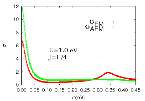
Figure 1: (color online) Example showing $\sigma(\omega)$ in the “physical region”luo of the three-orbital model ($\epsilon$=0.02). The unit of $\sigma(\omega)$ is $e^{2}/\hbar$. The couplings are $U=1.0$ eV and $J$=$U/4$. The AFM direction (i.e. the $x$ direction for magnetic wavevector $(\pi,0)$) has a larger zero frequency conductivity than the FM direction, as in experiments. The FM direction also has a peak at a finite frequency $\sim$$J$.

Figure 1 shows that $\sigma(\omega)$ for the three-orbital model is found to be in good qualitative agreement with experiments, namely at small frequency $\omega$, where the Drude peak is located, the weight of this peak is larger along the AFM direction (the $x$ direction) than along the FM direction. Similar results were obtained in the entire “physical region”, see Fig. 2. In addition, the finite frequency peak in the FM direction was found to scale with $J$. The ratio $D_{\rm AFM}$/$D_{\rm FM}$ (i.e. $D_{x}$/$D_{y}$) in the range of $U$ shown in Fig. 2 varies approximately between 1.6 and 2.2, in qualitative agreement with results for the five-orbital model.valenzuela ; tohyama Thus, it is here concluded that the three-orbital model three is sufficient to reproduce the d.c. conductivity anisotropy found in experiments. aniso

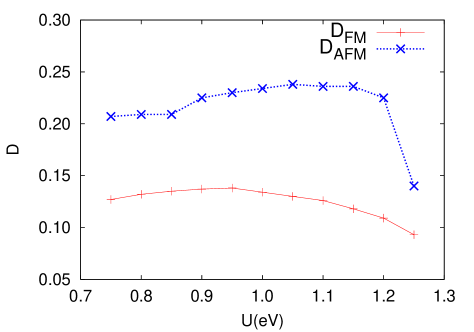
Figure 2: (color online) Drude weight/$\pi$ $vs.$ $U$ in the “physical region” of the three-orbital model, at $J$=$U/4$. In this regime, the inequality $D_{\rm AFM}$$>$$D_{\rm FM}$ holds. As $U$ increases toward the upper limit shown, the Drude weights in both directions are reduced due to increasing insulating tendencies.luo

For completeness, in Fig. 3(a) the population of the three orbitals is shown in the range of $U$’s studied. From this figure, it is clear that there is no orbital order since the orbitals $d_{xz}$ and $d_{yz}$ are nearly identically populated. Further increasing $U$ eventually leads to a regime of orbital-order,three but the opening of a gap renders the system insulating. It is important to note that Fig. 3(a) contains results obtained by integrating the orbital-selective density-of-states over all frequencies, while if the focus is only the vicinity of the FS, the orbital-weight redistribution phenomenon is observed.three As shown below, this redistribution is important to understand the anisotropy.

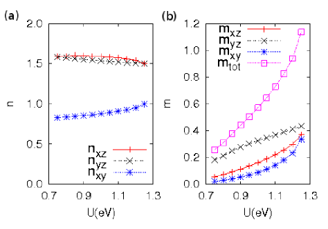
Figure 3: (color online) (a) Charge density of each orbital $vs.$ $U$ in the “physical region” of the three-orbital model, at $J$=$U/4$, and for spin order $(\pi,0)$. (b) $m_{\alpha}$ $vs.$ $U$ in the same $U$ range, at $J$=$U/4$, and for spin order $(\pi,0)$.

In addition, Fig. 3(b) shows that the magnetic moment in the range investigated is compatible with pnictides neutron experiments, ranging from $\sim$0.25 Bohr magnetons ($\mu_{B}$) for the 1111 to $\sim$1 $\mu_{B}$ for the 122 compounds.luo

Intuitive origin of the anisotropy. While the notion of an orbital weight redistribution at the FS is well established,owr ; valenzuela with the $d_{yz}$ orbital suppressed for ${\bf Q}$=($\pi$,0), it is desirable to develop a more intuitive understanding of its influence on transport properties. For this purpose, the kinetic energy and current operators will be expressed in momentum space as:

$$\begin{split}{\hat{T}_{a}}&=\sum_{\bf{k}}\sum_{\alpha,\beta,\sigma}t_{a}^{\alpha\beta}({\bf{k}})c^{\dagger}_{{\bf{k}},\alpha,\sigma}c_{{\bf{k}},\beta,\sigma}=\sum_{\bf{k}}{\hat{T}_{a}}({\bf{k}}),\\ {\hat{j}_{a}}&=\sum_{\bf{k}}\sum_{\alpha,\beta,\sigma}j_{a}^{\alpha\beta}({\bf{k}})c^{\dagger}_{{\bf{k}},\alpha,\sigma}c_{{\bf{k}},\beta,\sigma}=\sum_{\bf{k}}{\hat{j}_{a}}({\bf{k}}),\\ \end{split}$$ (5)

where $a$ is the direction index ($x$, $y$). From Eq.(4), the ${\bf k}$ contribution (unfolded first Brillouin zone) to the Drude weight is defined as $D_{a}({\bf{k}})$=$D_{1,a}({\bf{k}})$-$D_{2,a}({\bf{k}})$, where

$$\begin{split}\frac{D_{1,a}({\bf{k}})}{2\pi}&=\frac{\langle\phi_{0}|-{\hat{T}_{a}}({\bf{k}})|\phi_{0}\rangle}{2N},\\ \frac{D_{2,a}({\bf{k}})}{2\pi}&=\frac{1}{N}\sum_{n\not=0}Re\frac{\langle\phi_{0}|{\hat{j}_{a}}({\bf{k}})|\phi_{n}\rangle\times\langle\phi_{n}|{\hat{j}_{a}}|\phi_{0}\rangle}{E_{n}-E_{0}},\\ \end{split}$$ (6)

since summing over $\bf{k}$ leads to Eq. (4).

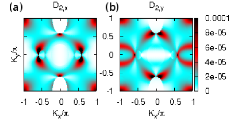
Figure 4: (color online) $D_{2,a}(\bf{k})/\pi$ in the “physical region”luo of the three-orbital model ($U$=$1.0$ eV, $J$=$U/4$) and with spin order $(\pi,0)$. For a discussion of the results see text.

From Fig. 4(b) it is clear that the $(\pi,0)$ pocket contributes significantly to $D_{2,y}$ since this wavevector region has sizable intensity. However, the contribution of the $(0,\pi)$ pocket to $D_{2,x}$ is negligible, thus inducing the significant anisotropy observed in the overall Drude weight (note that the rest of the highly intense features in $D_{2,y}$ are $\pi$/2-rotated those of $D_{2,x}$ and thus do not contribute to the anisotropy). The reason is the orbital weight redistribution at the FS: according to nesting scenarios, the $(0,0)$ pocket (with mainly $d_{xz}$ and $d_{yz}$ character), interacts with the $(\pi,0)$ pocket (mainly $d_{xy}$ and $d_{yz}$) when the magnetic wavevector is $\bf{Q}$=($\pi$,0). This interaction needs to be intra-orbital,recent hence the $d_{yz}$ states at the $(\pi,0)$ pocket are raised above the FS, while the $d_{xy}$ states are not. On the other hand, the $(0,\pi)$ states are not moved above the FS if ${\bf Q}$=($\pi$,0), and hence this phenomenon does not occur for $D_{2,x}$. Note that the results of Fig. 4 based on the Drude weights directly address the anisotropy in transport, and complements the analysis based on the orbital-weight redistribution.owr ; valenzuela Also note that a similar analysis of $D_{1,y}$ and $D_{1,x}$ (not shown) does not lead to the same clear anisotropy that $D_{2,a}$ provides.

To further simplify the understanding of the anisotropy evident in Fig. 4 let us now focus on the most relevant electronic hopping processes. Analyzing the values of the hopping amplitudes (Table 1), it is clear that those involving the $d_{xy}$ orbital (both inter- and intra-orbital) should be the most relevant since the other hoppings are much smaller in magnitude. The direct intra-orbital hopping $d_{xy}$-$d_{xy}$ ($t^{33}_{\bf{il}}$ in Table 1) is not suppressed at the FS and should equally contribute to charge transport in both directions. Thus, the conductance should not drop to zero in any of the two directions due to this intra-orbital contribution. However, the inter-orbital hopping $d_{xy}$-$d_{yz}$ is suppressed at the FS in a magnetic state ($\pi$,0). This hopping occurs only along the $y$ direction, as previously discussed.three On the other hand, the hopping $d_{xy}$-$d_{xz}$ is not suppressed and can contribute to electronic hopping along the $x$ direction. For these reasons, an asymmetry is expected between the $x$ and $y$ directions in transport, as found in Fig. 1. In addition, for $\bf{k}$ close to the $(\pi,0)$ pocket the inter-orbital $d_{xy}$-$d_{yz}$ hopping, which only exists along the $y$ direction, needs an excitation to contribute to $\sigma(\omega)$ along the FM direction ($y$-axis) because $d_{yz}$ is suppressed at the FS. This observation justifies the presence of a peak scaling with $J$ in $\sigma_{\rm FM}$ (Fig. 1).

To transform the intuition developed above based on hopping amplitudes into actual transport properties, the Drude weight will also be decomposed according to the hoppings corresponding to the different orbitals, via the following definitions:

$$\begin{split}\frac{D_{a}^{\alpha\beta}}{2\pi}&=\frac{\langle\phi_{0}|-{\hat{T}}_{a}^{\alpha\beta}-{\hat{T}}_{a}^{\beta\alpha}|\phi_{0}\rangle}{2N}\\ &-\frac{1}{N}\sum_{n\not=0}Re\frac{\langle\phi_{0}|{\hat{j}}_{a}^{\alpha\beta}+{\hat{j}}_{a}^{\beta\alpha}|\phi_{n}\rangle\langle\phi_{n}|{\hat{j}_{a}}|\phi_{0}\rangle}{E_{n}-E_{0}},\\ \end{split}$$ (7)

for inter-orbital hopping ($\alpha$$\neq$$\beta$) ($a$=$x$,$y$). The operators in Eq. (7) arise from Eq. (2) via ${\hat{T}}_{a}$=$\sum_{a,\alpha\beta}{\hat{T}}_{a}^{\alpha\beta}$ and ${\hat{j}}_{a}$=$\sum_{a,\alpha\beta}{\hat{j}}_{a}^{\alpha\beta}$. For the case of intra-orbital, the diagonal Drude weight $D_{a}^{\alpha\alpha}$ is obtained from Eq. (7) by replacing ${\hat{T}}_{a}^{\alpha\beta}$+${\hat{T}}_{a}^{\beta\alpha}$ by ${\hat{T}}_{a}^{\alpha\alpha}$ and ${\hat{j}}_{a}^{\alpha\beta}$+${\hat{j}}_{a}^{\beta\alpha}$ by ${\hat{j}}_{a}^{\alpha\alpha}$. The several Drude components obtained by this procedure are in Table 2. From this Table, it can be seen that the main anisotropy arises from the fact that $D_{x}^{13}$$\sim$0.125 is an order of magnitude larger than $D_{y}^{23}$$\sim$0.011, due to the FS suppression of the $d_{yz}$ orbital. The rest of the contributions in Table 2 that are unrelated to the inter-orbital hopping involving $d_{xy}$ are similar in both directions and are not relevant to understand the anisotropy. Actually, for the largest of those, the naive intuition suggesting a better conductance along the FM direction is satisfied since $D_{y}^{33}$$>$$D_{x}^{33}$.

Summary. A mean-field study of $\sigma(\omega)$ employing a three-orbital Hubbard model for the magnetically ordered parent compounds of the pnictides has been here reported. In agreement with experiments, the conductance along the AFM direction is shown to be larger than along the FM direction. The simplicity of this model allowed us to reduce this effect to an intuitive picture: (i) The AFM conductance behaves normally with a notorious suppression of its value as compared with the non-interacting limit due to spin scattering, in agreement with intuition. (ii) However, along the FM direction the drastic reduction in the weight of the $d_{yz}$ orbital at the FS leads to a large effective suppression of the $d_{xy}$-$d_{yz}$ hopping and associated conductance along that FM direction, causing the anisotropy found experimentally.

$\alpha\beta$	$11$	$22$	$33$	$12$	$13$	$23$
$D_{x}^{\alpha\beta}$	$0.019$	$-0.003$	$0.073$	$0.013$	$0.125$	$0.005$
$D_{y}^{\alpha\beta}$	$0.020$	$0.002$	$0.087$	$0.014$	$-0.01$	$0.011$

Table 2: Drude weight$/\pi$ decomposed into the different orbitals ($1$=$d_{xz}$, $2$=$d_{yz}$, $3$=$d_{xy}$) of the three-orbital model working at $U$=$1.0$ eV and $J$=$0.25U$. Finding negative Drude weights in some cases is a well-known effectElbio arising from differences of two large numbers in Eq. (4).

Acknowledgments. Work supported by the U.S. Department of Energy, Office of Basic Energy Sciences, Materials Sciences and Engineering Division.

References

- (1) D. C. Johnston, Adv. Phys. 59, 803 (2010).
- (2) For a recent review see I. R. Fisher, L. Degiorgi, and Z. X. Shen, arXiv:1106.1675.
- (3) J-H. Chu et al., Science 329, 824 (2010).
- (4) E. C. Blomberg at al., Phys. Rev. B 83, 134505 (2011); and references therein.
- (5) A. Dusza et al., arXiv:1107.0670.
- (6) M. Daghofer et al., Phys. Rev. B 81, 180514(R) (2010).
- (7) B. Valenzuela, E. Bascones, and M. J. Calderón, Phys. Rev. Lett. 105, 207202 (2010).
- (8) K. Sugimoto, E. Kaneshita, and T. Tohyama, J. Phys. Soc. Jpn. 80, 033706 (2011).
- (9) Density functional results are also compatible with experiments (J. Ferber et al., Phys. Rev. B 82, 165102 (2010)).
- (10) Maria Daghofer et al., Phys. Rev. B 81, 014511 (2010).
- (11) Qinlong Luo et al., Phys. Rev. B 82, 104508 (2010).
- (12) Rong Yu et al., Phys. Rev. B 79, 104510 (2009).
- (13) E. Dagotto., Rev. Mod. Phys 66, 763 (1994).
- (14) A. Nicholson et al., arXiv: 1107.2962.
- (15) For the case of doped systems other effects, such as charge stripes (Qinlong Luo et al., Phys. Rev. B 83, 174513 (2011)), may be needed to quantitatively understand the transport anisotropy which is larger than for the undoped case.