Towards precise ages for single stars in the field.
Gyrochronology constraints at several Gyr using wide binaries.
I. Ages for initial sample

Abstract

We present a program designed to obtain age-rotation measurements of solar-type dwarfs to be used in the calibration of gyrochronology relations at ages of several Gyr. This is a region of parameter space crucial for the large-scale study of the Milky Way, and where the only constraint available today is that provided by the Sun. Our program takes advantage of a set of wide binaries selected so that one component is an evolved star and the other is a main-sequence star of FGK type. In this way, we obtain the age of the system from the evolved star, while the rotational properties of the main sequence component provides the information relevant for gyrochronology regarding the spin-down of solar-type stars. By mining currently available catalogs of wide binaries, we assemble a sample of 37 pairs well positioned for our purposes: 19 with turnoff or subgiant primaries, and 18 with white dwarf components. Using high-resolution optical spectroscopy, we measure precise stellar parameters for a subset of 15 of the pairs with turnoff/subgiant components, and use these to derive isochronal ages for the corresponding systems. Ages for 16 of the 18 pairs with white dwarf components are taken from the literature. The ages of this initial sample of 31 wide binaries range from 1 to 9 Gyr, with precisions better than $\sim 20$% for almost half of these systems. When combined with measurements of the rotation period of their main sequence components, these wide binary systems would potentially provide a similar number of points useful for the calibration of gyrochronology relations at very old ages.

1 Introduction

Understanding the detailed formation and evolution of systems such as star clusters and galaxies requires knowledge of the ages of their constituent stars with sufficient precision. The derived star formation histories of the populations of stars in all types of galaxies provide crucial constraints on models of the formation of structure on cosmological scales (Springel & Hernquist, 2003; Nagamine et al., 2005; Conroy & Wechsler, 2009). In the context of our own Milky Way, for example, the various theoretical models for the formation and evolution of the disk of the Galaxy make different predictions for the age distributions of thin- and thick-disk stars (Abadi et al., 2003; Brook et al., 2007; Schönrich & Binney, 2009). Even though large amounts of information on the chemistry and kinematics of these objects are and will continue to become available, without a proper knowledge of the ages of thin- and thick-disk members it will not be possible to determine which are the more realistic scenarios. Similarly, age-dating of the numerous stellar streams being discovered by modern surveys would help trace back their origin and therefore contribute to a better understanding of the recent accretion history of the Galaxy. Exoplanet research could also benefit from precise determinations of stellar ages since the ages of host stars can be used as constrains for dynamical models of planetary systems and migration. Moreover, the ages of host stars would be crucial for investigations of biological evolution in potentially habitable planets (Soderblom, 2010).

Unfortunately, the determination of stellar ages is possible only in a few cases, typically for sets of stars that can be safely assumed to be more or less coeval (e.g., clusters, associations, etc.) and for very nearby stars for which a wealth of accurate information such as distances, luminosities, and detailed chemical compositions are also available. For plain and simple isolated stars in the Galactic field just outside the very immediate solar neighborhood, reliable ages are simply not possible yet. This lack of knowledge of the age distribution of stars in the Milky Way thus constitutes a severe limitation under the perspective of cosmology and galaxy formation, as it prevents an adequate investigation of the details of the formation history of our Galaxy. Upcoming experiments such as Gaia and LSST aim to change this situation by measuring the properties of many millions of stars with very high accuracy but, as of today, stellar ages will still need to be derived from isochrone fitting. While historically this has been the most successful method for deriving stellar ages in many branches of astronomy, it suffers from limitations that become particularly restrictive when dealing with the needs of a more ambitious mapping of the star formation histories of the components of the Milky Way. In this context, some of the limitations of isochronal ages include their high sensitivity to errors in distance (Soderblom et al., 2005) and stellar parameters, systematic biases arising from the sampling of isochrone points (Pont & Eyer, 2004; Nordstrom et al., 2004; Jørgensen & Lindegren, 2005; da Silva et al., 2006), the impact of poorly understood stellar evolutionary processes such as microscopic diffusion, convective overshoot, gravitational settling, and others (VandenBerg et al., 2002; Demarque et al., 2004; Michaud et al., 2010), and the unavoidable fact that the method is most sensitive to evolved, thus relatively massive, stars, and not so much to stars on the main sequence (MS). Thus the importance of seriously exploring any alternative to the use of stellar models for deriving ages of field stars.

One of such alternatives is that offered by gyrochronology (Skumanich, 1972; Barnes, 2003, 2007). The method takes advantage of the fact that MS stars of FGK-types are known to lose angular momentum in a predictable way, as seen by the measured surface rotation rates of stars in a sequence of clusters of different ages (Stauffer et al., 1987; Radick et al., 1995; Irwin et al., 2006; Messina et al., 2008; Meibom et al., 2009; Collier Cameron et al., 2009; Hartman et al., 2009, 2010; Delorme et al., 2011; Meibom et al., 2011a). Thus, if it were possible to map and quantitatively calibrate with precision such spin down from very young to very old ages, it should in principle be possible to apply those gyrochronology relations to single stars in the field and, by measuring their surface rotation rates and colors (a proxy for their masses), readily obtain their ages.

While there exists a growing body of observational evidence in support of the possibility of gyrochronology, a solid theoretical understanding still needs to be fully developed. The physics at the heart of the method involves the self-regulated interaction between stellar phenomena that are not easily modeled, such as differential internal rotation, magnetic fields interior to stars, and magnetized stellar winds that are able to carry angular momentum away. For a discussion of these processes and their interaction in the context of a theoretical framework for gyrochronology, see Barnes (2003, 2010). In the present paper, we approach the subject from the perspective of the empirical calibration of gyrochronology relations for use as a tool for the age dating of field stars.

Until very recently, reliably calibrated gyrochronology relations existed only for stars younger than about 0.5 Gyr, for the simple reason that such age corresponded to the oldest clusters for which rotation periods had been measured for a large enough number of member stars. The only constraint beyond this point corresponded to the Sun, thus preventing a good calibration of gyrochronology relations for stars a few Gyr old. Although there was never a lack of older clusters to extend these relations to correspondingly older ages, the limitation was of a technical nature as older stars become progressively less active, thus complicating the task of measuring the already small photometric modulation due to starspots coming into and out of the line-of-sight as the stars rotate.

The above situation started to improve recently when Meibom et al. (2011b) published rotation periods for stars in the 1 Gyr old cluster NGC 6811. Theirs is a comprehensive program that takes advantage of the existence of three open clusters within the field of view of NASA’s Kepler mission, and thus it is expected that their work for NGC 6811 will be repeated for the cases of NGC 6819 and NGC 6791, which would provide calibrations of gyrochronology relations at 2.5 and, possibly, 9 Gyr of age, respectively.

In this paper we introduce an ongoing program devised to place constraints for gyrochronology relations in the regime of ages where the large majority of field stars fall, i.e., from one to several Gyr. We achieve this by studying samples of wide stellar binaries chosen so that one of their components is an evolved star (either turnoff, subgiant, or white dwarf), while their secondaries are regular MS stars of FGK types. Therefore, with the evolved primary potentially well suited to provide a reliable age for the system, a measurement of the rotation period of the MS secondary automatically provides a point useful for the calibration of gyrochronology relations at the corresponding age.

The availability of large numbers of wide binaries with the above characteristics, both from existing as well as upcoming all-sky surveys and catalogs, suggests that these objects could in principle provide quite a large and varied pool of gyrochronology constraints. Indeed, being a representative sample of the mix of stellar populations that surround the solar neighborhood, wide binaries span a large range of stellar properties, including age, mass, and metallicity. For these reasons, a gyrochronology program based on these objects has the potential of populating the phase space of relevant variables (i.e., age, mass, and rotation period) more densely and continuously than it may be possible with only star cluster observations.

The first step in our program, therefore, involves the determination of stellar ages for a sample of wide binary components suitable of being dated. Today, precise stellar ages for individual stars can be readily computed for stars that either (a) began relatively recently to evolve away from the MS, such as turnoff stars and subgiants, or (b) did this a long time ago and are now in the white dwarf (WD) phase of their evolution. For recently evolved stars, reliable ages are routinely obtained via the use of adequately-chosen isochrones, provided stellar parameters such as effective temperature ($T_{\rm eff}$), metallicity ([Fe/H]), surface gravity ($\log g$), and distance are known with precision. In the case of a WD, if it is of a DA type (i.e., with a hydrogen-dominated atmosphere), its cooling time ($t_{\rm cool}$) and mass can be derived from its $T_{\rm eff}$ and $\log g$ (measured from its spectrum) and the use of appropriate cooling models. Then, using empirically-calibrated initial-to-final mass relations one can derive the mass and lifetime of the progenitor star, which, when added to $t_{\rm cool}$ provides the total age of the WD (Zhao et al., 2011; Garcés, Catalán, & Ribas, 2011). Thus, wide binary systems where one of the components is of either of these types is suitable to be age-dated, and this is what we plan to take advantage of in order to assign ages to their FGK components, which could then serve as gyrochronology constraints.

Once their ages have been measured, the remaining step for obtaining gyrochronology constraints requires the measurement of the rotation periods of the MS components of these pairs. Rotation periods of individual stars are typically obtained by monitoring the small modulation of the star’s brightness as spots come in and out of the line-of-sight as the star rotates (e.g., Hartman et al. 2011). The monitoring can also be done spectroscopically, by following the intensity variation of the emission at the cores of the Ca II H and K lines as the star rotates (e.g., Vaughan et al. 1981; Baliunas et al. 1983; Cincunegui et al. 2007; Hall, Lockwood, & Skiff 2007). We have not been able to find published rotation periods for any of the MS components of the pairs presented in this paper. These targets are bright stars ($5<V<10$ mag), and typical stellar rotation periods at such old ages are of the order of a month and longer. Two space missions, the MOST and CoRoT satellites, are very well posed for this kind of work, routinely achieving precisions of a few millimagnitudes and smaller on stars similar to those of our program (e.g., Miller-Ricci et al. 2008; Siwak et al. 2010; Strassmeier et al. 2010; Csizmadia et al. 2011). From the ground, the only possible way to achieve this is using almost-dedicated telescopes with small apertures, and for this purpose we started to take advantage of instrumentation of that kind at the Observatorio Docente of Universidad Católica in the outskirts of Santiago, Chile. This part of the program is currently in progress for an initial sample of the systems presented here, and will be reported upon completion in forthcoming papers.

In this paper we describe our selection of an initial sample of wide binaries suitable for the purposes of this program and report on the ages of a number of these systems, obtained either from our own methods or directly from the literature. Section 2 describes the selection of targets. In § 3 we describe our procedure to determine accurate stellar parameters for a subset of target stars to be used in the process of age determination, which is reported in § 4. In § 5 we summarize our program and initial results.

2 Sample Selection

There exists a number of published wide binary catalogs that can be used to select systems suitable for our gyrochronology program. These catalogs have been assembled from a variety of parent surveys and following a variety of selection criteria regarding angular separation limits, proper-motion cuts, stellar type, and even distances. Since the crucial assumption lying at the core of this program is that a number of properties that can be well measured for one of the components of a wide binary can be safely assigned to the other component, we need to maximize the chances of selecting genuine, truly bound pairs of stars, avoiding any possible contamination by unassociated pairs as much as possible. Therefore, when searching for useful wide binaries for our program the best sources will be those that provide the largest amount of information (position, photometry, kinematics) that can be used to assess the evidence for binarity on any given pair of stars. Moreover, given that useful gyrochronology constraints require the determination of reliable ages, the best targets for our program will be those for which stellar parameters can be measured with high precision.

The publicly available wide binary catalogs that best satisfy the above requirements are those of Chanamé & Gould (2004; hereafter CG04), Gould & Chanamé (2004; hereafter GC04) and Lépine & Bongiorno (2007; hereafter LB07). Although the literature offers a few catalogs with larger numbers of binaries than these three, most nevertheless suffer from shortcomings that would negatively impact a sample aimed for gyrochronology: large contamination by the chance alignment of unassociated pairs (e.g., the catalog of Sesar, Ivezić, & Jurić 2008, based on SDSS data), faint stars comprising the large majority of objects in the catalog (e.g., the SLoWPoKES catalog of Dhital et al. 2010, also based on SDSS data and which, moreover, was aimed by construction at very low-mass, late-K and M stars), and even a significant fraction of systems in the catalog expected to be not bound anymore (Shaya & Olling, 2011).

In contrast, the CG04, GC04, and LB07 catalogs only contain pairs with high probability of being genuinely bound systems, satisfying stringent requirements not only of kinematical nature (i.e., both stars displaying a common proper-motion), but also having luminosities and colors consistent with the two stars sharing the same age and chemical composition. Moreover, unlike those based on SDSS data, the CG04, GC04, and LB07 catalogs were assembled from surveys of high proper-motion stars, where the probability of two stars being close in phase space and moving at such high velocities but not being associated is already very small. Finally, having been selected from a high proper-motion survey, the stars in these three catalogs are among the brightest on the sky, and hence the best suited to provide precise stellar parameters through high-resolution spectroscopic work.

Before proceeding to the selection of targets, we briefly discuss the impact on our program of undetected higher-order multiplicity among wide binaries (Correia et al., 2006; Tokovinin, Hartung, & Hayward, 2010). If the evolved star of a pair in our sample has an unresolved, undetected close companion, in principle the stellar parameters measured for the program star may be affected by light from the undetected neighbor, and thus the age derived for the system. However, as long as such hypothetical companion is significantly fainter than the primary star, for high signal-to-noise observations such as those we deal with in § 3 the impact of an unresolved companion would be minimal. Moreover, since we are working in the visible part of the spectrum, the effect is even more negligible. The impact of a cool, close companion on the observed spectrum of the evolved star would be more important in the infrared and at longer wavelengths. On the other hand, if the star with an unresolved companion is the FGK-type MS member of the pair, then there is a chance, depending on how close the unseen companion is, that the rotational properties of the program star have been affected by interactions with such companion, and thus its surface rotation rate may not reflect the processes behind gyrochronology. This is a worry in common with gyrochronology programs based on star clusters, and indeed many of them include a campaign of spectroscopic monitoring in order to identify close binaries (e.g., Meibom et al. 2009, 2011a). In conclusion, pairs with MS components having signs of a close companion should be avoided and are thus excluded from our program.

2.1 Wide binaries with turnoff and subgiant components

Given that isochronal ages are very sensitive to uncertainties in distance, we restrict our selection to binary systems for which at least one of the components is an Hipparcos star. This is the case of all entries in the GC04 and LB07 catalogs, and all pairs in CG04 with this characteristic are by construction already listed in GC04. Therefore, in order to select wide binaries with recently evolved components, we focus on the GC04 and LB07 catalogs and restrict our search to pairs with better than $3\sigma$ parallaxes ($\pi/\sigma_{\pi}\geq 3$).

As a first step, for all entries in the GC04 and LB07 catalogs, we make the distinction between pairs in which both components are Hipparcos stars with independent parallax measurements, and wide binaries in which only one of the components is in Hipparcos. This is simply because having independent trigonometric distances to both stars in any given pair provides an important extra criterion for assessing the true binary nature of the stellar pair, thus placing these cases in a different category.

We proceed to identify systems with evolved components based on the comparison with the well known Hipparcos CMD obtained with $B-V$ colors and $V-$band absolute magnitudes. This is illustrated in Figures 1 and 2, corresponding to the two distinct categories we defined above according to the existence of independent Hipparcos measurements for both or just one of the binary components, respectively. The small background dots in the lower plots are Hipparcos stars within 100 pc of the Sun and with better than $5\sigma$ parallaxes, obtained from the Vizier Service. They clearly show the population of field stars we are after, i.e., evolved stars leaving the MS on their way to become red giants. The top panels of these two figures show a CMD based on the $V-J$ color, which is the reference color in the GC04 and LB07 catalogs. The small dots in the $V-J$ CMDs are a subset of the LSPM-North proper-motion catalog that includes stars with good distances within 33 pc from the Sun (Lépine, 2005). Since not listed in GC04 and LB07, optical $B-V$ colors for all stars in the catalogs were also obtained from Vizier queries to the Hipparcos catalog.

Wide binaries with recently evolved primaries were selected by defining the area contained within the dashed lines in the lower CMDs of Figures 1 and 2. This area was designed so that it encompasses the largest fraction possible of turnoff stars and subgiants, and at the same time attempting to avoid serious contamination from MS stars on the blue side. Given the smaller density of stars on the red side, we were less restrictive on that end and extended the selection box so that it includes the base of the red giant branch.

From the pool of wide binaries in GC04 and LB07 with both components in Hipparcos, we selected all pairs for which any of the two stars fall within the search area defined above, finding 6 with MS components bluer than $B-V\sim 1.40$, approximately the boundary between K and M dwarfs. Since our source catalogs are based on the original Hipparcos reduction (ESA, 1997), we performed this initial search using parallax measurements from that database. Repeating the same exercise using the parallax measurements from the revised Hipparcos reduction (van Leeuwen, 2007) produced two more pairs, which we included in the sample. An additional pair, HIP 10305/HIP 10303, long known to be a wide binary system (e.g., van der Bergh 1958), was part of a sample on a project different from that described in this paper, but, finding it suitable for gyrochronology, it was included in our sample. The 9 pairs selected in this way are shown in Figure 1 and listed in Table 1. The parallaxes reported in this Table and throughout this work are from the 2007 Hipparcos reduction.

The second pool of wide binaries from GC04 and LB07 are those with only one of their components in Hipparcos. The selection of systems with a recently evolved component from this group is performed exactly as done for the first group above, only that this time the secondary is assigned the parallax measured for the primary. Since we could not find $B-V$ measurements for all the secondaries in this group, we only required for these stars that $V-J<3.0$, which approximately marks the boundary between K and M dwarfs. The 10 targets found from this group are illustrated in Figure 2 and listed in Table 2. Note that one of these pairs is composed of a turnoff/subgiant primary and a WD secondary. While not useful for gyrochronology purposes, we decide to include it in our program because it may at some point serve us to compare the age of the system as derived from two different methods.

As will be seen in § 3, the radial velocities and metallicities that we derive for an initial subsample of the targets selected in this section confirms that these are indeed binary systems. The mean [Fe/H] difference is $0.013\pm 0.084$, i.e. consistent with zero, and the radial velocities agree within $\sim 2$ km/s (the mean difference for 10 pairs is $-1.05\pm 1.76$ km/s). The exception are three pairs showing radial velocity differences of $3-4$ km/s (HIP 94076/HIP 94075, HIP 115126/NLTT 56465, and HIP 114855/NLTT 56278). For truly bound wide binary sytems, such large differences between the radial velocities of their components can only be explained by detected orbital motion (see figure 1 in Chanamé & Gould 2004), or else if one of the components has a close, undetected companion that induces periodic radial velocity variations. Indeed, this is the case of HIP 94076, a known spectroscopic binary, and we plan to obtain new epochs of spectroscopy for the other two cases.

2.2 Wide binaries with white dwarf components

The CG04 catalog contains 82 pairs with a WD component, and GC04 contains 20 pairs composed of a WD and an Hipparcos star. These numbers, however, include all types of WDs as well as all types of MS components, while we are interested here only in pairs composed of a DA WD and a MS star of FGK type.

A first selection and age-dating of pairs from CG04 and GC04 containing WD components of DA type was recently performed by Garcés, Catalán, & Ribas (2011), who took advantage of such systems in order to obtain the ages of a number of GKM stars aimed to calibrate the time evolution of high-energy emissions associated to stellar activity in low-mass stars. Although the majority of wide binaries in their sample contain M dwarf components, there are at least 7 systems with GK components that could be useful for the purposes of gyrochronology. We list these in Table 3 along with relevant photometric, astrometric, and kinematic data, as well as the ages derived by their work.

Additionally, we obtain 11 more pairs composed of a WD plus a GK main sequence star from Zhao et al. (2011), who investigated the time evolution of chromospheric activity levels in solar-type dwarfs belonging to wide binaries selected from the original Luyten proper motion survey (Luyten, 1979) and from Giclas et al. (1971). Relevant data for these pairs are also listed in Table 3, when available.

We also inspected the 21 pairs with WD components in the SLoWPoKES catalog (Dhital et al., 2010). However, all stars in this sample are faint (both primaries and secondaries in the range $r=16-20$ mag) and, moreover, all the MS companions of these WDs turned out to be M dwarfs.

3 Stellar Parameters for an Initial Sample

As a first step in our gyrochronology program, we set out to determine the ages of a number of the wide binary systems selected in § 2. The sample of wide binaries with WD components of § 2.2 has already been studied by Garcés, Catalán, & Ribas (2011) and Zhao et al. (2011), and thus we simply take their resulting ages and list them in Table 3 along with all the relevant data for these systems. In what follows, we concentrate on the samples of wide binaries with turnoff or subgiant components.

Since the ages of recently evolved stars are derived with the use of theoretical isochrones, we first need to obtain sufficiently precise measurements of the stellar parameters ($T_{\rm eff}$, [Fe/H], and $\log g$) of the evolved component in these targets. In principle, this is only necessary for the component of the binary that is best positioned to provide information on the age of the system. Due to a number of reasons, however, we attempt to obtain isochronal ages for both components of our pairs, when possible. First, the procedure of age-dating via isochrones not only provides ages but can also be used to better characterize the stellar properties and evolutionary state of the stars being studied. This is important in our context because the entire idea behind gyrochronology makes sense only for stars on the MS, whose rotation periods respond to their spin-down due to stellar activity. Therefore, we need to rule out as best as we can the possibility that some of the MS secondaries of the wide binaries selected in § 2 may have started themselves to evolve away from the MS, at which point the physical expansion of the star would affect its surface rotation rate and thus invalidate the system as a useful constraint for gyrochronology. Second, even for the cases where the MS components of the selected binaries are indeed FGK stars on the MS, we want to explore the possibility of obtaining a better constraint on the age of the system by forcing the procedure of isochrone fitting to consider the two stars as coeval. Third, for the cases where both stars are able to provide independent isochronal ages for the system, we would like to explore closely those pairs that produce inconsistent results, if any. Fourth, independent determinations of the metallicities of both components of our wide binaries automatically provide us with a check on our measurement errors, and may also serve as an additional test for the binary nature of our pairs. Therefore, for the measurement of stellar parameters prior to age determination, we target both components of our selected wide binaries.

3.1 Observations and Data Reduction

Most of our target stars accessible from the Southern hemisphere were observed with the MIKE spectrograph (Bernstein et al., 2003) on the 6.5 m Clay Telescope at Las Campanas Observatory on 2010 September 21-22 and 2011 January 4. We used a narrow slit ($0.35\arcsec$), which delivers data with spectral resolution $R=\lambda/\Delta\lambda\simeq 65\,000$ (at $\lambda\simeq 6000$ Å) and the standard setup that allows complete wavelength coverage in the 3400–9100 Å spectral window. These spectra were reduced using the CarnegiePython pipeline, which employs multiple bias and flat-field frames to correct for instrumental imperfections and ThAr lamp exposures taken throughout each night for wavelength calibration, in addition to co-adding multiple exposures of the same object. The signal-to-noise ratio (S/N) of our reduced spectra (per pixel) varies between about 100 and 600 at $\lambda=6000$ Å with a median of about S/N=400 (at $\lambda=4000$ Å the median S/N is about 150).

Reflected sun-light spectra from the asteroid Hebe were acquired on 2010 September 21 for solar reference. Observationally, asteroids behave like point sources, thus making their data acquisition and reduction identical as that for the rest of our targets. This is not the case of scattered sky-light or Moon observations, which are sometimes also used for solar reference. The use of asteroid observations allows a more precise differential analysis.

The radial velocities of the stars were estimated from the Doppler shifts of spectral line cores of hundreds of Fe i features. We used the rest wavelengths measured in the laboratory by Nave et al. (1994) and measured core wavelengths in the observed spectra by fitting a parabola to the 7 data points closest to the flux minimum of each line. The internal precision of our radial velocity measurements is about 0.35 km s^-1. However, systematic errors due to core wavelength shifts produced by surface convection are of order 0.5 km s^-1 (e.g., Gray, 2009; Ramírez et al., 2009). The use of cross-correlation with radial velocity templates would not remove entirely this error because of the wide range of stellar parameters of our sample and the fact that the impact of granulation is still poorly known even for standard stars. Nevertheless, the accuracy of our radial velocities ($\simeq 0.5$ km s^-1) is sufficient for our purposes. Our observing log and radial velocities derived are listed in Table Towards precise ages for single stars in the field. Gyrochronology constraints at several Gyr using wide binaries. I. Ages for initial sample.

3.2 Spectroscopic Analysis

The fundamental atmospheric parameters $T_{\mathrm{eff}}$, $\log g$, and $\mathrm{[Fe/H]}$ of a star can be estimated using a variety of techniques. In addition to employing only the observed spectra, photometric data as well as trigonometric parallaxes can be used to constrain one or more of these quantities. Here we describe the techniques used in our work. The atmospheric models adopted are from the MARCS grid of standard chemical composition (Gustafsson et al., 2008). The curve-of-growth analysis was made using the 2010 version of the spectrum synthesis code MOOG (e.g., Sneden, 1973).

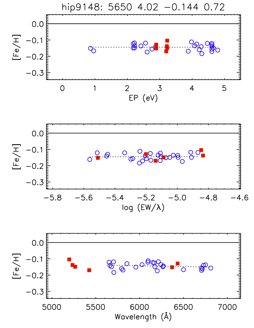
Figure 3: Measured iron abundance as a function of excitation potential (top panel), reduced equivalent width (middle panel), and wavelength (bottom panel) for HIP 9148. Open circles (filled squares) correspond to Fe i (Fe ii) lines. Dotted lines are linear fits to the data. The legend on the top panel shows the star name followed by the derived parameters: $T_{\mathrm{eff}}$, $\log g$, $\mathrm{[Fe/H]}$, and $v_{t}$. The solid line is at solar metallicity.

We started by using the standard iron line spectroscopic approach, which forces excitation and ionization balance of iron lines. A first guess of the parameters is made and iron abundances are computed for a number of neutral (Fe i) and singly ionized (Fe ii) iron lines. The parameters are then fine-tuned to remove any correlation between iron abundance and excitation potential (EP) of Fe i lines (therefore forcing excitation balance) and to minimize the difference between the mean iron abundances inferred from Fe i and Fe ii lines separately (thus achieving ionization balance). Simultaneously, the correlation between Fe i abundance and line strength is controlled (i.e., the correlation is minimized) with the microturbulent velocity parameter ($v_{t}$). Fig. 3 shows an example of the end product of this procedure. The iron line-list adopted (including atomic data) is from Asplund et al. (2009), who made a careful selection of unblended features for their solar abundance analysis. The abundances used in this procedure are differential, on a line-by-line basis, using the solar abundances inferred from our solar (Hebe) spectrum as reference. We adopted $v_{t}^{\odot}=1.0$ km s^-1, although the exact value of $v_{t}^{\odot}$ has a minor impact on our results.

Errors in the derived parameters are estimated from the uncertainty in the abundance versus EP slope (for $T_{\mathrm{eff}}$) and the line-to-line scatter of the mean Fe i and Fe ii abundances (for $\log g$). Since we force the EP slope to be zero, a slightly positive (negative) EP slope implies a $T_{\mathrm{eff}}$ too low (high) by a certain amount. We use the $\Delta T_{\mathrm{eff}}$ amount that corresponds to an EP slope of $\pm 1\sigma$, where $\sigma$ is the error of the zero slope when using the adopted $T_{\mathrm{eff}}$. For the error in $\log g$, we consider the maximum and minimum $\log g$ values such that the mean Fe i $-$ Fe ii abundance difference is consistent with zero within the $1\sigma$ line-to-line scatter as the upper and lower limits of the derived $\log g$.

A second set of parameters was obtained using colors to derive $T_{\mathrm{eff}}$. The recent metallicity-dependent color calibrations by Casagrande et al. (2010) for the following color indices: $B-V$, $b-y$, $V-J$, $V-H$, $V-K_{s}$, and $J-K_{s}$, were used. Observed magnitudes and colors of our sample stars were taken from the General Catalogue of Photometric Data (Mermilliod et al., 1997) and the 2MASS and Hipparcos/Tycho catalogs. We made sure that the adopted photometry was not blended (i.e., we excluded mainly old measurements for the unresolved systems) and avoided uncertain 2MASS photometry for the brightest stars. We did not apply the Casagrande et al. (2010) formulas to giant stars because their work is restricted to dwarf and subgiant stars. Errors in the photometry and the color-to-color $T_{\mathrm{eff}}$ scatter provides us with an estimate of the error in $T_{\mathrm{eff}}$. Photometric errors are simply propagated into the color$-T_{\mathrm{eff}}$ relations to obtain the error in $T_{\mathrm{eff}}$ for a given color. Then these errors are used as weights when computing the final $T_{\mathrm{eff}}$ value. The $T_{\mathrm{eff}}$ error is obtained using the formula for the sample variance, again using the $T_{\mathrm{eff}}$ errors for each color as weights.

Given a photometric $T_{\mathrm{eff}}$, the surface gravity was determined using two methods. The first one is the same as in the iron line analysis, i.e., $\log g$ is fine-tuned so that the mean iron abundances from Fe i and Fe ii lines agree (ionization balance). In the second case we determine $\log g$ using the stars’ trigonometric parallax from the new reduction of Hipparcos data (van Leeuwen, 2007) and theoretical isochrones. This method is described in detail in § 4. Note that in this latter case it is not guaranteed that the iron abundances inferred from Fe i and Fe ii lines are the same. Moreover, either if $\log g$ is inferred forcing ionization balance or using isochrones, the Fe i abundances will in general show a correlation with EP. Thus, the line-to-line scatter of the iron abundances inferred using photometric temperatures will be larger than that obtained by forcing excitation and ionization balance of iron lines. However, this does not imply a superiority of one method over another; it simply reflects the nature of the different approaches to measure the stellar parameters.

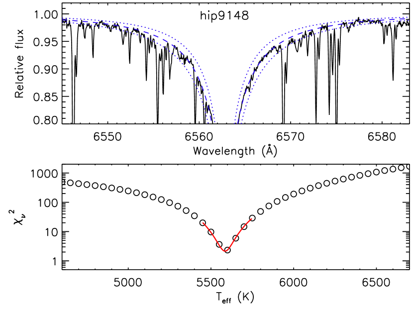
Figure 4: Top panel: Observed (solid line) and theoretical (dashed and dotted) H$\alpha$ line profiles for HIP 9148. The dashed line corresponds to the best fit $T_{\mathrm{eff}}$ H$\alpha$ model while dotted lines show profiles for $T_{\mathrm{eff}}\pm 200$ K. Bottom panel: reduced $\chi^{2}$ of observation minus model differences as a function of model $T_{\mathrm{eff}}$ (open circles). Only the regions not affected by narrow spectral lines are used in this computation. The solid line is a parabolic fit to the 7 points closest to the minimum, which allows a better $\chi^{2}$ minimization.

Finally, a third estimate of effective temperature can be obtained by analyzing the wings of Balmer lines, in particular H$\alpha$. The depth of these wings is highly sensitive to $T_{\mathrm{eff}}$ and if the other stellar parameters can be constrained independently, very precise $T_{\mathrm{eff}}$ values can be inferred from a $\chi^{2}$ minimization of observation minus theoretical models of H$\alpha$ line profiles (e.g., Barklem et al., 2002; Ramírez et al., 2006; Ramírez et al., 2011). A proper continuum normalization is required for this method to provide accurate effective temperatures. Our H$\alpha$ line profiles were normalized taking advantage of the smooth variation of the blaze function across spectral orders. Polynomial fits were used to trace the upper envelopes of spectral orders above and below the order containing the H$\alpha$ line. They were then interpolated to trace the continuum of the H$\alpha$ order. We used a grid of theoretical H$\alpha$ line profiles computed by Barklem et al. (2002), which is based on MARCS atmospheric models and the self-broadening theory developed in Barklem et al. (2000). A $\chi^{2}$ minimization routine allowed us to find the best model fits to our data and therefore to estimate $T_{\mathrm{eff}}$ and its associated error. Fig. 4 illustrates this technique. We obtained $T_{\mathrm{eff}}=5741\pm 40$ K for our solar (Hebe) spectrum, in very good agreement with the solar $T_{\mathrm{eff}}$ inferred by Barklem et al. (2002) using the H$\alpha$ line from the very high quality solar spectrum by Kurucz et al. (1984). The fact that the H$\alpha$ temperature of the Sun does not perfectly agree with the nominal value of 5777 K suggests that there is still room for improvement in the modeling of Balmer lines. We increased the $T_{\mathrm{eff}}$ values derived from our H$\alpha$ analysis by 36 K as a first order correction, given that this brings the solar $T_{\mathrm{eff}}$ up to its expected value. Similar to the case of photometric $T_{\mathrm{eff}}$, once the effective temperature was determined from the H$\alpha$ line analysis, we derived $\log g$ values using ionization balance as well as isochrones.

Note that all the methods described above require a previous knowledge of the atmospheric parameters, which are the quantities we want to derive. Thus, iterative procedures are necessary to obtain a final, self-consistent solution for the $T_{\mathrm{eff}},\log g,\mathrm{[Fe/H]}$ set. We repeated all calculations as many times as necessary to guarantee that no more iterations are required to improve these solutions.

The $T_{\mathrm{eff}}$, $\log g$, $\mathrm{[Fe/H]}$ values derived using the various techniques described in this Section are listed in Table Towards precise ages for single stars in the field. Gyrochronology constraints at several Gyr using wide binaries. I. Ages for initial sample.

3.3 Adopted Parameters

All methods of atmospheric parameter determination have limitations. For example, the excitation/ionization balance of iron lines assumes local thermodynamic equilibrium (LTE), which is a useful but not necessarily correct assumption (e.g., Asplund, 2005). Photometric temperature scales have uncertain zero points, and even though they seem to agree well with $T_{\mathrm{eff}}$ scales based on interferometric observations of stellar angular diameter, the latter are typically based on the analysis of giant stars, whose surfaces are far from being static and well-defined, as it is assumed in the measurement of angular diameters (e.g., Koesterke et al., 2008; Chiavassa et al., 2010). Also, the modeling of H$\alpha$ line profiles relies heavily on the theory of self-broadening, and different prescriptions may lead to significantly different results, as explored in detail by Barklem et al. (2002). Surface gravity determinations based on ionization balance rely also on the assumption of LTE while the isochrone approach depends on stellar structure and evolution calculations and may be affected by statistical biases (e.g., Pont & Eyer, 2004; Jørgensen & Lindegren, 2005).

It is therefore not surprising to find differences in the stellar parameters derived with different methods for the same object in Table Towards precise ages for single stars in the field. Gyrochronology constraints at several Gyr using wide binaries. I. Ages for initial sample. Our sample size is too small and it covers too wide of a region of stellar parameter space for us to clearly uncover systematic differences between the different methods. In any case, discrepant values typically point to systematic errors affecting differently each technique whereas values in good agreement suggest that the impact of these errors is relatively small. Thus, by taking the average value of all the measurements reported in Table Towards precise ages for single stars in the field. Gyrochronology constraints at several Gyr using wide binaries. I. Ages for initial sample for each object we improve upon values that are only slightly affected by systematic errors while assigning realistic error bars to stars for which their derived parameters likely suffer from severe systematic errors.

Our adopted parameters are obtained as the weighted average of all measurements available to each star. However, effective temperature errors lower than 35 K were set to 35 K before averaging. Similarly, the lowest adopted $\log g$ and $\mathrm{[Fe/H]}$ errors were 0.03 and 0.04 dex, respectively. This was done to avoid giving too much weight to a particular value. Small internal errors can in many cases be the result of numerical artifacts that do not reflect the true errors of the measurement. By adopting reasonable minimum errors we obtain more reliable, and therefore accurate, average values.

The errors adopted are the linear sum of the standard error and the sample variance. The first term takes into account the random errors of each measurement assuming that there are no systematic differences between the various values. The sample variance, on the other hand, is sensitive to systematic differences. Thus, by adding the sample variance to the standard error a more realistic error bar is obtained.

Our adopted parameters and their associated errors, computed as described in this Section, are given in Table Towards precise ages for single stars in the field. Gyrochronology constraints at several Gyr using wide binaries. I. Ages for initial sample.

4 Stellar ages

We compute the ages of our initial sample of recently evolved wide binaries by making use of theoretical isochrones. In this technique, the star under study is placed on a CMD and its location compared to theoretical predictions of stellar evolution. Isochrone points close to the observed stellar parameters are then used to derive the mass and age of the star (e.g., Lachaume et al. 1999). While the location of any star on the CMD is determined just by its absolute luminosity $M_{\rm V}$ and surface temperature $T_{\rm eff}$ (or color), many combinations of stellar parameters ($\log g$, [Fe/H], mass, and age) can go through that point, so that in order to infer the age of the star some of these parameters must also be given. Typically, the fundamental atmospheric parameters $T_{\rm eff}$, $\log g$, and [Fe/H] are measured from the star’s spectrum, photometry, or a combination of both (§ 3), and they are enough to determine both the age and mass of the star via isochrones. In our case, given that for some stars different methods to estimate $\log g$ produced discrepant answers (§ 3.3), we avoid this parameter and instead use the luminosity of the star, $M_{\rm V}$ (i.e., determined by its apparent magnitude and parallax).

In order to determine which isochrone fits best any particular star, we build the probability distribution of the stellar age by computing the likelihood that any given isochrone passes near the corresponding set of stellar parameters, accounting for the uncertainties on those parameters. The age probability distribution is also called the “G function”, and the procedure is widely used nowadays (e.g., Lachaume et al. 1999; Reddy et al. 2003; Nordstrom et al. 2004; Allende Prieto et al. 2004; Pont & Eyer 2004). Assuming the errors in our stellar parameters ($\sigma_{T_{\rm eff}}$, $\sigma_{\rm[Fe/H]}$, and $\sigma_{M_{\rm V}}$) have Gaussian probability distributions, the likelihood for a point in a given isochrone can be written as

$$P(T_{\rm eff},{\rm[Fe/H]},M_{\rm V})\propto\exp\left[-(\Delta T_{\rm eff})^{2}\over 2\sigma_{T_{\rm eff}}^{2}\right]\exp\left[-(\Delta[{\rm Fe/H}])^{2}\over 2\sigma_{[{\rm Fe/H}]}^{2}\right]\exp\left[-(\Delta M_{\rm V})^{2}\over 2\sigma_{M_{\rm V}}^{2}\right],$$ (1)

where $\Delta T_{\rm eff}$, $\Delta[{\rm Fe/H}]$, and $\Delta M_{\rm V}$ are the differences between the measured stellar parameters and those corresponding to the point in the isochrone under consideration. The integral of this likelihood over all the parameter space of the set of isochrones then gives the age probability distribution

$$P({\rm age})=\int P(T_{\rm eff},{\rm[Fe/H]},M_{\rm V})\,{\rm d}T_{\rm eff}\,{\rm d[Fe/H]}\,{\rm d}M_{\rm V}.$$ (2)

In practice, we only integrate over the volume defined by three times the $1\sigma$ uncertainties from the measured stellar parameters, which we verified already accounts for most of the contribution to the probability distribution from the entire set of isochrones. Being the most likely value, we then adopt the peak of the G-function as the age of the star.

The choice on how to determine the exact location of the peak of the G-function has a small effect on the adopted age, especially given the size of our $1\sigma$ errors, typically larger than $\sim$ 0.5 Gyr. Therefore, we do not implement at this point anything more sophisticated than just adopting as our age the center of the bin where the peak occurs, and leave for a later stage in this program any refinement, if at all needed. Due to the discrete nature of the procedure of isochrone fitting, this lack of “smoothing” of the G-functions leads to the appearance of spurious structure in the distribution of ages of large samples of stars (e.g., Nordstrom et al. 2004), so a more sophisticated approach to determine the exact location of the peak is relevant for population studies, which is not the case here.

As an illustration, Figure 5 shows the resulting age distributions and $1\sigma$ uncertainties around the most likely age for the pair HIP 115126/NLTT 56465 (solid lines). We normalize the distributions so that the area below is equal to 1. The adopted errors are computed from the cumulative function of the age probability distribution (dashed lines), assuming the latter is well approximated by a Gaussian. However, as is clear from the bottom panel in Figure 5, this G-function is not always close to a Gaussian, and thus we adopt different $1\sigma$ errors to both sides of the peak. Our $1\sigma$ lower and upper limits mark the age interval of cumulative probability between 16% and 84%.

Using this procedure we compute the ages of all stars (both primaries and secondaries) in our initial sample. We use Yale-Yonsei isochrones (Yi et al., 2001; Demarque et al., 2004) sampled with constant steps of 0.1 Gyr in age and 0.02 dex in [Fe/H], covering ages from 0.1 to 15 Gyr. In constructing the age probability distribution, we experimented with different bin sizes and found that 0.5 Gyr/bin was an optimal choice and smaller bins did not change the resulting ages. For the case of binaries with both components in Hipparcos, we adopt for both stars the primary’s parallax, which for all pairs in this category is the one with the better measurement (i.e., smaller error). The resulting ages and uncertainties for all stars that could be observed with enough signal-to-noise are listed in Table 7

Following the same steps leading to the derivation of the isochronal age via equations 1 and 2, one can derive an isochronal $\log g$ through the construction of the gravity probability distribution. Our results for this isochronal $\log g$ are listed in Table Towards precise ages for single stars in the field. Gyrochronology constraints at several Gyr using wide binaries. I. Ages for initial sample (labeled as $\log g_{\rm iso}$), where they can be compared to the average of the resulting $\log g$ derived from all other methods. Since the $\log g_{\rm iso}$ are obtained from our final $T_{\rm eff}$ and [Fe/H] for each star, as listed also in Table Towards precise ages for single stars in the field. Gyrochronology constraints at several Gyr using wide binaries. I. Ages for initial sample, they are our preferred values, above the $\log g$ obtained as the average of different methods in Section 3.

Next we consider the interesting possibility of improving the ages of those systems in our sample for which the two components were able to provide an independent age. In these cases, since both components contain some information on the age of the system, instead of treating them independently we can treat them simultaneously by forcing the procedure of isochrone fitting to consider the two stars as coeval. This can be done by computing the age probability distribution of the binary system, which would be given by

$$P({\rm age})=\int P_{\rm A}\,P_{\rm B}\,{\rm d}T_{\rm eff}\,{\rm d[Fe/H]}\,{\rm d}M_{\rm V},$$ (3)

where $P_{\rm A}$ and $P_{\rm B}$ are the likelihoods for components A and B, respectively, and given by equation 1. While equation 3 gives the same weight to both stars, one could assign different weights based on a number of criteria, but we choose to not attempt this. Figure 6 illustrates the case of HIP 115126/NLTT 56465, the same pair shown in Figure 5. The net effect of considering the two components simultaneously was to shift the entire G-function of the evolved primary towards younger ages, closer to the broad peak of the secondary’s G-function. The nominal precision of the resulting combined age (i.e., the size of the $1\sigma$ region around the peak), however, remains esentially the same as that for the evolved primary alone.

All the ages derived up to this point come directly from the adopted set of isochrones and the fitting procedure detailed above. The use of a different set of isochrones will, in principle, change our results. Moreover, isochrone ages are known to suffer from a number of systematic biases arising, for example, from the fact that, due to the different timescales characteristic of different evolutionary stages, isochrones do not evenly map the relevant parameter space of stellar parameters. There is a significant literature on the subject of such age biases and the available ways to correct for them (Pont & Eyer, 2004; Nordstrom et al., 2004; Jørgensen & Lindegren, 2005). These systematics are important when dealing with large samples of stars and attempting to extract conclusions of a statistical nature, such as those related to the age-metallicity relation in the solar neighborhood (e.g., Casagrande et al. 2011). Since the main purpose of the present paper is to introduce our program for gyrochronology with wide binaries and demonstrate that precise ages (i.e., with reasonably small internal errors) can be achieved for them, any refining of the ages derived in this section will be attempted later, if at all necessary, and thus we do not implement any corrections for statistical biases or derive ages from other isochrone grids at this point.

Nevertheless, in order to provide readers with a quantitative idea of the differences expected when accounting for statistical biases and isochrone grid choice, we compute the ages obtained by making use of the “web interface for the Bayesian estimation of stellar parameters”, maintained at the Osservatorio Astronomico di Padova and described in da Silva et al. (2006). This publicly available tool uses a different set of isochrones than the one used in this paper (namely, that by Girardi et al. 2000) and accounts for some of the biases discussed above. The tool requires the selection of priors for the Bayesian analysis, for which we choose an initial mass function from Chabrier (2001), and a constant star formation rate in the interval from 1 to 12 Gyr. The resulting ages and their uncertainties are listed in Table 7 next to our own determinations.

In Figure 7a we show the comparison between our isochronal ages (for the components of the wide binaries treated independently) and those obtained accounting for statistical biases following the da Silva et al. (2006) prescription and a different set of isochrones. In most cases the ages are remarkably similar, even in the adopted uncertainties. The mean difference of the maximum likelihood ages, for the cases where the da Silva et al. (2006) ages are at least three times larger than their $1\sigma$ errors, is only $0.1\pm 0.6$ Gyr, thus giving reliability to our isochronal ages and suggesting that inclusion of the statistical biases is not crucial for our purposes.

We also tested our age determination method against the Bayesian implementation by Casagrande et al. (2011, hereafter C11). They derived improved stellar parameters and ages of all stars in the Geneva-Copenhagen Survey (GCS, Nordstrom et al. 2004). We selected a small sub-sample of 47 GCS stars from C11. These stars have ages with errors smaller than 16 % if young ($<2.8$ Gyr) and smaller than 20 % otherwise ($>2.8$ Gyr), as given by C11. We used the effective temperatures and metallicities given by C11 along with the stars’ visual magnitudes and Hipparcos parallaxes to derive ages using our isochrone-fitting program, i.e., we used the exact same input data employed by C11. Figure 7b shows the comparison of C11 and our ages for this small sample. The agreement between the two sets of ages is excellent, with a mean difference of only $0.03\pm 0.45$ Gyr. A closer inspection of this Figure suggests very small systematic differences. For stars older than 7 Gyr, our ages are slightly younger ($-0.48\pm 0.33$ Gyr) whereas for stars younger than 4 Gyr they appear slightly old (although the mean difference is still consistent with zero: $0.2\pm 0.4$ Gyr). In this test we employed the ages from C11 derived using Padova isochrones. A similar test using the ages they derived with BASTI isochrones (e.g., Pietrinferni et al. 2004, 2006) gives almost the same result. Thus, we show again that statistical biases and the choice of isochrone grid appears to have a minor impact on our project.

5 Summary and Conclusions

We have started a program that takes advantage of wide binaries with evolved components and solar-type main-sequence companions in order to obtain constraints for the calibration of age-rotation relations (gyrochronology) at ages of several Gyr. We have mined published catalogs of wide binaries and assembled a sample of 38 wide binary systems with either turnoff/subgiant (20) or white dwarf (18) components that are well positioned to provide ages for these systems. For an initial subsample comprised of 15 of the binaries with turnoff or subgiant components we measured precise stellar parameters from high resolution optical spectra, and used these results to derive ages for the binary systems using theoretical isochrones. As judged from a one-to-one comparison with results obtained by state-of-the-art analysis that takes into account a number of known systematics of the isochrone technique, our own isochronal ages and the adopted uncertainties appear to be robust. We obtained the ages of 16 of our 18 systems with white dwarf components directly from the literature, having been derived from models of white dwarf cooling and empirically-calibrated initial-to-final-mass relationships.

The ages of the 31 wide binary systems provided in this work range from 1 to 9 Gyr. At least 15 of these systems have $1\sigma$ uncertainties of about 0.5 Gyr or less. Those for which the rotation period of the main sequence companion is suitable to be measured will thus provide useful constraints for gyrochronology relations, in a regime of ages where the only constraint currently available is that provided by the Sun. Observations aimed at the measurement of the rotation periods of these stars have started and will be reported in a future paper.

As larger and more varied samples of wide binaries start to become available thanks to ongoing and planned all-sky surveys, the potential of programs like the one presented in this paper for the purposes of gyrochronology will only increase. Taking advantage of the SUPERBLINK survey (Lépine, 2008), we have already more than doubled the sample reported in Tables 1 to 3, and observations aimed to derive their ages are scheduled. With the help of increasingly improving photometric distances and stellar parameters, it may be possible today or in the near future to extend this work to the fainter database of the Sloan Digital Sky Survey. Finally, the unprecedented scale, depth, and precision levels of the data expected from upcoming projects like Gaia and LSST will provide large quantities of wide binary systems suitable not only for gyrochronology but for a large range of other applications (Chanamé, 2007).

Figure 1: Selection of wide binary pairs with turnoff/subgiant components, both members having independent Hipparcos parallaxes (primaries as filled symbols, secondaries as open symbols). The 9 pairs in this category are shown here on two different color-magnitude diagrams and listed in Table 1. The small background dots in the $B-V$ CMD are Hipparcos single stars within 100 pc of the Sun and with better than $5−\sigma$ parallaxes, and in the $V-J$ CMD they are single Hipparcos stars in the LSPM catalog and within 33 pc of the Sun (Lépine 2005). Primaries within the dashed area in the $B-V$ CMD and with main-sequence secondaries bluer than $B-V=1.40$ are selected for further inspection.

.

Figure 2: Same as Figure 1, but for pairs with only one Hipparcos component. The 10 pairs shown here are listed in Table 2. Primaries within the dashed area in the $B-V$ color-magnitude diagram and with main-sequence secondaries bluer than $V-J\sim 3.0$, approximately the boundary between K and M dwarfs, are selected for further inspection. The magnitudes of a few pairs have been randomized by a small amount in order to avoid clutter. Due to lack of colors in some cases, not all of the MS secondaries can be shown. Note in the upper panel the pair composed of a turnoff/subgiant primary and a WD secondary (HIP 18824/NLTT 12412, with the WD located at M${}_{\rm V}\sim 14$ and $V-J\sim 1$). Even though there is no FGK MS star in this pair, we keep it in our program in case the WD is of DA type in order to compare the age of the same system obtained from two different methods.

.

Figure 5: Age probability distributions (solid lines) for the components of a representative case (not the best, not the worst) of our initial sample of wide binaries with recently evolved components. The vertical dotted lines indicate the location of the adopted $1\sigma$ errors to both sides of the peak of the distributions, obtained from the cumulative function of the age distribution (dashed lines). The evolved primary provides a significantly better constraint on the age than the MS secondary.

Figure 6: Age probability distribution assuming coevality for the pair shown in Figure 5, i.e., considering the two components simultaneously (see text in § 4). Upper panel: independent, single-star age probability distributions for HIP 115126 (A, primary) and NLTT 56465 (B, secondary). Lower panel: Joint probability distribution (solid line), obtained by forcing the isochrone fitting to pass through the two components of the binary using equation 3.

Figure 7: (a) Direct comparison between the isochronal ages derived in this work and those obtained using the da Silva et al. (2006) prescription, which accounts for statistical biases and makes use of a different set of isochrones. The filled circles are stars considered robust by da Silva et al. (2006) (age/$\sigma_{\rm age}>3$). The agreement is excellent, with only $3-4$ significantly discrepant cases out of a total of 24 stars. (b) Comparison of ages from the GCS survey for a small sample of GCS stars with very well determined ages, as derived by Casagrande et al. (2011) and our ages, obtained using the exact same input data from C11.

Table 1: Wide binaries with recently evolved primaries, both stars in Hipparcos.

HIP	$\mu_{\rm RA}$	$\mu_{\rm DEC}$	$\pi$	$\sigma_{\pi}$	$V$	$B-V$	$V-J$	Sp.Type1	$\Delta\theta$	$\Delta\mu$	NLTT/LSPM	Comments
	(mas/yr)	(mas/yr)	(mas)	(mas)	(mag)	(mag)	(mag)		(arcsec)	(mas/yr)
9243	137.5	125.9	7.81	0.79	8.27	0.88	1.64	K0IV	36.0	3.5	6664
9247	138.0	129.4	7.82	0.94	9.11	0.54	1.02	F8			6665
10305	378.2	-70.6	21.71	1.67	5.65	0.55	0.60	F8V	16.7	5.5	7323
10303	383.5	-72.2	20.89	7.39	7.56	0.72	1.03	G4			7321
58240	-174.0	-5.3	21.13	6.41	7.80	0.67	1.31	G3V	18.8	6.9	29039	pre-MS star1
58241	-180.9	-5.4	8.35	6.35	7.83	0.64	1.23	G4V			29041
74432	-594.9	296.3	36.71	1.91	6.69	0.68	1.23	G5V	23.4	12.8	39601	secondary within box
74434	-594.9	283.5	21.49	4.98	7.71	0.74	1.47	G7V			39603
81991	-215.7	-257.7	21.80	0.91	6.55	0.89	1.61	G5	163.0	4.5	43483
81988	-219.3	-255.0	23.06	1.73	10.31	1.04	2.01	K3			43481
94076	51.7	186.1	19.11	1.57	6.70	0.64	1.15	G1V	15.9	20.3	47474	spectroscopic binary1
94075	69.1	196.6	23.48	4.95	7.97	0.75	1.22	G5			47473	substellar companion
101916	322.2	21.2	33.20	0.82	5.07	0.70	0.96	G5IV	214.0	4.5	49632
101932	317.8	20.1	34.90	1.14	8.52	0.91	1.58	K2V			49639
101082	68	221	15.69	0.50	5.97	0.94	1.47	K0III	214.2	1.0	J2029+8105
101166	68	220	14.51	0.70	8.68	0.64	1.13	G5			J2030+8108
102532	-30	-198	25.82	1.20	4.25	1.04	0.97	K1IV	9.1	29.6	J2046+1607E
102531	-1	-204	26.35	2.40	4.97	0.49	2.91	F7V			J2046+1607W

Note. — (1) Obtained from the SIMBAD database.

Table 2: Wide binaries with recently evolved primaries, only primary star in Hipparcos.

HIP	NLTT/LSPM	$\mu_{\rm RA}$	$\mu_{\rm DEC}$	$\pi$	$\sigma_{\pi}$	$V$	$B-V$	$V-J$	Sp.Type1	$\Delta\theta$	$\Delta\mu$	Comments
		(mas/yr)	(mas/yr)	(mas)	(mas)	(mag)	(mag)	(mag)		(arcsec)	(mas/yr)
9148	6581	214	50	11.15	1.11	8.26	0.70	1.26	G3V	41.5	5
	6583	219	52			13.07	9.99	2.29
18824	12415	373	-12	19.35	0.63	6.80	0.63	1.17	G1V	64.1	4
	12412	370	-12			17.82	9.99	0.99				white dwarf
23926	14574	-73	289	18.69	0.49	6.75	0.66	1.24	G3V	10.0	16
	14573	-64	276	18.46	0.65	10.11	0.67	1.62	G0			HIP 23923
32935	17118	123	156	8.19	0.57	8.12	0.94	1.74	K0IV	46.1	2
	17117	123	154			10.11	0.55	1.09	G0
114855	56282	370	-17	21.77	0.29	4.24	1.11	1.98	K0III	49.6	14	giant; substellar companion
	56278	370	-17			9.73	1.06	2.42	K3
115126	56466	266	-45	47.35	2.47	5.20	0.79	1.38	G8.5IV	12.2	32
	56465	266	-45			8.88	0.88	2.84	K2V
18448	J0356+6950	190	-168	6.44	1.20	9.34	0.93	1.68	K0	24.7	1
	J0356+6951	189	-167			14.72	9.99	2.52
6914	J0129+7412W	194	-121	17.89	0.60	7.26	0.67	1.23	G5	27.0	42
	J0129+7412E	183	-80			12.61	1.17	2.89
20197	J0419+1416	82	-216	11.89	1.10	7.54	0.99	1.81	G7III	215.0	14
	J0419+1419	87	-203			13.12	0.75	2.74				possibly M dwarf
107759	J2149+1402S	159	-41	5.78	1.50	9.65	0.74	1.41	G5	13.3	9
	J2149+1402N	154	-33			99.99	9.99	9.99

Note. — (1) Obtained from the SIMBAD database.

Table 3: Wide binaries with white dwarf components.

NLTT	$\mu_{\rm RA}$	$\mu_{\rm DEC}$	$\pi$	$\sigma_{\pi}$	$V$	$B-V$	$V-J$	Sp.Type1	$\Delta\theta$	$\Delta\mu$	Age	Comments
	(mas/yr)	(mas/yr)	(mas)	(mas)	(mag)	(mag)	(mag)		(arcsec)	(mas/yr)	(Gyr)
1762	207	-53			16.59	0.30	-0.078	DA	28.8	18	1.2${}^{+0.15}_{-0.14}$
1759	222	-44	9.52	1.63	10.28	0.78	1.475	K1				HIP 2600
29967	-299	-328			17.26	9.99	1.19	DA	202.8	15
29948	-292	-313	22.94	1.63	9.96	0.99	1.89	K4				HIP 59519
13599	228	-155			15.94	0.65	1.34	DA/DC	123.9	8	5.4${}^{+2.6}_{-1.3}$
13601	233	-149	56.02	1.21	8.42	1.10	2.47	K7				HIP 21482
55288	548	-57			16.50	0.42	0.87	DA	41.8	9	3.6${}^{+2.1}_{-0.9}$
55287	551	-49	28.72	1.30	8.03	0.66	1.22	G7				HIP 113231
44348	-92	252			17.50	0.10	9.99	DA/DF	28.7	8
44344	-88	259	18.18	1.35	11.46	1.02	2.34	K7				phot plx
7890	-116	-145			17.39	-1.19	1.24	DA	40.5	10	5.0${}^{+2.5}_{-1.2}$
7887	-119	-155	22.22	2.50	9.84	1.01	1.90	K3				phot plx
1374	72	-205			16.22	0.36	0.17	DA	59.2	2	2.3${}^{+1.6}_{-0.7}$
1370	74	-206	8.00	0.65	12.90	1.70	2.16	K6				phot plx
LP378-537					16.2			DA			$1.0^{+0.2}_{-0.1}$
BD+23 2539	-101	79	56.7		9.7	0.7422	1.252	K0	20
LP786-6	-190	33			15.7	-0.118	-0.552	DB			$2.0^{+0.8}_{-0.6}$	NLTT 20260
BD-18 2482			29.49		12.8	1.0362		K3	31
40 Eri B	-2228	-3377			9.5	0.11	-0.349	DA	82	45	$5.0^{+1.1}_{-1.0}$	NLTT 12868
40 Eri A	-2240	-3420	200.62	0.23	4.4	0.82	1.397	K1				NLTT 12863
L481-60	-415	-214	65.6		12.8	0.30		DA		1	$1.1^{+0.2}_{-0.2}$	NLTT 41169
CD-37 10500	-415	-215	65.13	0.40	6.0	0.72	1.051	G7IV	15			NLTT 41167
L182-61	-46	-316			14.1	-0.09	-0.214	DB		1	$1.4^{+1.0}_{-1.0}$	NLTT 16355
CD-59 1275	-46	-316	26.72	0.29	6.4	0.59	1.024	G0	41			NLTT 16354
CD-38 10980	76	1	76.00	2.56	11.0	-0.14	-0.548	DA		6	$1.4^{+0.9}_{-0.5}$	HIP 80300
CD-38 10983	72	5	78.26	0.37	5.4	0.597	0.966	G5	345			HIP 80337
LHS300B					17.8			DB			$7.9^{+1.1}_{-2.4}$
LHS300A			32.3		13.2			K
LP592-80					17.2			DA	49		$2.6^{+1.3}_{-1.3}$
BD-1 469	253	-60	14.89	0.84	5.4	1.04	1.966	K1IV				HIP 15383
G216-B14B					15.5			DA	23		$1.2^{+0.1}_{-0.2}$	B-band mag
G216-B14A					12.0		2.864
G116-16	38	-296	34.6	4.00	15.4	0.21	0.355	DA	1020	17	$1.6^{+0.2}_{-0.2}$	NLTT 21338
BD+44 1847	34	-279	19.0	1.04	9.0	0.68	1.315	G0				NLTT 21283
G273-B1B	169	7			16.4			DA	36		$3.4^{+0.8}_{-0.7}$
G273-B1A					11.0			G				B-band mag

Note. — (1) Spectral types are taken preferentially from the original source, i.e., either Garcés, Catalán, & Ribas (2011) or Zhao et al. (2011), or else from the SIMBAD database.

Table 4: Observing Log and Derived Radial Velocities

Object	UT date	UT time	Exp. time	S/N	Radial velocity
	(yyyy-mm-dd)	(hh:mm:ss)	(seconds)	$\lambda=6000$ Å	(km s-1)
Hebe	2010-09-21	04:10:27	1004	289	$\ldots$
HIP9148	2010-09-22	03:38:02	3648	420	$17.13\pm 0.25$
HIP9243	2010-09-21	04:47:48	2670	447	$7.84\pm 0.24$
HIP9247	2010-09-21	05:38:55	3250	314	$7.26\pm 0.50$
HIP10305	2011-01-04	01:43:37	138	479	$-3.81\pm 0.78$
HIP10303	2011-01-04	01:05:54	843	505	$-4.90\pm 0.25$
HIP18824	2010-09-21	08:48:35	2081	111	$10.64\pm 0.31$
HIP20197	2010-09-22	09:17:40	405	437	$-18.58\pm 0.31$
HIP23926	2010-09-21	06:48:54	435	409	$44.30\pm 0.30$
HIP23923	2010-09-21	07:08:18	4606	180	$45.27\pm 0.22$
HIP32935	2010-09-22	07:00:49	1725	378	$88.24\pm 0.32$
NLTT17117	2010-09-22	08:42:38	1800	236	$88.61\pm 0.40$
HIP74432	2010-09-21	23:16:51	180	211	$-39.03\pm 0.40$
HIP74434	2010-09-21	23:23:45	120	120	$-38.56\pm 0.36$
HIP81991	2010-09-20	23:31:06	150	270	$-5.29\pm 0.25$
HIP94076	2010-09-21	23:32:49	947	439	$-44.08\pm 0.43$
HIP94075	2010-09-21	23:55:35	2716	548	$-40.08\pm 0.41$
HIP101916	2010-09-21	00:54:04	90	513	$-53.89\pm 0.29$
HIP101932	2010-09-21	01:02:19	1200	451	$-52.43\pm 0.24$
HIP102532	2010-09-22	00:52:17	30	442	$-5.72\pm 0.32$
HIP102531	2010-09-22	00:59:06	75	443	$-6.56\pm 0.49$
HIP107759	2010-09-22	01:12:56	3112	286	$-63.95\pm 0.33$
HIP115126	2010-09-21	03:02:41	190	436	$8.49\pm 0.26$
NLTT56465	2010-09-21	03:16:26	1478	453	$11.55\pm 0.19$
HIP114855	2010-09-21	01:52:46	105	624	$-25.62\pm 0.28$
NLTT56278	2010-09-21	01:58:50	2400	276	$-22.88\pm 0.36$

Table 5: Measured Stellar Parameters

Table 6: Adopted Stellar Parameters

Table 7: Isochronal ages for wide binaries with turnoff and subgiant components

ID	this work	da Silva et al. (2006)
	(Gyr)	(Gyr)
HIP 9148	6.75${}^{+1.57}_{-1.32}$	7.776 $\pm$ 1.744
NLTT 6583
HIP 9243	3.25${}^{+0.67}_{-0.59}$	2.790 $\pm$ 0.423
HIP 9247	5.25${}^{+0.11}_{-1.20}$	5.594 $\pm$ 0.995
HIP 10305	2.75${}^{+0.50}_{-0.33}$	2.587 $\pm$ 0.326
HIP 10303	7.75${}^{+0.62}_{-2.03}$	4.832 $\pm$ 3.710
HIP 18824	4.75${}^{+0.47}_{-0.21}$	4.672 $\pm$ 0.483
NLTT 12412
HIP 20197	6.25${}^{+2.55}_{-1.04}$	5.559 $\pm$ 1.573
LSPM J0419+1419
HIP 23926	4.75${}^{+0.17}_{-0.57}$	4.674 $\pm$ 0.332
HIP 23923	5.75${}^{+6.92}_{-2.34}$	4.381 $\pm$ 3.980
HIP 32935	8.75${}^{+4.00}_{-2.07}$	7.891 $\pm$ 2.262
NLTT 17117	9.75${}^{+1.29}_{-3.13}$	8.665 $\pm$ 3.655
HIP 74432	7.75${}^{+1.39}_{-1.78}$	7.968 $\pm$ 2.045
HIP 74434	2.25${}^{+4.92}_{-0.77}$	8.384 $\pm$ 3.618
HIP 81991	4.75${}^{+3.56}_{-0.06}$	5.949 $\pm$ 1.636
HIP 81988
HIP 94076	4.25${}^{+0.47}_{-0.66}$	3.490 $\pm$ 0.684
HIP 94075	8.75${}^{+1.32}_{-2.87}$	4.463 $\pm$ 3.920
HIP 101916	3.25${}^{+0.19}_{-0.22}$	2.944 $\pm$ 0.105
HIP 101932	6.25${}^{+4.75}_{-3.13}$	3.655 $\pm$ 3.632
HIP 102532	1.25${}^{+0.21}_{-0.32}$	1.114 $\pm$ 0.128
HIP 102531	2.75${}^{+0.10}_{-0.77}$	1.774 $\pm$ 0.154
HIP 107759	6.25${}^{+5.70}_{-1.72}$	7.130 $\pm$ 2.977
LSPM J2149+1402N
HIP 115126	6.25${}^{+0.93}_{-0.65}$	6.115 $\pm$ 0.869
NLTT 56465	3.25${}^{+5.67}_{-1.32}$	3.699 $\pm$ 3.563
HIP 114855	1.25${}^{+0.16}_{-0.34}$	1.460 $\pm$ 0.260
NLTT 56278		5.021 $\pm$ 3.957

References

- Abadi et al. (2003) Abadi, M. G., Navarro, J. F., Steinmetz, M., & Eke, V. R. 2003, ApJ, 597, 21
- Allende Prieto et al. (2004) Allende Prieto, C., Barklem, P. S., Lambert, D. L., & Cunha, K. 2004, A&A, 420, 183
- Asplund (2005) Asplund, M. 2005, ARA&A, 43, 481
- Asplund et al. (2009) Asplund, M., Grevesse, N., Sauval, A. J., & Scott, P. 2009, ARA&A, 47, 481
- Baliunas et al. (1983) Baliunas, S. L., Hartmann, L., Noyes, R. W., et al. 1983, ApJ, 275, 752
- Barklem et al. (2000) Barklem, P. S., Piskunov, N., & O’Mara, B. J. 2000, A&AS, 142, 467
- Barklem et al. (2002) Barklem, P. S., Stempels, H. C., Allende Prieto, C., Kochukhov, O. P., Piskunov, N., & O’Mara, B. J. 2002, A&A, 385, 951
- Barnes (2003) Barnes, S. 2003, ApJ, 586, 464
- Barnes (2007) Barnes, S. 2007, ApJ, 669, 1167
- Barnes (2010) Barnes, S. 2010, ApJ, 722, 222
- Baumann et al. (2010) Baumann, P., Ramírez, I., Meléndez, J., Asplund, M., & Lind, K. 2010, A&A, 519, A87
- Bernstein et al. (2003) Bernstein, R., Shectman, S. A., Gunnels, S. M., Mochnacki, S., & Athey, A. E. 2003, Proc. SPIE, 4841, 1694
- Brook et al. (2007) Brook, C., Richard, S., Kawata, D., Martel, H., & Gibson, B. K. 2007, ApJ, 658, 60
- Casagrande et al. (2010) Casagrande, L., Ramírez, I., Meléndez, J., Bessell, M., & Asplund, M. 2010, A&A, 512, 54
- Casagrande et al. (2011) Casagrande, L., Schönrich, R., Asplund, M., Cassisi, S., Ramírez, I., Meléndez, J., Bensby, T., & Feltzing, S. 2011, A&A, 530, A138
- Chabrier (2001) Chabrier, G. 2001, ApJ, 554, 1274
- Chanamé & Gould (2004) Chanamé, J. & Gould, A. 2004, ApJ, 601, 289
- Chanamé (2007) Chanamé, J. 2007, IAU Symposium, 240, 316
- Chiavassa et al. (2010) Chiavassa, A., Collet, R., Casagrande, L., & Asplund, M. 2010, A&A, 524, A93
- Cincunegui et al. (2007) Cincunegui, C., Díaz, R. F., & Mauas, P. J. D. 2007, A&A, 469, 309
- Csizmadia et al. (2011) Csizmadia, S., Moutou, C., Deleuil, M., et al. 2011, A&A, 531, A41
- Collier Cameron et al. (2009) Collier Cameron, A., Davidson, V. A., Hebb, L., et al. 2009, MNRAS, 400, 451
- Conroy & Wechsler (2009) Conroy, C., & Wechsler, R. H. 2009, ApJ, 696, 620
- Correia et al. (2006) Correia, S., Zinnecker, H., Ratzka, T., & Sterzik, M. F. 2006, A&A, 459, 909
- da Silva et al. (2006) da Silva, L., et al. 2006, A&A, 458, 609
- Delorme et al. (2011) Delorme, P., Collier Cameron, A., Hebb, L., et al. 2011, MNRAS, 413, 2218
- Demarque et al. (2004) Demarque, P., Woo, J.-H., Kim, Y.-C., & Yi, S. K. 2004, ApJS, 155, 667
- Desidera et al. (2004) Desidera, S., et al. 2004, A&A, 420, 683
- Dhital et al. (2010) Dhital, S., West, A. A., Stassun, K. G., & Bochanski, J. J. 2010, AJ, 139, 2566
- Garcés, Catalán, & Ribas (2011) Garcés, A., Catalán, S., & Ribas, I. 2011, A&A, 531, A7
- Giclas et al. (1971) Giclas, H. L., Burnham, R., & Thomas, N. G. 1971, Flagstaff, Arizona: Lowell Observatory, 1971
- Girardi et al. (2000) Girardi, L., Bressan, A., Bertelli, G., & Chiosi, C. 2000, A&AS, 141, 371
- Gould & Chanamé (2004) Gould, A., & Chanamé, J. 2004, ApJS, 150, 455
- Gray (2009) Gray, D. F. 2009, ApJ, 697, 1032
- Gustafsson et al. (2008) Gustafsson, B., Edvardsson, B., Eriksson, K., Jørgensen, U. G., Nordlund, Å., & Plez, B. 2008, A&A, 486, 951
- Hall, Lockwood, & Skiff (2007) Hall, J. C., Lockwood, G. W., & Skiff, B. A. 2007, AJ, 133, 862
- Hartman et al. (2009) Hartman, J. D., et al. 2009, ApJ, 691, 342
- Hartman et al. (2010) Hartman, J. D., Bakos, G. Á., Kovács, G., & Noyes, R. W. 2010, MNRAS, 408, 475
- Hartman et al. (2011) Hartman, J. D., Bakos, G. Á., Noyes, R. W., et al. 2011, AJ, 141, 166
- Irwin et al. (2006) Irwin, J., Aigrain, S., Hodgkin, S., Irwin, M., Bouvier, J., Clarke, C., Hebb, L., & Moraux, E. 2006, MNRAS, 370, 954
- Jørgensen & Lindegren (2005) Jørgensen, B. R., & Lindegren, L. 2005, A&A, 436, 127
- Koesterke et al. (2008) Koesterke, L., Allende Prieto, C., & Lambert, D. L. 2008, ApJ, 680, 764
- Kouwenhoven et al. (2010) Kouwenhoven, M. B. N., et al. 2010, MNRAS, 404, 1835
- Kurucz et al. (1984) Kurucz, R. L., Furenlid, I., Brault, J., & Testerman, L. 1984, Solar flux atlas from 296 to 1300 nm (National Solar Observatory Atlas, Sunspot, New Mexico: National Solar Observatory, 1984)
- Lachaume et al. (1999) Lachaume, R., Dominik, C., Lanz, T., & Habing, H. J. 1999, A&A, 348, 897
- Lépine (2005) Lépine, S. 2005, AJ, 130, 1680
- Lépine & Bongiorno (2007) Lépine, S., & Bongiorno, B. 2007, AJ, 133, 889
- Lépine (2008) Lépine, S. 2008, AJ, 135, 2177
- Luyten (1979) Luyten, W. J. 1979, Proper Motion Survey with the forty-eight inch Schmidt telescope. LII. Binaries with white dwarf components. White dwarf discovery? A travesty on the English language., by Luyten, W. J.. Separat print Univ. Minnesota, Minneapolis, Minnesota, 12 p., 52, 1
- Meibom et al. (2009) Meibom, S., Mathieu, R. D., & Stassun, K. G. 2009, ApJ, 695, 679
- Meibom et al. (2011a) Meibom, S., et al. 2011a, ApJ, 733, 115
- Meibom et al. (2011b) Meibom, S., et al. 2011b, ApJ, 733, L9
- Meléndez et al. (2009) Meléndez, J., Asplund, M., Gustafsson, B., & Yong, D. 2009, ApJ, 704, L66
- Mermilliod et al. (1997) Mermilliod, J., Mermilliod, M., & Hauck, B. 1997, A&AS, 124, 349
- Messina et al. (2008) Messina, S., Distefano, E., Parihar, P., Kang, Y. B., Kim, S.-L., Rey, S.-C., & Lee, C.-U. 2008, A&A, 483, 253
- Michaud et al. (2010) Michaud, G., Richer, J., & Richard, O. 2010, A&A, 510, A104
- Miller-Ricci et al. (2008) Miller-Ricci, E., Rowe, J. F., Sasselov, D., et al. 2008, ApJ, 682, 586
- Nagamine et al. (2005) Nagamine, K., Cen, R., Hernquist, L., Ostriker, J. P., & Springel, V. 2005, ApJ, 618, 23
- Nave et al. (1994) Nave, G., Johansson, S., Learner, R. C. M., Thorne, A. P., & Brault, J. W. 1994, ApJS, 94, 221
- Nordstrom et al. (2004) Nordström, B., et al. 2004, A&A, 418, 989
- ESA (1997) Perryman, M. A. C., & ESA 1997, ESA Special Publication, 1200
- Pietrinferni et al. (2004) Pietrinferni, A., Cassisi, S., Salaris, M., & Castelli, F. 2004, ApJ, 612, 168
- Pietrinferni et al. (2006) Pietrinferni, A., Cassisi, S., Salaris, M., & Castelli, F. 2006, ApJ, 642, 797
- Pont & Eyer (2004) Pont, F., & Eyer, L. 2004, MNRAS, 351, 487
- Radick et al. (1995) Radick, R. R., Lockwood, G. W., Skiff, B. A., & Thompson, D. T. 1995, ApJ, 452, 332
- Ramírez et al. (2006) Ramírez, I., Allende Prieto, C., Redfield, S., & Lambert, D. L. 2006, A&A, 459, 613
- Ramírez et al. (2009) Ramírez, I., Allende Prieto, C., Lambert, D. L., Koesterke, L., & Asplund, M. 2009, Mem. Soc. Astron. Italiana, 80, 618
- Ramírez et al. (2010) Ramírez, I., Asplund, M., Baumann, P., Meléndez, J., & Bensby, T. 2010, A&A, 521, A33
- Ramírez et al. (2011) Ramírez, I., Meléndez, J., Cornejo, D., Roederer, I. U., & Fish, J. R. 2011, ApJ, in press (arXiv/1107.5814)
- Reddy et al. (2003) Reddy, B. E., Tomkin, J., Lambert, D. L., & Allende Prieto, C. 2003, MNRAS, 340, 304
- Schönrich & Binney (2009) Schönrich, R., & Binney, J. 2009, MNRAS, 399, 1145
- Sesar, Ivezić, & Jurić (2008) Sesar, B., Ivezić, Ž., & Jurić, M. 2008, ApJ, 689, 1244
- Shaya & Olling (2011) Shaya, E. J., & Olling, R. P. 2011, ApJS, 192, 2
- Siwak et al. (2010) Siwak, M., Rucinski, S. M., Matthews, J. M., et al. 2010, MNRAS, 408, 314
- Skumanich (1972) Skumanich, A. 1972, ApJ, 171, 565
- Sneden (1973) Sneden, C. A. 1973, PhD thesis, The University of Texas at Austin
- Soderblom et al. (2005) Soderblom, D. R., Nelan, E., Benedict, G. F., McArthur, B., Ramirez, I., Spiesman, W., & Jones, B. F. 2005, AJ, 129, 1616
- Soderblom (2010) Soderblom, D. R. 2010, ARA&A, 48, 581
- Springel & Hernquist (2003) Springel, V., & Hernquist, L. 2003, MNRAS, 339, 312
- Stauffer et al. (1987) Stauffer, J. R., Schild, R. A., Baliunas, S. L., & Africano, J. L. 1987, PASP, 99, 471
- Strassmeier et al. (2010) Strassmeier, K. G., Granzer, T., Kopf, M., et al. 2010, A&A, 520, A52
- Tokovinin, Hartung, & Hayward (2010) Tokovinin, A., Hartung, M., & Hayward, T. L. 2010, AJ, 140, 510
- van der Bergh (1958) van den Bergh, S. 1958, AJ, 63, 246
- VandenBerg et al. (2002) VandenBerg, D. A., Richard, O., Michaud, G., & Richer, J. 2002, ApJ, 571, 487
- van Leeuwen (2007) van Leeuwen, F. 2007, A&A, 474, 653
- Vaughan et al. (1981) Vaughan, A. H., Preston, G. W., Baliunas, S. L., et al. 1981, ApJ, 250, 276
- Yi et al. (2001) Yi, S., Demarque, P., Kim, Y.-C., Lee, Y.-W., Ree, C. H., Lejeune, T., & Barnes, S. 2001, ApJS, 136, 417
- Zhao et al. (2011) Zhao, J. K., Oswalt, T. D., Rudkin, M., Zhao, G., & Chen, Y. Q. 2011, AJ, 141, 107
.
.