Early-type galaxies at z $\sim$ 1.3. IV. Scaling relations in different environments

Abstract

We present the Kormendy and mass-size relations for early-type galaxies (ETGs) as a function of environment at $z\sim 1.3$. Our sample includes 76 visually classified ETGs with masses $10^{10}<M/M_{\sun}<10^{11.5}$, selected in the Lynx supercluster and in the GOODS/CDF-S field, 31 ETGs in clusters, 18 in groups and 27 in the field, all with multi-wavelength photometry and HST/ACS observations. The Kormendy relation, in place at $z\sim 1.3$, does not depend on the environment. The mass-size relation reveals that ETGs overall appear to be more compact in denser environments: cluster ETGs have sizes on average around 30-50% smaller than those of the local universe, and a distribution with a smaller scatter, whereas field ETGs show a mass-size relation with a similar distribution than the local one. Our results imply that (1) the mass-size relation in the field did not evolve overall from $z\sim 1.3$ to present; this is interesting and in contrast to the trend found at higher masses from previous works; (2) in denser environments, either ETGs have increased their size by 30-50%, on average, and spread their distributions, or more ETGs have been formed within the dense environment from not ETG progenitors or larger galaxies have been accreted to a pristine compact population to reproduce the mass-size relation observed in the local Universe. Our results are driven by galaxies with masses $M\lesssim 2\times 10^{11}M_{\sun}$ and those with masses $M\sim 10^{11}M_{\sun}$ follow the same trends that the entire sample. Following Valentinuzzi et al. definition of superdense ETGs, around 35-45% of our cluster sample is made of superdense ETGs.

1. Introduction

In recent years, studies have unveiled the existence at $z\sim$ 1-2 of a population of massive spheroidal galaxies with small size, hence called compact (e.g., Daddi et al. 2005; Trujillo et al. 2006, 2007; Buitrago et al. 2008; Cimatti et al. 2008; van der Wel et al. 2008; van Dokkum et al. 2008; Damjanov et al. 2009; Saracco et al. 2009; Newman et al. 2010; Rettura et al. 2010; Saracco et al. 2010; Strazzullo et al. 2010, and also references therein). When comparing those high redshift galaxies with local ones of similar mass, it appears that their sizes are smaller by a factor of $\sim$2-3 and up to 5 (van Dokkum et al. 2008). The general view is that the compactness increases with redshift, mass and the level of quiescence (e.g., Trujillo et al. 2007; Franx et al. 2008; Williams et al. 2010). Despite potential selection biases affecting the comparison of high vs low redshift samples (see hereafter), which might affect conclusions on the evolution in size, the existence of a significant number of compact galaxies at high redshift is firmly established. .

The presence of compact ETGs in the local Universe is still debatable. Apparent disagreements may come from the different definitions for a compact galaxy (i.e. the different mass and size criteria chosen to define a galaxy as compact). For example, on the one hand, the analysis of Sloan Digital Sky Survey (SDSS; York et al. 2000) samples reveals that a negligible fraction of galaxies are compact (Trujillo et al. 2009), even when taking into account the possible incompleteness due to the SDSS spectroscopic target selection algorithm (Taylor et al. 2010). On the other hand, Valentinuzzi et al. (2010a) studied ETGs in local clusters and found that a significant fraction of their sample is made of compact objects. When compared to high redshift samples (Saracco et al. 2009), the number density of compact galaxies at $1<z<2$ is consistent with that found in this last work and consistent with a lack of evolution in size (see also Shankar et al. 2010; Bernardi et al. 2010).

The formation of compact galaxies might be a consequence of mergers of gas-rich subunits at high redshift (e.g., Khochfar & Silk 2006; Hopkins et al. 2009b; Wuyts et al. 2010) and/or cold flows (e.g., Bournaud et al. 2011), resulting in an intense starbust and compact quiescent remnant due to highly dissipative processes. This is in agreement with observations showing that the gas fraction of star-forming galaxies increases with redshift (Hopkins et al. 2010). Sub-millimeter galaxies have been suggested as promising candidates for compact galaxies precursors (Granato et al. 2006; Cimatti et al. 2008). The picture concerning the subsequent evolution of compact galaxies down to $z=0$ is more difficult to draw. The comparison of high redshift to local samples may be affected by two selection biases: age selection bias against young galaxies in high redshift samples (e.g. Saglia et al. 2010; Valentinuzzi et al. 2010a) and progenitor bias due to morphological evolution (e.g., van Dokkum & Franx 2001; Kaviraj et al. 2009; Valentinuzzi et al. 2010b). Within this context, it is still unclear which part of the galaxy population went through evolution and which mechanism contributed to it. If the compact galaxy population requires evolution, one efficient process may be minor dry mergers (Naab et al. 2009; Shankar et al. 2011): through the accretion of gas-poor satellites, a compact galaxy will increase significantly its size with a limited increase of its mass and no star formation. In this scenario, the accreted material will extend the outer parts of the compact galaxy, leaving its core unchanged. This is in remarkable agreement with observations: local elliptical galaxies have in their core regions surface stellar density profiles similar to those of high-redshift compact galaxies (e.g., Bezanson et al. 2009; Hopkins et al. 2009a; van Dokkum et al. 2010). Another proposed scenario for size evolution of compact spheroids is expansion consequent to substantial mass losses due to, e.g., stellar winds and/or quasar feedback (Fan et al. 2008).

To go deeper in understanding these mechanisms, it is useful to study the mass-size relation as a function of environment. Until now, few studies have covered the full range of environment when studying the mass-size relation at $z>1$. In the local universe, Maltby et al. (2010) have found that the mass-size relation does not depend on the environment for ETGs. Most of the current $z>1$ studies though rely on field samples, except for Rettura et al. (2010) and Strazzullo et al. (2010), who studied clusters at $z\sim$ 1.2-1.4. Only Rettura et al. (2010) compared field and cluster ETGs at $z\sim 1.2$ and find that galaxies from different environments lie on the same relations.

In Raichoor et al. (2011, R11 herafter), we presented a unique homogeneous sample of ETGs probing cluster, group and field environments at $z\sim 1.3$. Our study relies on high-quality multi-wavelength data covering the Lynx supercluster (Stanford et al. 1997; Rosati et al. 1999; Nakata et al. 2005; Mei et al. 2006b, 2011; Rettura et al. 2011), a structure at $z=1.26$ made of two clusters and at least three groups. From our spectroscopic runs on the groups, we obtained average spectroscopic redshift $z=1.262\pm 0.007$ (Group 1; from 9 members), $z=1.260\pm 0.006$ (Group 2; from 7 members), $z=1.263\pm 0.005$ (Group 3; from 9 members) (Mei et al. 2011). Group X-ray emission gives masses less or around $5\times 10^{13}M_{\sun}$ (Mei et al. 2011). Group 2 and 3 appear to be spatially separated (as from our Friend-of-Friend algorithm) from the two clusters, while Group 1 is spatially connected to the Lynx W cluster. We consider it as a separate group though, because its center is at $1.1\times r_{200}$ from the center of the cluster and it extends to $2\times r_{200}$, with an area of very low density between 0.5–1$\times r_{200}$. It might be close to merging to Lynx W, or in the merger process. For further details please refer to Mei et al. (2011). Our groups belong all to the Lynx supercluster, and are not isolated. They do not show peculiar densities, or masses to differentiate them from isolated groups. A more extended analysis of supercluster groups as compared to isolated groups at the same redshift would help us understanding if the properties of their galaxies might be different. At the moment, we do not have elements to suggest it.

In this paper, we use the R11 sample to study the influence of environment on the structural parameters of ETGs at high redshift as a function of mass and environment. The estimates of ETG sizes from HST/ACS images combined with the photometry and the stellar population parameters determined in R11 allow us to build the two key relations to study structural parameters of ETGs: the Kormendy (1977) relation (KR) and the mass-size relation (MSR).

The plan of this paper is as follows. In $\S$2, we present the observations, the sample selection and the SED fitting method used to estimate ages and masses. In $\S$3, we describe our estimation of the ETG structural parameters. In $\S$4, we study the Kormendy relation and in $\S$5 the mass-size relation. We then present our conclusions in $\S$6.

We adopt a standard cosmology with $H_{0}=70$ km s^-1 Mpc^-1, $\Omega_{m}=0.30$ and $\Omega_{\Lambda}=0.70$. All magnitudes are in the AB system. Unless otherwise stated, all stellar masses are computed with a Salpeter (1955) Initial Mass Function (IMF). We choose as our rest-frame reference the Coma cluster ($z_{0}=0.023$).

2. Observations, sample selection, photometry and SED fitting

This work relies on optical and infrared (0.6-4.5 $\mu$m) images of the Lynx supercluster and of the Great Observatories Origins Deep Survey (GOODS; Giavalisco et al. 2004) observations of the Chandra Deep Field South (CDF-S; Giavalisco et al. 2004; Nonino et al. 2009; Retzlaff et al. 2010; Dickinson et al., in preparation). The observations, the sample selection, the photometry and the age and stellar mass estimation are presented in R11 and we briefly summarize them here; please refer to R11 for more details. The images cover seven bandpasses: $R$ (Keck/LRIS for the Lynx clusters, Palomar/COSMIC for the Lynx groups, VLT/VIMOS for the CDF-S), HST/ACS F775W and F850LP – hereafter $i_{775}$ and $z_{850}$, $J$/$K_{s}$ (KPNO/FLAMINGOS for the Lynx clusters and groups, VLT/ISAAC for the CDF-S), Spitzer/IRAC ch1 and ch2 – hereafter $[$3.6$\mu$m$]$ and $[$4.5$\mu$m$]$. The sample of R11 consists of 79 ETGs (31 in the Lynx clusters, 21 in the Lynx groups and 27 in the CDF-S) selected in redshift ($0.92\leq z_{phot}\leq 1.36$ for the Lynx ETGs and $1.1\leq z_{spec}\leq 1.4$ with $\langle z_{spec}\rangle=1.239\pm 0.082$ for the CDF-S), in magnitude (21 $\leq z_{850}$ (AB) $\leq 24$) and in morphology (E/S0 types based on visual inspection of $z_{850}$-band of HST/ACS images according to Postman et al. (2005) and Mei et al. (2011) classification). We verified that the magnitude cut $z_{850}\geq 21$ does not exclude any galaxy satisfying the $z_{phot}$ or $z_{spec}$ selection criteria; thus we can relax the magnitude cut to $z_{850}$ (AB) $\leq 24$ without affecting the sample. ETGs belonging to the Lynx clusters and groups are identified in Mei et al. (2011) by a Friend-Of-Friend algorithm FOF, Geller & Huchra 1983; see also Postman et al. 2005 with a linking scale corresponding to a local distance of $0.54$ Mpc, normalized to $z=1.26$ and to our magnitude range (Postman et al. 2005; Mei et al. 2011). We also verified that the selected CDF-S ETGs are field ETGs, i.e. that they do not belong to already identified structures (see R11).

At $z_{850}=24$ mag, Lynx samples are complete and our CDF-S sample is more than $70\%$ complete (see R11). The Lynx cluster, group, and CDF-S field samples have similar spectral coverage and are almost complete at $z_{850}=24$ mag, thus providing a homogeneous and consistent sample. Since the publication of R11, spectroscopic observations revealed that three ETGs from our Group 2 sample were outliers (ID = 939, 1791, 2519). We thus remove those three ETGs from our sample, obtaining a final sample of 76 ETGs (31 in the Lynx clusters, 18 in the Lynx groups and 27 in the CDF-S). The removal of those three outliers does not affect significantly any of the results presented in R11. Our sample has spectroscopic redshifts for 20/31 ETGs in the clusters, 8/18 ETGs in the groups (Mei et al. 2011) and 27/27 ETGs in the field.

We performed photometry in circular apertures with 1.5″  radius and derive a multi-wavelength photometric catalog with total magnitudes, determined using PSF growth curves. We estimated stellar masses and stellar population ages by fitting the SED with different stellar population models (Bruzual & Charlot (2003), Maraston (2005), and an updated version [CB07] of Bruzual & Charlot (2003) that implements a new modeling of the TP-AGB phase). We hereafter refer to those models as BC03, MA05 and CB07, respectively. For SED fitting we used a Salpeter (1955) IMF, solar metallicity, exponentially declining star-formation histories $\psi(t)\propto e^{-t/\tau}$ with a characteristic time $0.1\leq$ SFH $\tau$ (Gyr) $\leq 5$, and no dust. Our stellar mass is the mass locked into stars, including stellar remnants and our age is star-formation weighted age. A detailed discussion of different choices of parameters can be found in R11.

3. Size estimation

3.1. Method

In this section, we describe our methodology to derive the size of our ETGs. Morphological parameters are usually estimated in the rest-frame $B$–band: we derive them from the HST/ACS z₈₅₀ band image, the closest to the rest-frame $B$–band in our sample. To fit the observed two-dimensional surface brightness distributions to a model, we use the software Galfit (v3.0.2, Peng et al. 2002), which has been shown to give reliable results (Häussler et al. 2007). We assumed a Sérsic (1968) $r^{1/n}$ profile:

$$I(r)=I_{e}\times exp\{-b_{n}[(r/r_{e})^{1/n}-1]\},$$ (1)

where $I(r)$ is the surface brightness at $r$, $I_{e}$ is the surface brightness at the effective radius $r_{e}$, which is the radius which encloses half of the emitted light. In the fit, Galfit convolves the model with a provided PSF: our PSF stamp is built from real isolated unsaturated stars, by first normalizing them and then taking the median value for each pixel (the same as the one used in R11, see this paper for more details). It has been shown in the literature that considering different stars for the PSF leads to minor changes in the size estimate (e.g. Trujillo et al. 2007). Galfit outputs the semi-major axis $r_{e}$ of the projected elliptical isophote containing half of the total light and the axis ratio $b/a$. Throughout this work, we use $R_{e}$ to denote the circularized effective radius defined by:

$$R_{e}=r_{e}\times\sqrt{b/a}.\\$$ (2)

For each object, we create a square stamp from the ACS image centered on the galaxy. According to our tests (using stamp size of $2.5\times r_{1}$, $5\times r_{1}$ and $10\times r_{1}$), the fit is stable for a stamp size of $5\times r_{1}$, where $r_{1}$ denotes the Kron (1980) radius, as determined by SExtractor (Bertin & Arnouts 1996). We simultaneously fit the selected ETG along with any objects closer than 2.5″and use SExtractor segmentation maps to mask the other objects. During the fit, we let as free parameters the position ($x$,$y$), the total magnitude $z_{850}$, the effective radius $r_{e}$, the axis ratio $b/a$, the Sérsic index $n$ and the position angle $pa$. While we use SExtractor outputs as initial guess for ($x$,$y$), $z_{850}$, $r_{e}$, $b/a$ and $pa$, we set the initial Sérsic index $n$ to 2.5. As advised in the Galfit homepage, no boundary constraint on the Sérsic index is provided during the fit, so that the minimization algorithm can run properly. In order to reduce the number of free parameters and improve the quality of the fit, we fix the sky value. For sky estimation, we create a larger stamp (20″$\times$20″) centered on the ETG, we mask the objects with ellipses (taking SExtractor’s outputs and increasing the linear size by a factor 5) and take the median value of the remaining pixels. This conservative approach for masking objects ensures that there is negligible residual light from the objects in the sky area, while keeping a large enough number of pixels.

For five ETGs of our sample ($\sim 6\%$), our fits do not provide satisfactory results: either the output parameters are unphysical ($n>10$, small $R_{e}$), or the residuals are unsatisfactory (two ETGs). For those five ETGs, we consider the structural parameter estimates as non robust and we flag them in the figures in the paper.

3.2. Reliability of the fit

We test the robustness of our size estimation by applying the same fitting procedure to a set of simulated galaxies. We generate 1,000 galaxies with randomly input magnitude ($21\leq z_{850,in}\leq 24$), effective radius ($0.1\arcsec\leq R_{e,in}\leq 1.2\arcsec$), a Sérsic index following a gaussian distribution $(\mu,\sigma)=(4,2)$ (with the constraint $n_{in}>0.1$, to prevent from negative values), random position angle and axis ratios following a gaussian distribution $(\mu,\sigma)=(0.65,0.1)$. The magnitude and axis ratio ranges are representative of our sample. The range in Sérsic index and effective radius is chosen according to the local distribution of ETGs (Caon et al. 1993; Blanton et al. 2005; Shankar et al. 2010).

We then convolve the simulated galaxy with the PSF image and add Poissonian noise. The simulated galaxy is eventually placed in a stamp extracted from the real HST/ACS $z_{850}$ image, randomly chosen between ten positions devoided of sources, thus taking into account the background noise and all possible systematics inherent to the image.

In Figure 1, we compare the estimated and input parameters (magnitude: $(z_{850,out}-z_{850,in})$, effective radius: $\delta R_{e}=(R_{e,out}-R_{e,in})/R_{e,in}$, Sérsic index: $\delta n=(n_{out}-n_{in})/n_{in}$) versus the input effective radius $R_{e,in}$ (left panel) and the measured effective radius $R_{e,out}$ (right panel). In the same figure, we bin the values on the x-axis: the mean value and the scatter for each bin are shown. For the right panel, we also show in red an histogram (arbitrary units) of the $R_{e}$ distribution for our real ETGs. The green dashed lines delimit the possible $\delta R_{e}$ values due to the range of the simulation input values $R_{e,in}$. For example, because of the definition of $\delta R_{e}$ and of $0.1\arcsec\leq R_{e,in}\leq 1.2\arcsec$, a galaxy with $R_{e,out}$ will necessary have a corresponding value of $\delta R_{e}$ within [$R_{e,out}/1.2\arcsec-1$,$R_{e,out}/0.1\arcsec-1$].

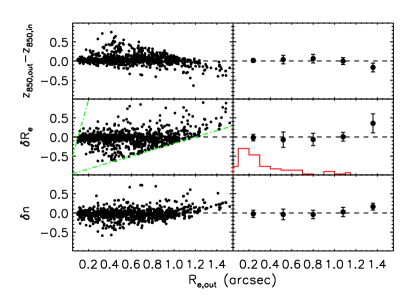
Figure 1.— Robustness of the fitting method: comparison of the estimated and input parameters (magnitude: $(z_{850,out}-z_{850,in})$, effective radius: $\delta R_{e}=(R_{e,out}-R_{e,in})/R_{e,in}$, Sérsic index: $\delta n=(n_{out}-n_{in})/n_{in}$) versus the input effective radius $R_{e,in}$ (left panel) and the measured effective radius $R_{e,out}$ (right panel). In the right part of each panel, we bin the values with x-axis value bins: the plots show the mean value and the scatter for each bin. The red histogram in the right panel represents in arbitrary units the $R_{e}$ distribution for our real ETGs. The green dashed lines delimit the possible $\delta R_{e}$ values due to the range of the simulation input values of $R_{e,in}$: because of the definition of $\delta R_{e}$ and of $0.1\arcsec\leq R_{e,in}\leq 1.2\arcsec$, a galaxy with $R_{e,out}$ will necessary have a corresponding value of $\delta R_{e}$ within [$R_{e,out}/1.2\arcsec-1$,$R_{e,out}/0.1\arcsec-1$]. For $0\arcsec\leq R_{e,out}<1.2\arcsec$, the size range spanned by our sample (see the text for more details), there are no significant systematics in the $R_{e}$ and $n$ parameters. Using the maximum scatter for binned simulated data, we assign an error of 20% to our measured $R_{e}$ and $n$.

When looking at $\delta R_{e}$ as a function of $R_{e,in}$ (left panel), we observe that our method recovers the effective radius with no significant bias, except for large galaxies ($R_{e,in}\gtrsim 1$″), where it slightly underestimates (by $\sim 5\%$) the radius, because a significant part of the light is lost in the background noise. When looking at $\delta R_{e}$ as a function of $R_{e,out}$ (left panel), we again observe no significant bias except for the galaxies with $R_{e,out}\geq 1.2$″, which have their size overestimated. This is a direct consequence of the chosen range for $R_{e,in}$ ([0.1″,1.2″]): as the green dashed line illustrates, all our simulated galaxies with $R_{e,out}\geq 1.2$″  can only have their size overestimated. Our real ETGs never have values of derived $R_{e}$ so high, as shown in the red histogram. These correlations propagate to magnitudes and Sérsic indexes.

In the range of our data ($0\arcsec\leq R_{e,out}<1.2\arcsec$), sizes and Sérsic indexes are recovered with systematics smaller than 8% and the magnitudes with systematics smaller than 0.08 mag, and also with a relatively small scatter. Hence our estimates of magnitude, $R_{e}$ and $n$ are well recovered, in the range covered by our observations. Using the maximum scatter for binned simulated data, we assign an error of 20% to our measured $R_{e}$ and $n$.

3.3. de Vaucouleurs vs Sérsic profile

To reduce uncertainties in the fit, we tried reducing the number of free parameters by using a fixed de Vaucouleurs (1948) profile ($n=4$). We estimated how such a fit would be reliable as compared to a Sérsic profile. We perform our fits again (real ETGs and simulations) with the same method, but this time with a de Vaucouleurs profile. We then compare the results with those obtained with a Sérsic profile ($n$ free) in Figure 2. The left panel represents $z_{850,out}^{n=4}-z_{850,out}$ and the right panel log($r_{e,out}^{n=4}/r_{e,out}$) as a function of the output Sérsic index $n_{out}$. Real ETGs are represented with large symbols (Lynx cluster: red dots, Lynx group: blue triangles, CDF-S: green stars) and simulations with black dots. ETGs with non robust structural parameter estimates are plotted as empty symbols. Real ETGs measurements and simulations show the same trend: measuring the size by assuming a de Vaucouleurs profile introduces a significant bias, which depends on the Sérsic index of the ETG. Those results are in qualitative agreement with those of D’Onofrio et al. (2008) and Taylor et al. (2010). We will use size and $n$ estimates obtained with a Sérsic profile hereafter. The tables in Appendix A present sizes and surface brightnesses derived with both Sérsic and de Vaucouleurs profiles. We present in Figure 10 in Appendix B the Sérsic index distributions for our sample. We remark that the presence of few ETGs with small Sérsic indexes is not unexpected, as they have been visually selected through their morphology.

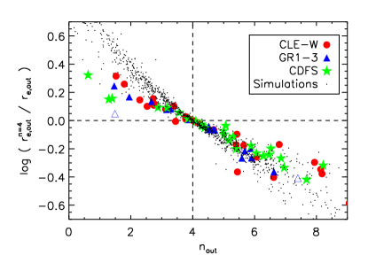
Figure 2.— Comparison of the estimated $z_{850}$ magnitude (left panel) and the estimated $R_{e}$ (right panel) when using a de Vaucouleurs profile (n=4) or a Sérsic profile (n free): real ETGs are represented with large symbols (Lynx cluster: red dots, Lynx group: blue triangles, CDF-S: green stars) and simulations with black dots. ETGs with non robust structural parameter estimates are plotted as empty symbols. For both magnitude and $R_{e}$, we observe a systematic bias depending on the Sérsic index $n$.

4. Kormendy relation (KR)

A powerful tool to investigate the ETG evolution and constrain the underlying processes is the Fundamental Plane (Djorgovski & Davis 1987; Dressler et al. 1987), which is a scaling relation between the effective radius $R_{e}$, the mean surface brightness $\langle\mu\rangle_{e}$ and the central velocity dispersion $\sigma_{0}$. As obtaining velocity dispersions of ETG at z $\sim$ 1 is observationally expensive, many studies have focused on the projection of the Fundamental Plane along the velocity dispersion axis, known as the Kormendy Relation (KR) (Kormendy 1977):

$$\langle\mu\rangle_{e}=\alpha+\beta\times log\>R_{e},$$ (3)

where $R_{e}$ is in kpc. The value of $\alpha$ depends on the photometric band and on the redshift. The slope $\beta$ has been found to be constant out to z = 0.64 (La Barbera et al. 2003).

We convert our $z_{850}$ magnitudes in the $B$–band rest–frame, $B_{z_{0}}$, in order to derive the $B$–band rest-frame surface brightness $\langle\mu^{B}\rangle_{e}$. We use the index $z_{0}$ to refer to the rest-frame and $z_{obs}$ to refer to the observed frame. To estimate $B_{z_{0}}$, we use a method similar to the one used in Mei et al. (2009). We use CB07 models (choosing BC03/MA05 models changes $B_{z_{0}}$ by less than 0.1 mag) and consider a set of galaxies with a redshift of formation $1.8\leq z_{form}\leq 7$, a solar metallicity and an exponentially declining SFH with $0.1\leq$ SFH $\tau$ (Gyr) $\leq 1$. We then linearly fit the relation between the colors ($B_{z_{0}}-z_{850,z_{obs}}$) and ($i_{775,z_{obs}}-z_{850,z_{obs}}$) (where $i_{775,z_{obs}}$ and $z_{850,z_{obs}}$ are the apparent magnitudes in the $i_{775}$ and $z_{850}$ bands for galaxies observed at $z=z_{obs}$). Once this relation is established, we can estimate the total $B$–band rest-frame magnitude $B_{z_{0}}$ from the full measured apparent magnitude in the $i_{775}$ and $z_{850}$ bands (published in R11). Eventually, we transform this magnitude into mean surface brightness by averaging half of the total flux on the surface within $R_{e}$ and correct for the cosmological dimming $(1+z_{obs})^{4}$:

$$\langle\mu^{B}\rangle_{e}=B_{z_{0}}+2.5\times log(2\pi R_{e}^{2})-10\times log(1+z_{obs}).$$ (4)

Taking into account the different steps in estimating $\langle\mu^{B}\rangle_{e}$, we assign an uncertainty of 0.4 mag for our $\langle\mu^{B}\rangle_{e}$ estimate.

The KR we obtain is plotted in Figure 3. The upper panels show our KR for the three environments: Lynx cluster ETGs (left panel a), red dots), Lynx group ETGs (middle panel b), blue triangles) and CDF-S field ETGs (right panel c), green stars). ETGs with non robust structural parameter estimates are plotted as empty symbols. For each environment, the colored area represents the 1$\sigma$ dispersion of the best linear fit to our data, done through a classical chi-square error statistic minimization. The red dotted line represents a line of constant absolute magnitude $M^{B}_{z_{0}}=-20.2$ mag, corresponding to our cut in selection at $z_{850}=24$ mag. The black solid and dashed lines represent the local KR: they represent the best linear fit and its 1$\sigma$ dispersion to the data measured in the $B$–band by Jorgensen et al. (1995) for 31 ETGs in the Coma cluster (converted to the AB magnitude system). As Jorgensen et al. (1995) sizes are estimated with a de Vaucouleurs profile and we have demonstrated that this changes the size estimate (Figure 2), we use an approach similar to La Barbera et al. (2003) and exclude from this sample the three largest galaxies (log($R_{e}$/kpc) $\gtrsim 1$) for which the size difference between a de Vaucouleurs and a Sersic profile is likely to be significant. In order to show that this choice of local relation does not affect our conclusions on the KR, we display in Figure 11 in Appendix B a figure similar to Figure 3, but with our sizes estimated with a de Vaucouleurs profile instead of a Sérsic profile and with including in Jorgensen et al. (1995) local relation the three largest galaxies.

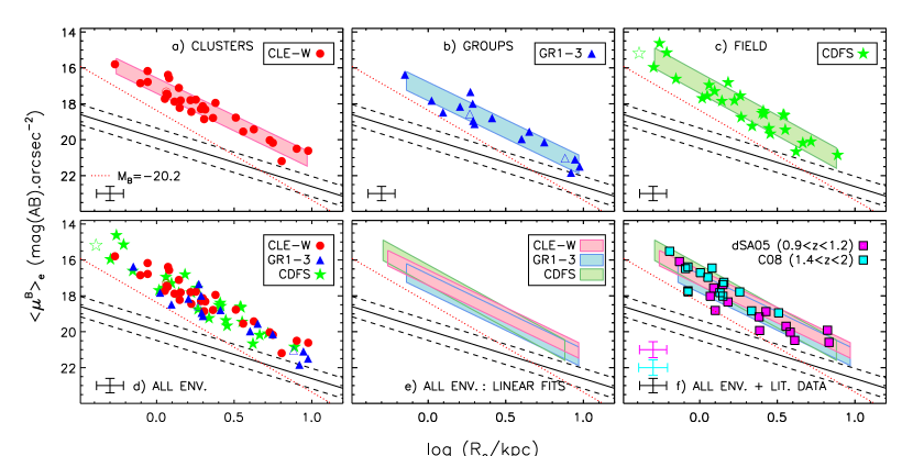
Figure 3.— Upper panels a), b), c): Kormendy relation for our ETGs at $z\sim 1.3$ in rest-frame $B$–band. Lynx cluster ETGs (a), red dots), Lynx group ETGs (b), blue triangles) and CDF-S ETGs (c), green stars). ETGs with non robust structural parameter estimates are plotted as empty symbols. For each environment, the colored area represent the 1$\sigma$ dispersion of the best linear fit to our data. Typical uncertainties are represented by the cross in the lower left corner. The black solid and dashed lines represent the local KR (Jorgensen et al. 1995) and the 1$\sigma$ dispersion for the Coma cluster, respectively. The red dotted line represents a line of constant absolute magnitude $M^{B}_{z_{0}}=-20.2$ mag, corresponding to our cut in selection at $z_{850}=24$ mag. Lower panels d), e), f): Kormendy relation for the three environments simultaneously. In (d) we show our data and in (e) the areas corresponding to the 1$\sigma$ scatter of a linear fit. In (f): same as panel e), but with data from the literature; dSA05 corresponds to the sample of di Serego Alighieri et al. (2005) and C08 corresponds to the sample of Cimatti et al. (2008) (see text). Our Kormendy relation does not depend on the environment and is in qualitative agreement with passive evolution when comparing with $z\sim 0$ and $z\sim 1$-2 literature data.

4.1. KR: dependence on the environment

As shown in previous works at $z>1$, the KR is in place at $z\sim 1.3$ in the field (e.g., di Serego Alighieri et al. 2005; Longhetti et al. 2007; Cimatti et al. 2008; Damjanov et al. 2009; Saracco et al. 2009) and in clusters (e.g., Holden et al. 2005; Rettura et al. 2010). We find that, though the range in size is similar for the three environments, the distribution of cluster ETGs seems to be more concentrated towards smaller sizes. We will come back to this point in $\S$5. We then plot the data for our whole sample in the lower left panel d) and the 1$\sigma$ dispersion around the best linear fit relations in the lower middle panel e). The KRs in the three environments are in agreement, and we do not observe any dependence of the KR on the environment at $z\sim 1.3$. Rettura et al. (2010) studied the KR in the field and in a cluster at $z\sim 1.2$ and found no dependence on the environment. Our work confirms this study and extends its results to the group environment.

4.2. KR: comparison with the local relation

When comparing with the local KR, we observe that our relation is shifted towards brighter luminosities and the slope is steeper. This change in slope may be linked to the magnitude cut due to the depth of our $z_{850}$ image (see the line showing the depth of our ACS image in Figure 3), or be a real steepening of the KR.

Stellar population models predict that the luminosity evolution depends on galaxy age and its SFH. In Figure 4, we show these dependences between $z\sim 1.26$ and $z=0$. We plot the luminosity evolution as a function of age at the given redshift for several exponentially declining SFHs with characteristic time SFH $\tau$ ranging from 0.1 to 1 Gyr. The range in SFH $\tau$ encompasses the likely values for our ETGs: for all models (BC03/MA05/CB07), our estimated maximum SFH $\tau$ is below 1 Gyr for 90% of our sample (R11; see also Rettura et al. 2011). If evolving passively down to $z=0$, a 3 Gyr old ETG at $z=1.26$ will be 1.5-2.5 mag less luminous in $B_{z_{0}}$ whereas a 1 Gyr old ETG at $z=1.26$ will be 3-3.5 mag less luminous in $B_{z_{0}}$. Older ETGs evolve less in $B_{z_{0}}$.

In Figure 5, we code our galaxy ages (as derived from R11, see this paper for details) in gray levels, for the three models (BC03/MA05/CB07). Larger ETGs tend to be older. To better visualize this trend, we bin our data in three size bins (log($R_{e}$/kpc) $<$ 0, 0 $\leq$ log($R_{e}$/kpc) $<$ 0.5 and log($R_{e}$/kpc) $\geq 0.5$). For each size bin, we overplot as magenta squares the mean and the 1$\sigma$ dispersion for log($R_{e}$/kpc) and $\langle\mu^{B}\rangle_{e}$ values. We report, in orange at the bottom of the figure, the mean and standard deviation of the estimated ages for each bin. Thus, we observe an age gradient in our KR, larger ETGs being on average older, because they are on average more massive (see also R11; such an age gradient is observed in the local Universe, see for instance Shankar et al. 2010). Under the assumption of only passive evolution in luminosity and according to stellar population models, this age gradient should lead to a steepening of the slope of the KR with increasing redshift, in qualitative agreement with what we observe.

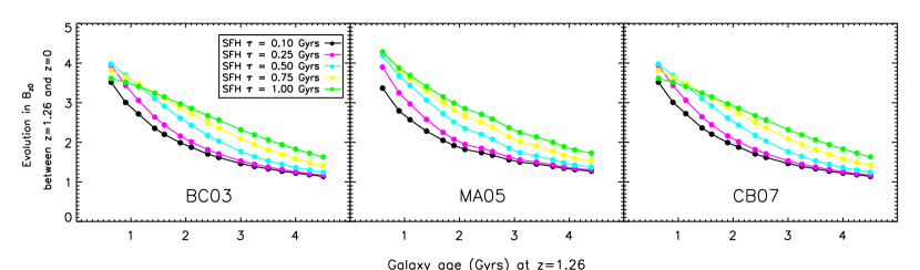
Figure 4.— Theoretical luminosity evolution in rest-frame $B_{z_{0}}$ magnitude: for different SFH $\tau$, we plot the difference $B_{z_{0}}$($z$=1.26) - B${}_{z_{0}}$($z$=$z_{0}$) predicted by the three stellar population models as a function of the age of the ETG at $z=1.26$. Older ETGs at $z=1.26$ evolve less in $B_{z_{0}}$.

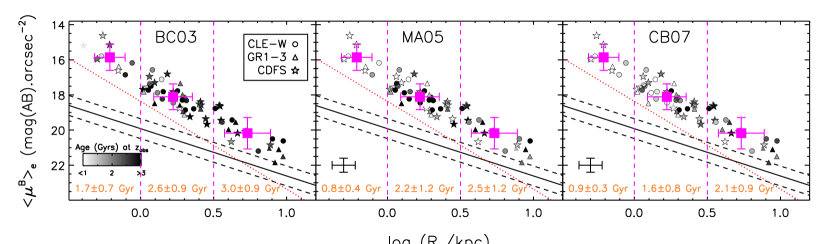
Figure 5.— Kormendy relation at $z\sim 1.3$: dependence on age. Our KR is plotted with ages estimated from three models (BC03/MA05/CB07) which are coded in gray levels. ETGs with non robust structural parameter estimates are plotted without black outlines. The solid and dashed black lines and the red dotted lines are the same as in Figure 3. We bin our data in three size bins (vertical dashed magenta lines): for each bin, we overplot as magenta squares the mean and the 1$\sigma$ dispersion for log($R_{e}$/kpc) and $\langle\mu^{B}\rangle_{e}$ values. We also report, in orange at the bottom of the figure, the mean and standard deviation of the estimated ages for each bin. On average, large ETGs are older than smaller ones.

4.3. KR: comparison with literature data at $z\sim 1$-2

On the panel f) of Figure 3, we overplot as squares with black outlines the KRs published for ETGs at $z_{spec}\sim 1$-2 . The sample from di Serego Alighieri et al. (2005) (in magenta) is composed of 16 field ETGs (from the K20 survey, selected according to their spectra) at $0.9\leq z_{spec}\leq 1.2$ (we removed the two ETGs at $z_{spec}\sim 0.67$). The size is estimated by using Gim2d (Simard et al. 2002) and fitting a Sérsic profile on HST/ACS $z_{850}$-band and VLT/FORS-1 $z$-band images. The sample from Cimatti et al. (2008) (in light blue) is composed of 13 passive galaxies (6 in the field and 7 in a cluster-like structure) selected from the GMASS project, mainly ETGs, with $1.4\leq z_{spec}\leq 2$. The size is estimated using Galfit by fitting Sérsic profiles to HST/ACS $z_{850}$-band images. For those two samples, the radius is the circularized effective radius. We converted the surface brightness to the AB magnitude system for the sample of di Serego Alighieri et al. (2005).

From this comparison, we can observe two facts. Firstly, we observe that our KR is broadly consistent with those two studies. The KR from di Serego Alighieri et al. (2005), observed at lower redshifts, is slightly shifted towards fainter luminosities and the KR from Cimatti et al. (2008), observed at higher redshifts, is lying on the higher luminosity side of our KR. Thus, putting together those three KRs, we see a shift of the KR towards bright luminosities with increasing redshift, qualitatively consistent with passive luminosity evolution.

Secondly, looking at the range in size, we notice that the sample of di Serego Alighieri et al. (2005) lacks galaxies smaller than 1 kpc, even if comparable to our sample in a $K_{s}$-band limit magnitude, and is comparable to our sample for large galaxies. The sample of Cimatti et al. (2008) lacks galaxies larger than $\sim$3 kpc and is comparable to our sample for small sizes. We remark that the observed lack of small/large galaxies in those two samples is not a selection effect due to the depth of the images, which would produce a cut along a line parallel to the red dotted line (di Serego Alighieri et al. (2005) limiting magnitude is about $M^{B}_{z_{0}}=-20.1$ mag and Cimatti et al. (2008) data are deep enough to detect a galaxy at $M^{B}_{z_{0}}=-20.2$ mag). Our sample ranges a larger interval in size that both other samples.

5. Mass-size relation (MSR)

In Figure 6, we plot our MSR, derived using the three stellar population models (BC03/MA05/CB07), and splitting our sample by environment: we display from upper to lower panels, Lynx cluster ETGs (red dots), Lynx group ETGs (blue triangles), CDF-S ETGs (green stars) and all environments simultaneously. The solid and dashed lines represent the local MSR scaled to a Salpeter IMF, and its 1$\sigma$ relation, respectively. The local MSR established by Shen et al. (2003) with sizes estimated in $z$ band for SDSS galaxies selected according to their Sérsic index ($n\geq 2.5$) is in cyan. The local MSR established by Valentinuzzi et al. (2010a) with sizes estimated in $V$ band for WINGS cluster galaxies that were morphologically selected to be ETGs is in magenta. The difference in the rest-frame used to estimate sizes would shift the local MSRs towards larger sizes (around 10%-15% according to Bernardi et al. 2003). We compare our sample with Valentinuzzi et al. (2010a), because both select ETGs from a morphologically classification. All our results do not change when using Shen et al. (2003) local MSR, which is widely used in the literature.

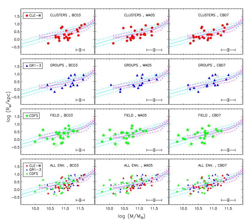
Figure 6.— Mass-size relation at $z\sim 1.3$ derived with the three stellar population models (BC03/MA05/CB07), split by environments: from upper to lower panels, Lynx cluster ETGs (red dots), Lynx group ETGs (blue triangles), CDF-S ETGs (green stars) and all environments simultaneously. ETGs with non robust structural parameter estimates are plotted as empty symbols. Magenta (resp. cyan) solid and dashed lines represent the local relation of Valentinuzzi et al. (2010a) (resp. Shen et al. 2003) and its 1$\sigma$ dispersion. Typical uncertainties are represented by the cross in the right left corner. When quantifying size evolution, one has to be careful to the model and local MSR used (see Table 1). Most of cluster and group ETGs lie below local MSRs, whereas field ETGs are in agreement with local MSRs (except with BC03 models, for which more field ETG lie below the local MSRs, see text for discussion).

5.1. MSR: dependence on the environment

We plot in Figure 7, for the three environments and the three models, the normalized distributions of the size ratio $R_{e}/R_{e,Valen.}$, which represents the ratio between the size of our ETGs and the one predicted by the local MSR of Valentinuzzi et al. (2010a) at similar masses. For each histogram, we overplot with a black solid line the best-fit gaussian to the distribution, obtained through a non-linear least-squares fit. As found in previous studies at $z\sim 1$-2, our sample presents a significant number of ETGs having small radii compared to the local ones of similar mass. However, the precise number of such ETGs and the value of size ratios depend on the model (and the local MSR used as a reference). We display in Table 1 the mean and standard deviation corresponding to the gaussian fit. For qualitative comparison, we also display in this Table the corresponding values when comparing our sizes to Shen et al. (2003) local MSR.

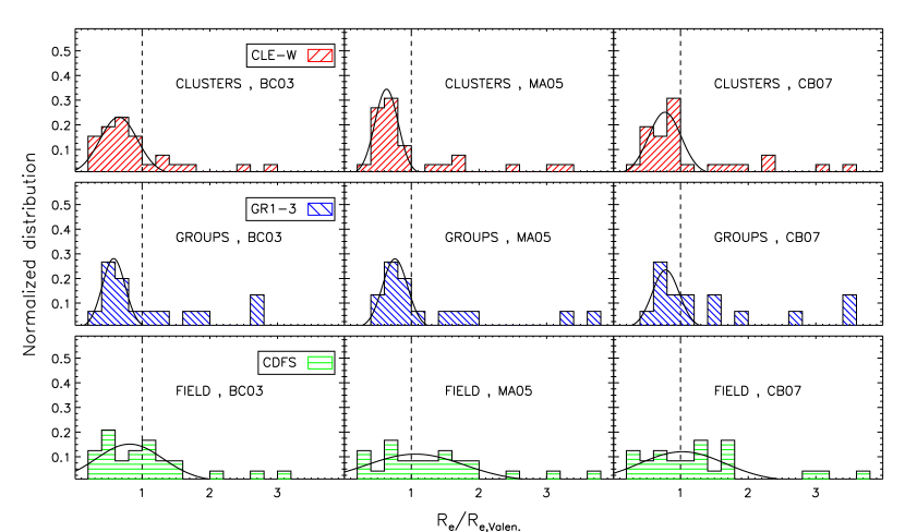
Figure 7.— Size ratio $R_{e}/R_{e,Valen}$ normalized distributions derived with the three stellar population models (BC03/MA05/CB07), split by environments: Lynx cluster ETGs (upper panels, red tilted lines), Lynx group ETGs (middle panels, blue tilted lines) and CDF-S ETGs (lower panels, green horizontal lines). $R_{e}/R_{e,Valen}$ represents the ratio between the size of our ETGs and the one predicted by the local MSR of Valentinuzzi et al. (2010a). The black solid line represents the best-fit gaussian to the distributions. The black dashed line represents the locus of $R_{e}/R_{e,Valen}=1$. For MA05/CB07 models, field ETG population is in agreement with the local MSR, whereas cluster/group ETG population lie below the local MSR.

Table 1Size Ratios as a Function of Stellar Population Model, Local MSR, and Environment

Environment	$R_{e}/R_{e,Valen}$			$R_{e}/R_{e,Shen.}$
	BC03	MA05	CB07	BC03	MA05	CB07
CLE-W	0.7 $\pm$ 0.3	0.6 $\pm$ 0.2	0.8 $\pm$ 0.2	0.5 $\pm$ 0.2	0.5 $\pm$ 0.1	0.7 $\pm$ 0.2
GR1-3	0.6 $\pm$ 0.2	0.8 $\pm$ 0.2	0.8 $\pm$ 0.2	0.6 $\pm$ 0.2	0.7 $\pm$ 0.2	0.8 $\pm$ 0.2
CDF-S	0.8 $\pm$ 0.5	1.1 $\pm$ 0.7	1.0 $\pm$ 0.6	0.7 $\pm$ 0.3	1.1 $\pm$ 0.6	1.0 $\pm$ 0.5
All	0.7 $\pm$ 0.4	0.7 $\pm$ 0.2	0.8 $\pm$ 0.4	0.6 $\pm$ 0.3	0.6 $\pm$ 0.2	0.8 $\pm$ 0.3

Despite the dependence on the model (and on the local MSR), there is a general trend : most of the cluster and group ETGs lie below local MSRs. We observe in Figure 7 that cluster and group ETG size ratios are mostly below 1 with a narrow distribution that peaks around 0.6-0.8, whereas field ETG size ratios have a more widespread distribution, peaking around 0.7-1.1. The values in Table 1 confirm this point, i.e. that at a given mass, ETGs in denser environments tend to have smaller sizes at $z\sim 1.3$ than in the local Universe. From a Kolmogorov-Smirnov (Kuiper) statistical test, the cluster and field samples for ETGs with masses $M<10^{11}M_{\sun}$ do not have the same size ratio distributions, at 85% (90%) and 90% (95%) using MA05 and CB07 models, respectively. Using BC03 stellar population models, on the other hand, the null hypothesis (the cluster and field samples are taken from the same statistical distribution) cannot be rejected (rejected at only 40% and 60% confidence for a Kolmogorov-Smirnov and Kuiper test, respectively), in this mass range, and it is rejected at 86% and 90%, respectively, on the entire mass range. We underline that the Kuiper test is more sensitive to the shape of the distribution than the Kolmogorov-Smirnov test.

We remark that our size ratios in clusters are in agreement with previous estimates in high redshift clusters (Rettura et al. 2010; Strazzullo et al. 2010). We know that ETGs with emission lines have higher size ratios (e.g. Toft et al. 2007; Zirm et al. 2007; Williams et al. 2010). Even when we remove them (Salimbeni et al. 2009; Holden, Nakata, private communication) our distributions remain similar as in Figure 7, as it can be seen in Figure 12 in Appendix B.

The field ETG population is approximately equally divided with ETGs above and below the local MSRs, except when using the BC03 models, in which case a majority lie below the local MSRs. This can be explained by the underestimate of the TP-AGB phase by BC03 models. As explained in previous works (e.g. Maraston et al. 2006; Conroy & Gunn 2010; R11), this underestimate leads to an artificial increase of the estimated age and mass of galaxies with ages $\sim$1-2 Gyr (see Figure 5 & 6 of R11). Such an ETG will be estimated with an older age and a greater mass: it will be shifted towards the more massive area in Figure 6 and thus will more likely lie below the local MSRs. This effect of BC03 models is more obvious for our CDF-S sample, because this sample contains more ETGs with ages $\sim$1-2 Gyr (see R11).

In R11, we underlined that our CDF-S sample might be biased against low-mass/passive ETGs, because their low luminosity and the lack of emission line prevent to derive reliable spectroscopic redshift. We have tested that our conclusions for the field sample do not depend on this potential bias. We have selected a new sample of GOODS/CDF-S ETGs, using photometric redshifts from Santini et al. (2009) and we obtain a MSR that again shows a distribution similar to the local. The selection criteria are described in Appendix B and the results are in Figure 13.

If on the other hand, we are missing massive galaxies, this would not change the overall mass-size distribution, which clearly shows to be similar to the local one at all masses and will not be changed significantly by rare massive galaxies.

5.2. Size ratio versus redshift of formation/stellar mass

We now check the dependence of the size ratio on the redshift of formation. We plot in Figure 8 the size ratio $R_{e}/R_{e,Valen.}$ as a function of the redshift of formation $z_{form}$. For indication, we also mark with thick black outline the ETGs known to have emission lines and with a thick orange outline the ETGs known to be passive (Salimbeni et al. 2009; Holden, Nakata, private communication). As already observed in the literature (e.g. Valentinuzzi et al. 2010a; Williams et al. 2010), when looking at our results with MA05/CB07 models, we observe that passive/quiescent ETGs tend to have small size ratios, whereas line-emitting/star-forming ETGs tend to have larger size ratios.

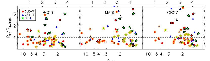
Figure 8.— Size ratio versus redshift of formation, derived with the three stellar population models (BC03/MA05/CB07): Lynx cluster ETGs are red disks, Lynx group ETGs are blue triangles and CDF-S ETGs are green stars. ETGs with non robust structural parameter estimates are plotted as empty symbols. We also mark with thick black outline the ETGs known to have emission lines and with thick orange outline the ETGs known to be passive. The black dashed line represents the locus of $R_{e}/R_{e,Valen}=1$. For MA05/CB07 models and cluster/group environments, ETGs with small size ratios have equally distributed $z_{form}$ and ETGs with high size ratios are younger ETGs ($z_{form}\lesssim 3$). For the field, our sample do not show old galaxies (see also R11) probably because it does not cover large areas. However, again, field galaxies cover a larger distribution in sizes.

If we consider the plots with MA05/CB07 models (for which the redshift of formation is more robust because of the better modeling of the TP-AGB stellar phase), most of cluster and group ETGS lie below the local MSRs, as already shown in Section 5.1. We also observe that galaxies with small size ratios do not have a preferred redshift of formation and, on the other hand, there is a deficit of ETGs with $z_{form}\gtrsim 3$ and a high size ratio ($R_{e}/R_{e,Valen.}\gtrsim 2$).

Figure 9 shows the dependence of the size ratio on the stellar mass. We do not observe any clear dependence of the size ratio on the stellar mass. In particular, for MA05/CB07 models and all environments, ETGs with small size ratio span the whole range in mass of our sample. Moreover, the high-mass end of our sample ($M\gtrsim 2\times 10^{11}M_{\sun}$, see also Figure 6) is in agreement with the local MSR for all environments.

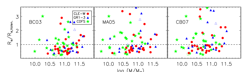
Figure 9.— Size ratio versus stellar mass, derived with the three stellar population models (BC03/MA05/CB07): symbols are as in Figure 8. We do not observe any clear dependence of the size ration on the stellar mass.

5.3. MSR: comparison with literature data at $z\sim 1$-2

Our results are consistent with published works of the MSR at the same redshift and with comparable mass range, i.e. $10^{10}\lesssim M/M_{\sun}\lesssim 3\times 10^{11}$.

Valentinuzzi et al. (2010b), whose sample covers masses slightly higher to those of this work up to a redshift $z\sim 0.7$, have found that the median MSR in galaxy clusters have only mildly evolved between $z\sim 0.7$ to the present (size ratio $\sim 0.5$-0.8 when comparing ETG populations). Working with a Kroupa (2001) IMF and on a mass-selected sample ($M_{Kroupa}\geq 4\times 10^{10}M_{\sun}$), and defining a superdense galaxy as a galaxy with $\Sigma_{50}=\frac{0.5\times M_{Kroupa}}{\pi R_{e}^{2}}\geq 3\times 10^{9}M_{\sun}$ kpc^-2, these authors find that 41% of their $z\sim 0.7$ cluster sample is made of superdense galaxies, against 17% for $z\sim 0$ cluster sample (Valentinuzzi et al. 2010a). Using the very same criteria, we find that $\sim 45\%$ (BC03) or $\sim 35\%$ (MA05/CB07) of our cluster sample is made of superdense galaxies. The mass cut reduces our cluster sample to $\sim$ 15 galaxies, lowering the statistics: assuming Poissonian errors on our number of galaxies leads to an uncertainty of $\sim 20\%$ on our estimated percentages. A correct estimate should also take into account the different galaxy selection and size estimate methods.

Newman et al. (2010) study a sample of field spheroidals with masses $6\times 10^{10}<M/M_{\sun}<3\times 10^{11}$ in the redshift range $1.1<z_{spec}<1.6$. They find that galaxies less massive than $10^{11}M_{\sun}$ lie on the local MSR, and those more massive than $10^{11}M_{\sun}$ have to grow of around twice in size. Those results are consistent with our founding in the field.

Saracco et al. (2011) study field and cluster (among which Lynx members) ETGs lying at $0.9<z_{spec}<2$. They find that compact ETGs formed over a wide range of redshift ($2<z_{form}<10$) and that normal ETGs have formed at $z\lesssim 3$. Our results are in agreement, since we find that our cluster ETGs (more compact) formed over a wide range of redshifts and field ETGs (that have younger ages) have a larger dispersion in sizes. In our sample these different distributions seems to be linked to the environment. They also find compact ETGs throughout all their probed mass range ($5\times 10^{10}<M/M_{\sun}<5\times 10^{11}$).

van der Wel et al. (2008) studied a sample of morphologically selected ETGs in field and cluster environments at $0.8<z_{spec}<1.2$ and, using dynamical masses, found that ETGs have on average increase their size by a factor of 2 between $z\sim 0$ and $z\sim 1$. This result is at apparent discrepancy with ours for field ETGs. However, these two works probe different ranges in galaxy mass: our sample spans masses of $10^{10}<M/M_{\sun}<3\times 10^{11}$, whereas van der Wel et al. (2008) sample includes more massive, $8\times 10^{10}<M/M_{\sun}<10^{12}$ (when dynamical masses are converted to Salpeter stellar masses). In addition, van der Wel et al. (2008) sizes are estimated using de Vaucouleurs profile, which complicates a possible comparison for the few ETGs in common with similar mass (see §.3.3 and Figure 2). The fact that van der Wel et al. (2008) do not find an environmental dependence on the evolution of the MSR and we do, probably reflects the different range in mass probed by the two works. This points to a very interesting situation since it suggests that the evolution of the MSR is mass dependent.

Recent works have found very compact galaxies in the field at $z_{spec}\gtrsim 1.5$ (e.g. Daddi et al. 2005; van Dokkum et al. 2008; Damjanov et al. 2009; van Dokkum et al. 2010). The mass range covered in these works ($M\gtrsim 2\times 10^{11}M_{\sun}$, when converted to Salpeter stellar masses) hardly overlaps our mass range, and we thus cannot compare conclusions directly because we are sampling different ranges in mass and in redshift.

Our results are driven by galaxies with masses $M\lesssim 2\times 10^{11}M_{\sun}$. Our galaxies with masses $M\sim 10^{11}M_{\sun}$ follow the same trends that the entire sample: field galaxies lie on the local MSR relation, cluster galaxies show an average MSR shifted to sizes 30-50% smaller. Our galaxies with masses $M\gtrsim 2\times 10^{11}M_{\sun}$ are a few, and show a large dispersion in size: they lie on the local MSR independently of the environment (see Figure 6), but their small number does not permit us to draw conclusions on their behaviour.

6. Conclusions

In this work, we have studied a sample of 76 ETGs spanning a wide range of environments (cluster, group, and field) at $z\sim 1.3$, combining multi–wavelength observations of the Lynx supercluster, with data on the GOODS/CDF-S field. We estimated the size of our ETGs by fitting a Sérsic profile to the HST/ACS $z_{850}$ images, which probe the rest-frame $B$-band. Combining those sizes with stellar masses and stellar population ages derived in R11, we are able to study two crucial structural relations, the Kormendy relation and the mass-size relation, in three different environments at $z\sim 1.3$.

We obtain the following results:

1. The Kormendy relation, in place at $z\sim 1.3$, does not depend on the environment. We thus confirm the result of Rettura et al. (2010) and extend it to the group environment. Our results are in agreement with results in the cluster and field samples of di Serego Alighieri et al. (2005) and Cimatti et al. (2008).

2. Concerning the mass-size relation, for all stellar population models (BC03/MA05/CB07) and local relations (Shen et al. 2003; Valentinuzzi et al. 2010a), ETGs are on average more compact in denser environments. When comparing the MSR at high redshift with the one in the local universe, the uncertainty on the mass coming from the model used to estimate it and the choice of the local MSR can significantly influence the conclusion on the importance of the size evolution. When using MA05/CB07 models, we find that the majority of cluster and group ETGs are below the local relations, whereas field ETGs follow a MSR similar to the local one. From a Kolmogorov-Smirnov (Kuiper) statistical test, the cluster and field samples for galaxies with masses $M<10^{11}M_{\sun}$ do not follow the same size ratio distribution, at 85% (90%) and 90% (95%) using MA05 and CB07 models, respectively. When using BC03 models, the two distributions do not differ.

3. When using MA05/CB07 models, we find that compact ETGs do not have a preferred redshift of formation. Those results are in close agreement with those of Saracco et al. (2011), who studied a sample of 62 ETGs with $0.9<z_{spec}<2$. As concluded by these authors, the lack of dependence of the compactness on the redshift of formation is not consistent with models that predict compact galaxies to have formed at earlier times, when the Universe was more dense.

When we compare the MSR of cluster and group ETGs vs field ETGs, we find that, at similar masses, cluster and group ETGs are more compact than field ETGs. On average this does not depend on cluster galaxy age. This result is in contrast with what has been found so far for field galaxies at $z\sim 1$ at higher masses (e.g. van der Wel et al. 2008), and it might be due to the different range in masses that we are probing. If this was confirmed by larger samples, it would mean that environmental effects are visible in the evolution of the MSR for ETGs with $M\lesssim 2\times 10^{11}M_{\sun}$.

Our results are mainly driven by galaxies with masses $M\lesssim 2\times 10^{11}M_{\sun}$. Our galaxies with masses $M\sim 10^{11}M_{\sun}$ follow the same trends that the entire sample. Our galaxies with masses $M\gtrsim 2\times 10^{11}M_{\sun}$ are a few, but they lie on the local MSR independently of the environment (see Figure 6); however their small number does not permit us to draw conclusions on their behaviour. As concluded by other authors (Newman et al. 2010; Cassata et al. 2011; Saracco et al. 2011), the very compact galaxies at $z\sim 2$ should have gone a dramatic evolution in size to reproduce our results at $z\sim 1.3$. This growth between $z\sim 2$ and $z\sim 1$ seems to be somehow different in cluster and field galaxies. Cassata et al. (2011) have shown that, in the field, ETGs enlarge their size and increase their stellar mass by a factor of 5 between $z=2$ and $z\sim 1$. At $z\sim 1.3$, field galaxies are already on the local MSR, while cluster galaxies still have compact sizes on average (see also Strazzullo et al. 2010; for a similar result at $z=1.4$), indicating that their size distribution still needs to be enlarged (see also Valentinuzzi et al. 2010b).

Since in the local Universe, the ETG MSR does not depend on environment (Maltby et al. 2010), our results imply that an evolution in the MSR of cluster and group ETG size is required to explain current observations, while field ETGs show a MSR that is compatible with the local one. The evolution of the MSR in dense environments might reflect either an evolution in size of the pristine population or the transformation of ETG progenitors that are not classified as ETG at $z\sim 1.3$ or the accretion of a new population of larger ETGs.

In the first case, minor dry merger events could have enlarged the size of the ETG population. In the second case, compact ETGs might have not had much evolution, but a new population of larger ETGs could have been formed by not-ETG progenitors or accreted in dense environments at $z<1$ (Valentinuzzi et al. 2010b). This new population might not have been observed at $z\sim 1.3$ because its progenitors are not ETGs at that time. These galaxies might be disk galaxies that have evolved from a large bulge spiral population or galaxy mergers (e.g., Postman et al. 2005; Mei et al. 2006a; Poggianti et al. 2006; Valentinuzzi et al. 2010b; Mei et al. 2011). For instance, according to semi-analytic models, the ETG population at $z\sim 1$ in dense environments contain less than $\sim 70\%$ of the stellar mass which ends up in ETGs at $z\sim 0$ (Kaviraj et al. 2009).

On the other hand, these results pose some challenges to current state-of-the-art galaxy evolution models that predict a nearly mass-independent size for ETGs (e.g. Shankar et al. 2011) and, we have checked, nearly independent of environment. More detailed theoretical work is required to fully understand all the processes at work that can affect galaxy sizes. This is clearly beyond the scope of the present work and will be the subject of future efforts.

Appendix A Appendix A: Lynx and CDF-S ETG structural parameters

Lynx (resp. CDF-S) ETG structural parameters are presented in Tables 2 and 3 (resp. Table 4)

Table 2Lynx cluster ETG structural parameters and surface brightness.

ID	R.A.	DEC.	$n$	$R_{e}$	$R_{e}$	$\langle\mu^{B}\rangle_{e}$
	(J2000)	(J2000)		(arcsec)	(kpc)	(AB mag.arcsec-2)
Lynx Cluster E ($\langle z\rangle=1.261$)
4945	08 48 49.99	+44 52 01.78	6.1	0.67	5.61	20.2
			4	0.37	3.12	18.9
6229	08 48 55.90	+44 51 54.99	9.1	0.77	6.40	21.2
			4	0.20	1.66	18.3
6090	08 48 56.64	+44 51 55.76	2.3	0.14	1.16	17.4
			4	0.19	1.63	18.2
5355	08 48 57.66	+44 53 48.69	5.4	0.16	1.30	17.9
			4	0.13	1.04	17.4
8713	08 48 57.85	+44 50 55.32	…	…	…	…
5817	08 48 57.91	+44 51 52.25	7.9	0.23	1.93	18.3
			4	0.12	0.98	16.8
5634	08 48 58.53	+44 51 33.25	3.8	0.51	4.23	19.4
			4	0.54	4.49	19.6
5693	08 48 58.60	+44 51 57.21	1.5	0.14	1.19	16.4
			4	0.28	2.36	17.9
5680	08 48 58.63	+44 51 59.46	1.8	0.20	1.65	17.8
			4	0.36	2.97	19.1
5794	08 48 58.67	+44 51 56.97	8.2	0.29	2.40	18.0
			4	0.12	0.96	16.0
8495	08 48 58.93	+44 50 33.77	3.4	0.10	0.88	16.8
			4	0.10	0.85	16.7
5748	08 48 58.95	+44 52 10.90	4.1	0.21	1.79	17.8
			4	0.21	1.74	17.7
5689	08 48 59.10	+44 52 04.64	4.2	0.20	1.67	18.4
			4	0.19	1.62	18.4
5876	08 48 59.72	+44 52 51.28	5.7	0.39	3.24	18.8
			4	0.26	2.18	17.9
5602	08 49 00.32	+44 52 14.39	4.7	0.24	1.98	18.1
			4	0.21	1.71	17.8
8662	08 49 01.07	+44 52 09.65	3.8	0.24	2.03	18.9
			4	0.26	2.14	19.0
8041	08 49 01.52	+44 50 49.73	2.7	0.17	1.39	17.1
			4	0.21	1.78	17.7
8625	08 49 03.31	+44 53 04.12	3.8	0.06	0.54	15.8
			4	0.07	0.55	15.8
7653	08 49 04.52	+44 50 16.42	3.9	0.09	0.79	16.9
			4	0.10	0.80	16.9
8047	08 49 05.34	+44 52 03.79	5.4	0.64	5.36	20.0
			4	0.43	3.62	19.2
7475	08 49 05.96	+44 50 37.00	4.0	0.10	0.88	16.2
			4	0.10	0.87	16.2
Lynx Cluster W ($\langle z\rangle=1.273$)
1745	08 48 29.71	+44 52 49.68	2.8	0.17	1.41	18.2
			4	0.21	1.79	18.8
1486	08 48 31.72	+44 54 42.95	6.8	0.14	1.13	17.7
			4	0.09	0.78	16.9
1794	08 48 32.78	+44 54 07.22	3.1	0.17	1.43	17.8
			4	0.21	1.72	18.2
1922	08 48 32.99	+44 53 46.69	2.5	0.14	1.20	16.6
			4	0.18	1.49	17.0
1525	08 48 33.01	+44 55 11.92	8.1	0.43	3.61	19.5
			4	0.20	1.65	17.8
1962	08 48 33.04	+44 53 39.75	5.4	0.14	1.18	17.5
			4	0.05	0.44	15.4
2094	08 48 34.08	+44 53 32.32	2.7	0.28	2.31	18.8
			4	0.39	3.26	19.5
2343	08 48 35.98	+44 53 36.12	3.4	1.13	9.47	20.6
			4	1.44	12.00	21.1
2195	08 48 36.17	+44 54 17.30	6.6	0.96	7.99	20.5
			4	0.38	3.19	18.5
2571	08 48 37.08	+44 53 34.05	4.0	0.25	2.06	18.3
			4	0.25	2.08	18.3

Note. — $R_{e}$ denotes the circularized effective radius. Uncertainties on $R_{e}$ are of 20%, uncertainties on $n$ are of 20% and uncertainties on $\langle\mu^{B}\rangle_{e}$ are of 0.4 magnitudes. We did not report parameters considered as non robust.

Table 3Lynx group ETG structural parameters and surface brightness.

ID	R.A.	DEC.	$n$	$R_{e}$	$R_{e}$	$\langle\mu^{B}\rangle_{e}$
	(J2000)	(J2000)		(arcsec)	(kpc)	(AB mag.arcsec-2)
Lynx Group 1 ($\langle z\rangle=1.262$)
518	08 49 03.52	+44 53 21.62	4.7	0.24	1.99	19.1
			4	0.21	1.72	18.8
1339	08 49 08.32	+44 53 48.32	4.5	0.54	4.48	19.6
			4	0.46	3.87	19.2
1024	08 49 09.00	+44 52 44.08	3.8	0.08	0.71	16.4
			4	0.09	0.72	16.4
825	08 49 11.24	+44 51 29.19	4.5	0.22	1.87	17.3
			4	0.20	1.70	17.1
1249	08 49 12.27	+44 52 13.05	…	…	…	…
1085	08 49 13.69	+44 51 18.82	2.7	0.23	1.94	18.0
			4	0.31	2.62	18.6
Lynx Group 2 ($\langle z\rangle=1.260$)
1636	08 49 00.92	+44 58 49.15	3.3	0.31	2.58	18.8
			4	0.37	3.11	19.2
1383	08 49 03.99	+44 57 23.37	3.2	0.19	1.60	18.2
			4	0.23	1.91	18.5
2000	08 49 07.15	+44 57 52.04	5.6	1.06	8.83	21.1
			4	0.58	4.83	19.8
Lynx Group 3 ($\langle z\rangle=1.263$)
137	08 48 53.26	+44 44 22.39	…	…	…	…
542	08 48 55.14	+44 44 58.83	…	…	…	…
1135	08 48 56.28	+44 46 45.62	5.9	1.13	9.45	21.5
			4	0.62	5.15	20.2
889	08 48 56.63	+44 45 39.90	1.5	0.15	1.25	18.5
			4	0.25	2.08	19.6
1431	08 48 57.31	+44 47 08.01	4.7	0.23	1.95	18.9
			4	0.20	1.67	18.6
1064	08 48 57.79	+44 45 57.51	1.9	0.13	1.05	17.8
			4	0.19	1.55	18.7
1136	08 48 57.96	+44 46 04.53	5.9	0.48	4.00	20.0
			4	0.30	2.53	19.0
1775	08 49 01.62	+44 46 28.23	6.6	1.00	8.32	21.8
			4	0.43	3.62	20.0
1731	08 49 04.43	+44 45 08.65	5.7	0.67	5.60	20.1
			4	0.41	3.40	19.1

Note. — $R_{e}$ denotes the circularized effective radius. Uncertainties on $R_{e}$ are of 20%, uncertainties on $n$ are of 20% and uncertainties on $\langle\mu^{B}\rangle_{e}$ are of 0.4 magnitudes. We did not report parameters considered as non robust.

Table 4CDF-S ETG structural parameters and surface brightness.

ID $\;{}^{a}$	$z_{spec}$	R.A.	DEC.	$n$	$R_{e}$	$R_{e}$	$\langle\mu^{B}\rangle_{e}$
		(J2000)	(J2000)		(arcsec)	(kpc)	(AB mag.arcsec-2)
3680	1.119	03 32 20.28	-27 52 33.01	4.1	0.07	0.61	15.1
				4	0.07	0.61	15.1
10069	1.119	03 32 19.36	-27 47 16.24	2.9	0.13	1.04	17.7
				4	0.16	1.27	18.1
7237	1.123	03 32 45.14	-27 49 39.95	6.5	0.19	1.52	16.8
				4	0.12	0.99	15.9
3000	1.125	03 32 23.60	-27 53 06.35	6.5	0.31	2.57	18.4
				4	0.18	1.49	17.2
7567	1.158	03 32 23.28	-27 49 26.07	5.0	0.15	1.25	17.3
				4	0.13	1.05	16.9
10717	1.173	03 32 30.83	-27 46 48.56	3.2	0.17	1.39	17.8
				4	0.21	1.71	18.3
14747	1.178	03 32 39.17	-27 43 29.02	3.6	0.34	2.85	19.7
				4	0.39	3.24	19.9
9066	1.188	03 32 33.06	-27 48 07.54	4.3	0.34	2.79	19.4
				4	0.31	2.56	19.2
4176	1.189	03 32 24.98	-27 52 08.63	4.3	0.22	1.85	18.8
				4	0.21	1.74	18.6
14953	1.215	03 32 25.98	-27 43 18.93	5.3	0.20	1.67	17.8
				4	0.16	1.30	17.3
11062	1.220	03 32 46.34	-27 46 32.00	4.4	0.50	4.18	20.7
				4	0.45	3.72	20.4
15093	1.222	03 32 35.63	-27 43 10.14	6.3	0.42	3.45	18.6
				4	0.24	1.96	17.4
12264	1.222	03 32 26.29	-27 45 36.19	1.3	0.07	0.55	14.6
				4	0.09	0.74	15.3
12000	1.222	03 32 26.26	-27 45 50.71	5.9	0.31	2.59	18.6
				4	0.21	1.73	17.7
9702	1.223	03 32 35.79	-27 47 34.76	5.0	0.26	2.18	19.2
				4	0.21	1.74	18.8
4981	1.253	03 32 44.26	-27 51 26.75	6.9	0.30	2.52	18.5
				4	0.17	1.39	17.2
288	1.264	03 32 25.40	-27 56 09.88	5.1	0.06	0.51	16.0
				4	0.06	0.47	15.8
10650	1.277	03 32 08.37	-27 46 51.21	8.2	0.22	1.82	17.5
				4	0.11	0.92	16.1
6791	1.297	03 32 50.19	-27 50 01.04	…	…	…	…
9369	1.297	03 32 16.02	-27 47 50.00	7.7	0.62	5.21	20.1
				4	0.24	2.00	18.0
10231	1.317	03 32 39.63	-27 47 09.12	5.4	0.92	7.74	20.8
				4	0.58	4.86	19.8
17506	1.328	03 32 20.08	-27 41 06.75	6.1	0.42	3.50	18.6
				4	0.25	2.07	17.5
1857	1.345	03 32 38.37	-27 54 08.83	5.2	0.42	3.56	19.4
				4	0.31	2.61	18.8
969	1.346	03 32 35.99	-27 55 09.49	7.0	0.55	4.61	20.2
				4	0.26	2.15	18.5
10041	1.356	03 32 25.04	-27 47 18.20	0.6	0.13	1.12	17.6
				4	0.29	2.41	19.2
12505	1.374	03 32 06.81	-27 45 24.35	3.8	0.14	1.15	16.9
				4	0.14	1.18	17.0
8938	1.382	03 32 33.98	-27 48 14.69	1.4	0.08	0.70	16.6
				4	0.12	0.99	17.4

Note. — $\;{}^{a}$ ID refers to the GOODS-MUSIC v2 catalogue of Santini et al. (2009). $R_{e}$ denotes the circularized effective radius. Uncertainties on $R_{e}$ are of 20%, uncertainties on $n$ are of 20% and uncertainties on $\langle\mu^{B}\rangle_{e}$ are of 0.4 magnitudes. We did not report parameters considered as non robust.

Appendix B Appendix B: Further tests and explanations

This appendix shows some of the tests explained in the text.

Figure 10 show the Sérsic index distribution for our sample (see also Mei et al. 2011).

Figure 11 compares our sizes derived with a de Vaucouleurs profile to the local KR, derived from the 31 ETGs measurements of Jorgensen et al. (1995). We show that our results from Section 4 do not change.

Figure 12 is similar to the figure 7, but we removed from the sample the ETGs known to have emission lines and as a consequence of it, larger sizes (see Section 5.1). It shows that even if we do remove these galaxies our results do not change.

Figure 13 shows how the MSR in the field would change if we add to our CDF-S spectroscopic sample ETGs that are selected using photometric redshifts. To perform this test, we add to our spectroscopic sample a sample of ETGs selected to have with $1\leq z_{phot}\leq 1.5$ and no reliable $z_{spec}$ (Santini et al. 2009), in the same magnitude and color range that our spectroscopic sample We thus include any possible low-mass/passive ETGs which may be absent from our CDF-S sample. We remark that this test sample might be contaminated by outliers. For the new ETGs included in the sample, we derive masses and sizes with the same procedure used in this paper. Figure 13 shows the MSR for this test sample (upper panels) and the size ratio $R_{e}/R_{e,Valen}$ normalized distributions (lower panels). The distribution of the size ratios $R_{e}/R_{e,Valen}$ is similar to the one we find in Figure 7. Our results do not change: the field MSR has still a distribution similar to the local relation. In the main body of the paper, we leave results obtained using only field spectroscopically confirmed members, since we expect that the photometric redshift selected sample in the field might present a much higher contamination than in clusters and groups.

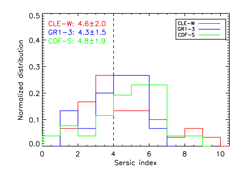
Figure 10.— Sérsic index distributions for our sample: red histogram is for cluster ETGs, blue histogram is for group ETGs and green histogram is for field ETGs. The dashed line represents a Sérsic index of 4, corresponding to a de Vaucouleurs profile. We also report the mean and standard deviation for the three distributions.

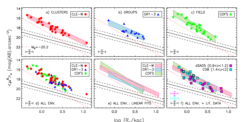
Figure 11.— Same as Figure 3, but with our sizes estimated with a de Vaucouleurs profile. Moreover, we include here in the local KR of Jorgensen et al. (1995) the three largest galaxies that we excluded in Figure 3. We observe that none of our conclusions of Section 4 is affected if we use de Vaucouleurs sizes.

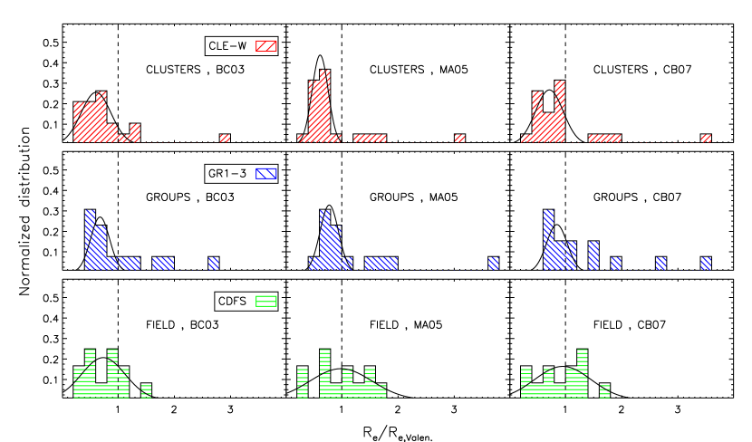
Figure 12.— Size ratio $R_{e}/R_{e,Valen}$ normalized distributions derived with the three stellar population models (BC03/MA05/CB07), split by environments: same figure as Figure 7, but we here remove ETGs known to have emission lines (7 ETGs in clusters, 4 ETGs in groups and 14 ETGs in the field). Our results do not change.

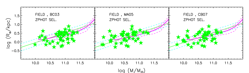
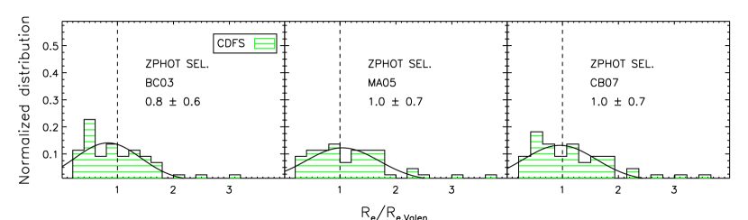
Figure 13.— Results when considering a CDF-S sample including ETGs with photometric redshift. Upper panels: MSR, symbols are as in Figure 6. Lower panels: size ratio $R_{e}/R_{e,Valen}$ normalized distributions derived with the three stellar population models (BC03/MA05/CB07), same as Figure 7. This sample shows a MSR similar to the local, as the spectroscopically selected sample. This test shows that our spectroscopically selected sample is not biased with respect to a photometric redshift selection.

References

- Bernardi et al. (2010) Bernardi, M., Shankar, F., Hyde, J. B., et al. 2010, MNRAS, 404, 2087
- Bernardi et al. (2003) Bernardi, M., Sheth, R. K., Annis, J., et al. 2003, AJ, 125, 1817
- Bertin & Arnouts (1996) Bertin, E. & Arnouts, S. 1996, A&AS, 117, 393
- Bezanson et al. (2009) Bezanson, R., van Dokkum, P. G., Tal, T., et al. 2009, ApJ, 697, 1290
- Blanton et al. (2005) Blanton, M. R., Eisenstein, D., Hogg, D. W., Schlegel, D. J., & Brinkmann, J. 2005, ApJ, 629, 143
- Bournaud et al. (2011) Bournaud, F., Chapon, D., Teyssier, R., et al. 2011, ApJ, 730, 4
- Bruzual & Charlot (2003) Bruzual, G. & Charlot, S. 2003, MNRAS, 344, 1000
- Buitrago et al. (2008) Buitrago, F., Trujillo, I., Conselice, C. J., et al. 2008, ApJ, 687, L61
- Caon et al. (1993) Caon, N., Capaccioli, M., & D’Onofrio, M. 1993, MNRAS, 265, 1013
- Cassata et al. (2011) Cassata, P., Giavalisco, M., Guo, Y., et al. 2011
- Cimatti et al. (2008) Cimatti, A., Cassata, P., Pozzetti, L., et al. 2008, A&A, 482, 21
- Conroy & Gunn (2010) Conroy, C. & Gunn, J. E. 2010, ApJ, 712, 833
- Daddi et al. (2005) Daddi, E., Renzini, A., Pirzkal, N., et al. 2005, ApJ, 626, 680
- Damjanov et al. (2009) Damjanov, I., McCarthy, P. J., Abraham, R. G., et al. 2009, ApJ, 695, 101
- de Vaucouleurs (1948) de Vaucouleurs, G. 1948, Annales d’Astrophysique, 11, 247
- di Serego Alighieri et al. (2005) di Serego Alighieri, S., Vernet, J., Cimatti, A., et al. 2005, A&A, 442, 125
- Djorgovski & Davis (1987) Djorgovski, S. & Davis, M. 1987, ApJ, 313, 59
- D’Onofrio et al. (2008) D’Onofrio, M., Fasano, G., Varela, J., et al. 2008, ApJ, 685, 875
- Dressler et al. (1987) Dressler, A., Lynden-Bell, D., Burstein, D., et al. 1987, ApJ, 313, 42
- Fan et al. (2008) Fan, L., Lapi, A., De Zotti, G., & Danese, L. 2008, ApJ, 689, L101
- Franx et al. (2008) Franx, M., van Dokkum, P. G., Schreiber, N. M. F., et al. 2008, ApJ, 688, 770
- Geller & Huchra (1983) Geller, M. J. & Huchra, J. P. 1983, ApJS, 52, 61
- Giavalisco et al. (2004) Giavalisco, M., Ferguson, H. C., Koekemoer, A. M., et al. 2004, ApJ, 600, L93
- Granato et al. (2006) Granato, G. L., Silva, L., Lapi, A., et al. 2006, MNRAS, 368, L72
- Häussler et al. (2007) Häussler, B., McIntosh, D. H., Barden, M., et al. 2007, ApJS, 172, 615
- Holden et al. (2005) Holden, B. P., Blakeslee, J. P., Postman, M., et al. 2005, ApJ, 626, 809
- Hopkins et al. (2009a) Hopkins, P. F., Bundy, K., Murray, N., et al. 2009a, MNRAS, 398, 898
- Hopkins et al. (2009b) Hopkins, P. F., Hernquist, L., Cox, T. J., Keres, D., & Wuyts, S. 2009b, ApJ, 691, 1424
- Hopkins et al. (2010) Hopkins, P. F., Bundy, K., Hernquist, L., Wuyts, S., & Cox, T. J. 2010, MNRAS, 401, 1099
- Jorgensen et al. (1995) Jorgensen, I., Franx, M., & Kjaergaard, P. 1995, MNRAS, 273, 1097
- Kaviraj et al. (2009) Kaviraj, S., Devriendt, J. E. G., Ferreras, I., Yi, S. K., & Silk, J. 2009, A&A, 503, 445
- Khochfar & Silk (2006) Khochfar, S. & Silk, J. 2006, MNRAS, 370, 902
- Kormendy (1977) Kormendy, J. 1977, ApJ, 218, 333
- Kron (1980) Kron, R. G. 1980, ApJS, 43, 305
- Kroupa (2001) Kroupa, P. 2001, MNRAS, 322, 231
- La Barbera et al. (2003) La Barbera, F., Busarello, G., Merluzzi, P., Massarotti, M., & Capaccioli, M. 2003, ApJ, 595, 127
- Longhetti et al. (2007) Longhetti, M., Saracco, P., Severgnini, P., et al. 2007, MNRAS, 374, 614
- Maltby et al. (2010) Maltby, D. T., Aragón-Salamanca, A., Gray, M. E., et al. 2010, MNRAS, 402, 282
- Mancini et al. (2010) Mancini, C., Daddi, E., Renzini, A., et al. 2010, MNRAS, 401, 933
- Maraston (2005) Maraston, C. 2005, MNRAS, 362, 799
- Maraston et al. (2006) Maraston, C., Daddi, E., Renzini, A., et al. 2006, ApJ, 652, 85
- McGrath et al. (2008) McGrath, E. J., Stockton, A., Canalizo, G., Iye, M., & Maihara, T. 2008, ApJ, 682, 303
- Mei et al. (2011) Mei, S., et al. 2011, ApJ, submitted
- Mei et al. (2009) Mei, S., Holden, B. P., Blakeslee, J. P., et al. 2009, ApJ, 690, 42
- Mei et al. (2006a) Mei, S., Blakeslee, J. P., Stanford, S. A., et al. 2006a, ApJ, 639, 81
- Mei et al. (2006b) Mei, S., Holden, B. P., Blakeslee, J. P., et al. 2006b, ApJ, 644, 759
- Naab et al. (2009) Naab, T., Johansson, P. H., & Ostriker, J. P. 2009, ApJ, 699, L178
- Nakata et al. (2005) Nakata, F., Kodama, T., Shimasaku, K., et al. 2005, MNRAS, 357, 1357
- Newman et al. (2010) Newman, A. B., Ellis, R. S., Treu, T., & Bundy, K. 2010, ApJ, 717, L103
- Nonino et al. (2009) Nonino, M., Dickinson, M., Rosati, P., et al. 2009, ApJS, 183, 244
- Onodera et al. (2010) Onodera, M., Daddi, E., Gobat, R., et al. 2010, ApJ, 715, L6
- Peng et al. (2002) Peng, C. Y., Ho, L. C., Impey, C. D., & Rix, H. 2002, AJ, 124, 266
- Poggianti et al. (2006) Poggianti, B. M., von der Linden, A., De Lucia, G., et al. 2006, ApJ, 642, 188
- Postman et al. (2005) Postman, M., Franx, M., Cross, N. J. G., et al. 2005, ApJ, 623, 721
- Raichoor et al. (2011) Raichoor, A., Mei, S., Nakata, F., et al. 2011, ApJ, 732, 12
- Rettura et al. (2010) Rettura, A., Rosati, P., Nonino, M., et al. 2010, ApJ, 709, 512
- Rettura et al. (2011) Rettura, A., Mei, S., Stanford, S. A., et al. 2011, ApJ, 732, 94
- Retzlaff et al. (2010) Retzlaff, J., Rosati, P., Dickinson, M., et al. 2010, A&A, 511, A50
- Rosati et al. (1999) Rosati, P., Stanford, S. A., Eisenhardt, P. R., et al. 1999, AJ, 118, 76
- Saglia et al. (2010) Saglia, R. P., Sánchez-Blázquez, P., Bender, R., et al. 2010, A&A, 524, A6
- Salimbeni et al. (2009) Salimbeni, S., Castellano, M., Pentericci, L., et al. 2009, A&A, 501, 865
- Salpeter (1955) Salpeter, E. E. 1955, ApJ, 121, 161
- Santini et al. (2009) Santini, P., Fontana, A., Grazian, A., et al. 2009, A&A, 504, 751
- Saracco et al. (2009) Saracco, P., Longhetti, M., & Andreon, S. 2009, MNRAS, 392, 718
- Saracco et al. (2010) Saracco, P., Longhetti, M., & Gargiulo, A. 2010, MNRAS, 408, L21
- Saracco et al. (2011) Saracco, P., Longhetti, M., & Gargiulo, A. 2011, MNRAS, 187
- Sérsic (1968) Sérsic, J. L. 1968, Atlas de galaxias australes (Observatorio Astronomico, Cordoba, Argentina)
- Shankar et al. (2011) Shankar, F., Marulli, F., Bernardi, M., et al. 2011, arXiv:1105.6043
- Shankar et al. (2010) Shankar, F., Marulli, F., Bernardi, M., et al. 2010, MNRAS, 405, 948
- Shankar et al. (2010) Shankar, F., Marulli, F., Bernardi, M., et al. 2010, MNRAS, 403, 117
- Shen et al. (2003) Shen, S., Mo, H. J., White, S. D. M., et al. 2003, MNRAS, 343, 978
- Simard et al. (2002) Simard, L., Willmer, C. N. A., Vogt, N. P., et al. 2002, ApJS, 142, 1
- Stanford et al. (1997) Stanford, S. A., Elston, R., Eisenhardt, P. R., et al. 1997, AJ, 114, 2232
- Strazzullo et al. (2010) Strazzullo, V., Rosati, P., Pannella, M., et al. 2010, A&A, 524, A17
- Taylor et al. (2010) Taylor, E. N., Franx, M., Glazebrook, K., et al. 2010, ApJ, 720, 723
- Toft et al. (2007) Toft, S., van Dokkum, P., Franx, M., et al. 2007, ApJ, 671, 285
- Trujillo et al. (2006) Trujillo, I., Feulner, G., Goranova, Y., et al. 2006, MNRAS, 373, L36
- Trujillo et al. (2007) Trujillo, I., Conselice, C. J., Bundy, K., et al. 2007, MNRAS, 382, 109
- Trujillo et al. (2009) Trujillo, I., Cenarro, A. J., de Lorenzo-Cáceres, A., et al. 2009, ApJ, 692, L118