MOKA: a new tool for Strong Lensing Studies

Abstract

Strong gravitational lensing is a powerful tool for probing the matter distribution in the cores of massive dark matter haloes. Recent and ongoing analyses of galaxy cluster surveys (MACS, CFHTLS, SDSS, SGAS, CLASH, LoCuSS) have adressed the question of the nature of the dark matter distribution in clusters. N-body simulations of cold dark-matter haloes consistently find that haloes should be characterized by a concentration-mass relation that decreases monotonically with halo mass, and populated by a large amount of substructures, representing the cores of accreted progenitor halos. It is important for our understanding of dark matter to test these predictions. We present MOKA, a new algorithm for simulating the gravitational lensing signal from cluster-sized haloes. It implements the most recent results from numerical simulations to create realistic cluster-scale lenses with properties independent of numerical resolution. We perform systematic studies of the strong lensing cross section as a function of halo structures. We find that the strong lensing cross sections depend most strongly on the concentration and on the inner slope of the density profile of a halo, followed in order of importance by halo triaxiality and the presence of a bright central galaxy.

1 Introduction

Galaxy clusters are an important probe for dark-matter properties. According to the standard scenario of structure formation, galaxy clusters as a population are still in their formation process. Since gas cooling cannot substantially compress dark matter haloes, their density profiles are dominated by dark matter.

Recent analyses of strong and weak lensing by galaxy clusters have found good consistence with an NFW-like profile whose projected mass density distribution continuously flattens towards the centre, as expected from CDM dominated haloes. However, for an increasing number of clusters Oguri et al. (2005); Oguri et al. (2009); Umetsu et al. (2011) have found that the mass-concentration relation seems to lie substantially above the relation predicted by CDM simulations. Strong lensing by clusters is sensitive to their internal structure – mass distribution within the Einstein radius, which includes (i) presence of substructure, (ii) asymmetry in their gravitational potential well, (iii) ellipticity, (iv) presence of a massive and bright central galaxy (v) inner slope of the dark matter density profile.

Apart from weak and strong lensing, the halo density profile can also be constrained from the velocity dispersion profile of the central galaxy (Sand et al., 2004; Newman et al., 2009) and X-ray emission from the hot intra-cluster gas. While gravitational lensing does not rely on any equilibrium or dynamical assumptions, methods based on galaxy or gas dynamics do, potentially biasing mass and concentration estimates.

In this paper, we shall quantify the importance of the structural parameters of dark matter haloes for strong lensing signal, using our new and fast algorithm MOKA (Matter density distributiOn Kode for gravitationAl lenses) to create realistic maps of substructured triaxial dark matter haloes, which are in perfect agreement with the measurements done on galaxy clusters extracted from numerical simulations.

In Section 2 we present the halo properties on which our algorithm relies. The halo lensing properties are presented in Section 2.2 and the strong lensing signal dependence on the halo modelling is discussed in Sections 3. Discussion and conclusion are presented in Section 4.

We adopt a $\mathrm{\Lambda CDM}$ model with $\Omega_{m}=0.3$, $\Omega_{\Lambda}=0.7$, $h=0.7$ and $\sigma_{8}=0.9$, consistently with the Mare Nostrum Universe that we compare some of our results to.

2 Construction of Realistic Lenses

Strong gravitational lensing depends on the matter distribution near halo centres where limited numerical resolution may affect the particle distribution. Here, we present a new algorithm, MOKA, which analytically creates surface mass density distributions of triaxial and substructured haloes independent of numerical resolution. MOKA is publicly available at the following url http://cgiocoli.wordpress.com/research-interests/moka. The idea behind this new algorithm is to construct realistic lenses starting from a set of ingredients taken from state of the art numerical simulations. It not only accounts for the smooth dark halo and stellar components, as earlier studies do (van de Ven et al., 2009; Mandelbaum et al., 2009), but also the presence of substructures perturbing the regular matter distribution. The procedure is discussed in the following subsections.

2.1 Host Halo Contents

Halo properties are described by the extended halo model Giocoli et al. (2010), developed for the reconstruction of the non-linear dark matter power spectrum. We briefly list its ingredients here.

2.1.1 Properties of the dark matter component

The virial mass of a halo is defined as

$$M_{vir}=\frac{4\pi}{3}R_{vir}^{3}\frac{\Delta_{vir}}{\Omega_{m}(z)}\Omega_{0}\rho_{c}\,,$$ (1)

where $\rho_{c}$ represents the critical density of the Universe, $\Omega_{0}=\Omega_{m}(0)$ the matter density parameter at the present time and $\Delta_{vir}$ is the virial overdensity (Eke et al., 1996; Bryan & Norman, 1998), $R_{vir}$ symbolizes the virial radius of the halo which defines the dinstance from the halo centre that encloses the desired density contrast. In what follows, we summarize the most recent numerical results built into MOKA.

• As said above, the dark matter density distribution in isolated haloes is well described by the NFW (Navarro et al., 1996) profile

  $$\rho(r|M_{vir})=\frac{\rho_{s}}{r/r_{s}(1+r/r_{s})^{2}}\,,$$ (2)

  where $r_{s}$ is the scale radius, defining the concentration $c_{vir}\equiv R_{vir}/r_{s}$, and $\rho_{s}$ is the dark matter density at the scale radius,

  $$\rho_{s}=\frac{M_{vir}}{4\pi r_{s}^{3}}\left[\ln(1+c_{vir})-\frac{c_{vir}}{1+c_{vir}}\right]^{-1}\,.$$ (3)

  Combining the preceding three equations, we can explicitly write the NFW profile as a function of $c_{vir}$ and $M_{vir}$,

  $$\rho(r|M_{vir}) = \dfrac{c_{vir}^{2}R_{vir}^{3}}{3r(R_{vir}+c_{vir}r)^{2}}\dfrac{\Delta_{vir}}{\Omega_{m}(z)}\Omega_{0}\rho_{c}$$ (4)

  $$\times \left[\ln(1+c_{vir})-\frac{c_{vir}}{1+c_{vir}}\right]^{-1}\,.$$

  We use this density profile to model the dark matter distribution in the clusters produced by MOKA.

• The halo concentration is a decreasing function of the host halo mass. This numerical result is explained in terms of hierarchical clustering in CDM and the different halo-formation histories. Already Bond et al. (1991) and Lacey & Cole (1993), following the extended-Press & Schechter (1974) theory, have found that the collapse time of dark matter haloes depends on the halo mass and that their assembly history is hierarchical: small systems collapse at higher redshifts than larger ones (Sheth & Tormen, 2004a; Giocoli et al., 2007). This trend is reflected in the mass-concentration relation: at a given redshift smaller haloes are more concentrated than larger ones. Different fitting functions for numerical mass-concentration relations have been given (Bullock et al., 2001; Neto et al., 2007; Duffy et al., 2008; Gao et al., 2008). In this work, we use the relation proposed by Zhao et al. (2009) which links the concentration of a given halo with the time ($t_{0.04}$) at which its main progenitor assembles $4$ percent of its mass,

  $$c_{vir}(M_{vir},z_{l})=4\left\{1+\left[\frac{t(z_{l})}{3.75t_{0.04}}\right]^{8.4}\right\}^{1/8}\,.$$ (5)

  The model by Zhao et al. (2009) fits well numerical simulations even with different cosmologies. It seems to be of reasonably general validity.

  Due to different assembly histories, haloes with same mass at the same redshift may have different concentrations (Navarro et al., 1996; Jing, 2000; Wechsler et al., 2002; Zhao et al., 2003a, b). At fixed host halo mass, the distribution in concentration is well fitted by a log normal distribution function with a variance $\sigma_{\ln c}$ between $0.1$ and $0.25$ (Jing, 2000; Dolag et al., 2004; Sheth & Tormen, 2004b; Neto et al., 2007).

• Halos are generally not spherical but triaxial due to their tidal interaction with the surrounding density field during their collapse (Sheth & Tormen, 1999, 2002). The correlation of the halo shape with the surrounding environment is expressed as a function of the matter density parameter and of the typical collapse mass. Jing & Suto (2002) have performed a statistical study of halo shapes extracted from numerical simulations, deriving that, if $a$, $b$ and $c$ represent the minor, median and major axes, respectively, empirical relations for $a/c$ and $a/b$ are given by the distribution

  $$p(\lambda)\mathrm{d}\lambda=\frac{1}{\sqrt{2\pi}\sigma_{\lambda}}\exp\left[-\frac{(\lambda-0.54)^{2}}{2\sigma_{\lambda}}\right]\mathrm{d}\lambda$$ (6)

  for $\lambda=(a/c)(M_{vir}/M_{*}(z_{l}))^{0.07\Omega(z_{l})}$ with $\sigma_{\lambda}=0.113$ and the conditional probability for the axis ratios

  $$p\left(a/b|a/c\right)=\left\{\begin{array}[]{ll}\frac{3}{2(1-r_{min}})\left[1-\left(\frac{2a/b-1-r_{min}}{1-r_{min}}\right)^{2}\right]&a/b\geq r_{min},\\ 0&a/b<r_{min},\\ \end{array}\right.$$

  where $r_{min}=0.5$ if $a/c<0.5$ else $r_{min}=a/c$. As usual, $M_{*}(z_{l})$ is the non-linear mass at redshift $z_{l}$. Simulations with gas cooling have produced haloes that tend to be more spherical than those in pure DM simulation (Kazantzidis et al., 2004). The host halo shape then depends also on the morphology of the stellar mass component. In this paper we use the prescriptions by Jing & Suto (2002), which are based on dark matter only simulations. However, MOKA is a very flexible tool, and the input distributions of axis ratios can be easily modified.

• Haloes are not smooth, but characterized by a large number of substructures, which may or not host satellite galaxies (Moore et al., 1999; Springel et al., 2001b; De Lucia et al., 2004). These substructures are cores of progenitor haloes accreted along the merger tree that were not completely disrupted by tidal stripping (Springel et al., 2001b; Gao et al., 2004; De Lucia et al., 2004; van den Bosch et al., 2005; Giocoli et al., 2008; Shaw et al., 2007). Because of different assembly histories and time scales for subhalo mass loss, more massive haloes retain more substructures than less massive haloes at a given redshift. Likewise, haloes with a lower concentration (and thus with a lower formation redshift) are on average more substructured than haloes with larger concentration. Giocoli et al. (2010a) fitted the subhalo mass function by

  $$\frac{1}{M_{vir}}\frac{\mathrm{d}N(M_{vir},c_{vir},z_{l})}{\mathrm{d}m}=$$

  $$A(1+z_{l})^{1/2}\frac{\bar{c}}{c_{vir}}m^{\alpha}\exp\left[-\beta\left(\frac{m}{M_{vir}}\right)^{3}\right]\,,$$ (7)

  where $A=9.33\times 10^{-4}$, $\beta=12.2715$, $\alpha=-0.9$ and $\bar{c}$ is the mean concentration of a halo with mass $M_{vir}$ at redshift $z_{l}$. We adopt this model because it incorporates the dependences of the subhalo mass function on the mass $M_{vir}$, the concentration $c_{vir}$ and the redshift $z_{l}$ of the host halo. To populate our haloes with substructures with mass $m_{i}$ we will randomly sample the distribution down to a minimal subhalo mass $m_{min}$.

  Subhalo density profiles are modified by tidal stripping due to close interactions with the main halo smooth component and to close encounters with other clumps, gravitational heating, and dynamical friction. Such events can cause the subhaloes to lose mass, and may eventually result in their complete disruption (Hayashi et al., 2003; Choi et al., 2007). The remaining self-bound subhaloes will have density profiles different from the NFW shape in that they are truncated at the tidal radius (Bullock et al., 2001). In order to take the truncation into account, we model the dark matter density distribution in subhaloes using truncated singular isothermal spheres (Keeton, 2003),

  $$\rho_{sub}(r)=\left\{\begin{array}[]{ll}\dfrac{\sigma_{v}^{2}}{2\pi Gr^{2}}&r\leq R_{sub},\\ 0&r>R_{sub}\\ \end{array}\right.$$

  with velocity dispersion $\sigma_{v}$, and $R_{sub}$ defined as:

  $$m_{sub} = \int_{0}^{R_{sub}}4\pi r^{2}\rho_{sub}(r)\mathrm{d}r\Rightarrow$$

  $$R_{sub} = \dfrac{G\,m_{sub}}{2\,\sigma_{v}^{2}}\,.$$ (8)

  The velocity dispersion $\sigma_{v}$ is related to the subhalo temperature by

  $$\sigma_{v}=f(T)\sigma_{v}^{(R)}+[1-f(T)]\sigma_{v}^{(T)}(T)\,,$$ (9)

  where

  $$f(T)=\left[1+\left(\dfrac{kT}{\mathrm{keV}}\right)^{4}\right]^{-1}\,.$$ (10)

  Based on the temperature definition in the spherical collapse model, we can write

  $$kT=(kT)_{15}M_{15}^{2/3}(1+z)\left(\dfrac{\Delta_{vir}\Omega_{0}}{18\pi^{2}\Omega_{m}(z)}\right)^{1/3}\,$$ (11)

  where $k$ is Boltzmann’s constant, and $M_{15}$ is the mass in units of $10^{15}\,M_{\odot}/h$. For temperatures much above $1$ keV, Eq. (9) follows the observed relation between X-ray temperature and velocity dispersion by Wu et al. (1998),

  $$\sigma_{v}^{(T)}=371.5\left(\dfrac{kT}{\mathrm{keV}}\right)^{0.56}\,\mathrm{km\,s^{-1}}\,;$$ (12)

  while for $T\ll 1$ keV it reduces to the relation

  $$\sigma_{v}^{(R)}=\left(\dfrac{Gm_{sub}H(z)\Delta_{vir}^{1/2}}{4}\right)^{1/3}$$ (13)

  that can be obtained combining Eqs. (8) and (1) identifying $R_{sub}=R_{vir}$.

  Let us define $R_{t}$ as the radius at which the subhalo mean density is of the order of the mean density of the main halo within $r$. Following Tormen et al. (1998) we can write it as:

  $$R_{t}=r\left[\dfrac{m_{sub}}{(2-\partial\ln M_{vir}(r)/\partial\ln r)M_{vir}(r)}\right]^{1/3}\,,$$ (14)

  where $m_{sub}$ and $r$ represent the subhalo mass and its distance from the host halo centre, and $M_{vir}(r)$ the host halo mass profile. Truncating subhaloes at $R_{sub}$ does not create discontinuities in the convergence map because $R_{t}(r)\lesssim R_{sub}$. It preserves the total subhalo mass fraction in hosts as found in numerical simulations (Gao et al., 2004; De Lucia et al., 2004; Giocoli et al., 2010a). If the host halo matter density distribution is described by an NFW-profile, the subhalo tidal radius as a function of the distance from the host halo centre can be analytically estimated. In Figure 1 we show the ratio between the subhalo tidal radius and the radius which encloses the subhalo mass as a function of the distance from the host halo centre. From the figure we notice that for $r<0.75R_{vir}$ $R_{t}\ll R_{sub}$ while when the subhalo is located near at the virial radius the ratio tends to unity.

  

  Figure 1: Ratio between the subhalo tidal radius and the one which encloses its mass as a function of the distance from the host halo centre. In the figure we show the case of three subhaloes located in a host halo with mass $10^{15}\,M_{\odot}/h$ at redshift $z=0.25$ with concentration $c_{vir}=4$.

  The SIS profile profile well represents galaxy density profiles on scales relevant for strong lensing. Previously, different authors have used this model to characterize the lensing signal by substructures after stripping (Metcalf & Madau, 2001). Nonetheless, additional subhalo density profiles will be implemented in MOKA to allow truncating the subhalo profile more smoothly.

• The spatial distribution of subhaloes tends to follow the smooth dark matter distribution of the host halo. However, clumps near the host halo center are easily destroyed, due to their tidal interaction with the main halo. Thus, the spatial subhalo distribution is less concentrated than the NFW profile of the host halo. Gao et al. (2004) have studied this using a cosmological numerical simulation and found that the cumulative spatial density distribution of clumps in host haloes is well described by

  $$\frac{n(<x)}{N_{tot}}=\frac{(1+\alpha^{\prime}c_{vir})x^{\beta^{\prime}}}{(1+\alpha^{\prime}c_{vir}x^{2})}\,$$ (15)

  where $x$ is the distance to the host halo centre in unit of the virial radius, $N_{tot}$ is the total number of subhaloes in the host, $\alpha^{\prime}=0.244$ and $\beta^{\prime}=2.75$. In the Figure 2 we show previouse equation for different value of the host halo concentration, as indicated in the label. To place sublumps in the host, we sample this distribution and randomly assign position angles $\theta$ and $\phi$ on a sphere. A similar equation has been used to model the satellite galaxy density distribution by van den Bosch et al. (2004).

  

  Figure 2: Radial subhalo density distribution model. The different curves show equation (15) for different values of the host halo concentration $c_{vir}$, as in the label.

2.1.2 Dissipative baryonic component and its effects on dark matter

Strong lensing is sensitive to the matter distribution inside the centre of galaxy clusters ($r\sim 100$ kpc). On such scales, the density of the baryonic component becomes comparable to that of the dark matter. Meneghetti et al. (2003) have shown that the brightest central galaxy (BCG) on strong lensing signal is generally moderately important for strong lensing, but potentially decisive for those haloes which are otherwise marginally supercritical strong lenses.

To populate haloes with a central galaxy of a certain stellar mass, we use the Halo Occupation Distribution (HOD) technique. HOD assumes that the stellar mass of a galaxy is tightly correlated with the depth of the potential well of the halo within which it formed, thus

$$M_{star}=\dfrac{2M_{star,0}}{(M_{infall}/M_{0})^{-\alpha"}+(M_{infall}/M_{0})^{-\beta"}}\,,$$ (16)

as estimated by Wang et al. (2006), who modelled this relation after the semi-analytic galaxy catalogue of the Millennium Simulation (Croton et al., 2006). In this relation, we include a Gaussian scatter in $M_{star}$ at a given host halo mass with $\sigma_{M_{star}}=0.148$. For the central galaxy, we set the parameters $\alpha"=0.39$, $\beta"=1.96$, and $\log(M_{star,0)}=10.35$.

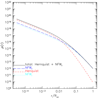
Figure 3: Density profile of a halo at $z_{l}=0.25$ with $M_{vir}=10^{15}M_{\odot}/h$. The dotted curve shows the NFW profile, the dashed curve the Henquist profile for the stellar component of the BCG at the halo centre with stellar mass $M_{star}=5\times 10^{12}M_{\odot}/h$. The dissipative baryon component modifies the dark-matter profile by adiabatic contraction as shown by the long-dashed line. The solid line shows the final profile.

For the stellar component of the BCG residing in the halo centre, we adopt the Hernquist (1990) profile

$$\rho_{star}(r)=\frac{\rho_{g}}{(r/r_{g})(1+r/r_{g})^{3}}\,.$$ (17)

It has a scale radius $r_{g}$ related to the half-mass (or effective) radius $R_{e}$ by $r_{g}=0.551R_{e}$, as done by Keeton (2001) we define the effective radius to be $R_{e}=0.03R_{vir}$. The scale density $\rho_{g}$ can be estimated by the definition of the total mass of a Hernquist model,

$$\rho_{s}=\frac{M_{star}}{2\pi r_{g}^{3}}\,.$$ (18)

The presence of a dissipative baryonic component influences the dark matter distribution near the host halo centre. Blumenthal et al. (1986) described the adiabatic contraction analytically, finding good agreement with numerical simulations. The initial and final density profiles – characterized by an initial radius $r_{i}$ and a final radius $r_{f}$, when a central galaxy is present – are related by

$$r\left[M_{star}(r)+M_{DM,f}\right]=r_{i}M_{DM,i}(r_{i})\,,$$ (19)

where

$$M_{DM,f}=M_{DM,i}\left(1-f_{cool}\right)\,,$$ (20)

and $f_{cool}$ is the baryon fraction in the halo that cools to form the central galaxy. To solve the adiabatic-contraction equation, we need to derive $r$ from equation (19). With a Hernquist model,

$$f_{cool}r^{3}+(r+r_{g})^{2}\left[(1-f_{cool})r-r_{i}\right]m_{i}(r_{i})=0\,;$$ (21)

This equation has a single relevant real root. We recall that $m_{i}$ in the previous equation defines the initial mass profile normalized by the virial mass. Figure 3 shows the density profile of a halo with virial mass $M_{vir}=10^{15}M_{\odot}/h$ and $c_{vir}=4$ populated with a galaxy with stellar mass $M_{star}=5\times 10^{12}M_{\odot}/h$. The dotted and short-dashed curves refer to the initial dark matter and stellar density in the halo, respectively. The presence of a dissipative baryonic component contracts the dark matter distribution. Solving Eq. (21), the dark matter density profile changes to the long-dashed curve. The solid curve shows the total density distribution obtained by summing the short and the long-dashed curves. We recall that for DM-only realizations, $M_{vir}$ is given by the sum in smooth plus clumpy components, while $M_{vir}=M_{smooth}+\sum_{i=1}^{N_{tot}}m_{i}+M_{star}$ if a BCG is present.

2.2 Halo Lensing Properties

In this section we will describe how we calculate lensing properties starting from the 3D matter density of all components characterising the haloes. For each component, we project the density on a plane perpendicular to the line of sight,

$$\Sigma(x,y)=\int_{-\infty}^{\infty}\rho(x,y,z)\mathrm{d}z\,,$$ (22)

where $r=\sqrt{x^{2}+y^{2}+z^{2}}$ with the coordinate origin put into the host halo centre, and defining $\xi=\sqrt{x^{2}+y^{2}}$.

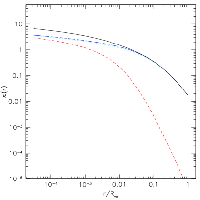
Figure 4: Convergence profile of the same cluster, assuming sources at redshift $z_{s}=2$.

The projected mass density of the NFW, Hernquist and SIS profiles can be given analytically (Bartelmann, 1996; Bartelmann & Schneider, 2001; Keeton, 2001):

$$\Sigma_{NFW}(x,y)=\frac{2\rho_{s}r_{s}}{\zeta^{2}-1}F(\zeta)\,,$$ (23)

$$\Sigma_{star}(x,y)=\rho_{g}r_{g}\frac{(2+\eta^{2})G(\eta)-3}{(\eta^{2}-1)^{2}}\,,$$ (24)

$$\Sigma_{sub}(x,y)=\frac{\sigma_{v}}{2G\xi}\,,$$ (25)

where $\zeta\equiv\xi/r_{s}$, $\eta\equiv\xi/r_{g}$, and the two functions $F(\zeta)$ and $G(\eta)$ are

$$F(\zeta)=\left\{\begin{array}[]{ll}1-\frac{2}{\sqrt{\zeta^{2}-1}}\arctan\sqrt{\dfrac{\zeta-1}{\zeta+1}}&\zeta>1,\\ 1-\frac{2}{\sqrt{1-\zeta^{2}}}\mathrm{arctanh}\sqrt{-\dfrac{\zeta-1}{\zeta+1}}&\zeta<1,\\ 0&\zeta=1;\\ \end{array}\right.$$

$$G(\eta)=\left\{\begin{array}[]{ll}\frac{1}{\sqrt{\eta^{2}-1}}\tan^{-1}\sqrt{\eta^{2}-1}&\eta>1,\\ \frac{1}{\sqrt{1-\eta^{2}}}\tanh^{-1}\sqrt{1-\eta^{2}}&\eta<1,\\ 1&\eta=1.\\ \end{array}\right.$$

We recall that the subhalo density profile is truncated at the radius enclosing its total (bound) mass. The convergence is the appropriately scaled surface mass density $\Sigma(x,y)$,

$$\kappa(x,y)=\frac{\Sigma(x,y)}{\Sigma_{cr}}\,$$ (26)

where

$$\Sigma_{cr}=\frac{c^{2}}{4\pi G}\frac{D_{s}}{D_{l}D_{ls}}\,,$$ (27)

is the critical surface mass density, containing the angular-diametre distance $D_{l}$, $D_{s}$ and $D_{ls}$ from the observer to the lens, to the source, and from the lens to the source, respectively.

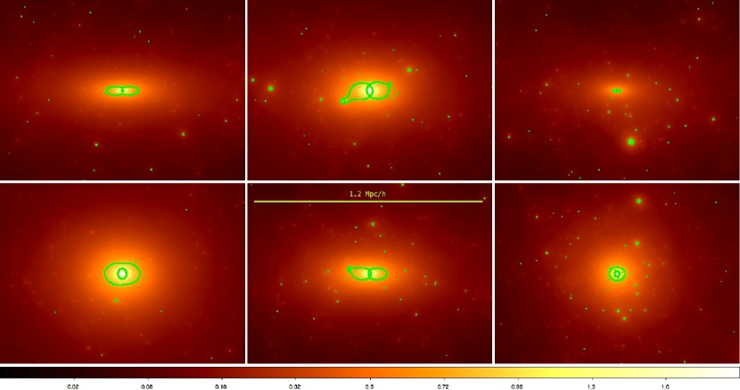
Figure 5: Convergence maps of cluster-sized haloes created with our MOKA code at redshift $z_{l}=0.25$, assuming sources at the single redshift $z_{s}=2$. The solid curves indicate the tangential and radial critical curves. All haloes have a virial mass of $10^{15}M_{\odot}/h$ and a minimum subhalo mass of $10^{10}\,M_{\odot}/h$.

Figure 4 shows the convergence profiles for the halo components presented in Figure 3, with sources assumed at $z_{s}=2$.

For each dark-matter halo, the total convergence map is the sum of all contribution maps,

$$\kappa(x,y)=\kappa_{DM}(x,y) +$$ (28)

$$\kappa_{star}(x,y) + \sum_{i=1}^{N}\kappa_{sub,i}(x-x_{c},y-y_{c})\,,$$

where $x_{c}$ and $y_{c}$ represent the center of mass of the $i$-th substructure. To introduce ellipticity into our model, we draw random numbers from the Jing & Suto (2002) distributions for the axial ratios $a/b$ and $a/c$, requiring $abc=1$. Once the axial ratios are known, we deform the convergence map accordingly. To randomly orient the halo, we choose a random point on a sphere identified by its azimuthal and elevation angles and rotate the halo ellipsoid by these angles. We assign the same projected ellipticity to the smooth component, to the stellar density and to the subhalo spatial density distributions. For the dark matter density distribution in subhaloes we assume spherically symmetric models, this because the subhalo typical scale is much smaller than the virial radius of the host system in which they are located. Having elliptical subhaloes will impact slightly on the total strong lensing cross-section. We have chosen to assign the same ellipticity to the BCG and to the dark matter density distribution in the host following the results of Fasano et al. (2010) who found that the shape of the BCG tends to reflect that of the associated dark matter halo. Figure 5 show the convergence maps of six galaxy clusters generated with our algorithm. All haloes are located at redshift $z=0.25$ and possess a virial mass equal to $10^{15}M_{\odot}/h$. The source redshift is $z_{s}=2$. The subhalo mass resolution is $10^{10}\,M_{\odot}/h$. This ensures a substructure mass fraction compatible with Richard et al. (2010), and consistent with the fact that systems with a lower substructure fraction tend to form at higher redshift, and are thus more concentrated (Smith & Taylor, 2008).

From the convergence map, the effective potential and the scaled deflection angle can be obtained by means of the equations

$$\Phi(x,y)=\frac{1}{\pi}\int_{\mathbb{R}^{2}}\kappa(\vec{\xi}^{\prime})\ln|\vec{\xi}-\vec{\xi}^{\prime}|\mathrm{d}^{2}\xi^{\prime},$$ (29)

and

$$\alpha(x,y)=\frac{1}{\pi}\int_{\mathbb{R}^{2}}\kappa(\vec{\xi}^{\prime})\frac{\vec{\xi}-\vec{\xi}^{\prime}}{|\vec{\xi}-\vec{\xi}^{\prime}|}\mathrm{d}^{2}\xi^{\prime}.$$ (30)

A source will be seen at the angular position $\vec{\theta}$ related to its intrinsic angular position $\vec{\beta}$ by the lens equation

$$\vec{\beta}=\vec{\theta}-\vec{\alpha}(\vec{\theta}).$$ (31)

Derivatives of the lensing potential are denoted by subscripts,

$$\frac{\partial^{2}\Phi(x,y)}{\partial\xi_{i}\partial\xi_{j}}\equiv\Phi_{ij},$$ (32)

where $\xi_{i}=x$ when $i=1$ and $\xi_{i}=y$ when $i=2$. We introduce the pseudo-vector field of the shear $\vec{\gamma}=(\gamma_{1},\gamma_{2})$ by its components

$$\gamma_{1}(x,y) = \frac{1}{2}(\Phi_{11}-\Phi_{22}),$$ (33)

$$\gamma_{2}(x,y) = \Phi_{12}=\Phi_{21}.$$ (34)

Light bundles are deflected differentially and thus distorted as described by the Jacobian matrix

$$A=\left(\delta_{ij}-\Phi_{ij}\right),$$ (35)

with the eigenvalues

$$\lambda_{t} = 1-\kappa-\gamma,$$ (36)

$$\lambda_{r} = 1-\kappa+\gamma.$$ (37)

The conditions $\lambda_{t}=0$ and $\lambda_{r}=0$ define the location of the tangential and radial critical curves in the lens plane, where the magnification is formally infinite. Mapping the critical curve back into the source plane by the lens equation gives the tangential and radial caustics.

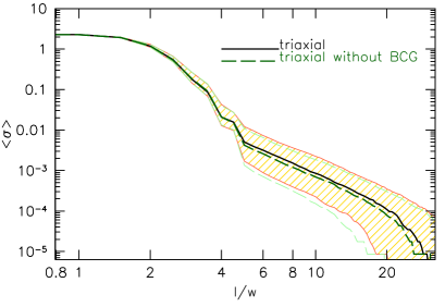
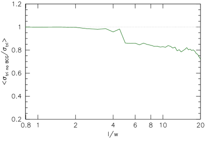
Figure 6: Left panel: median of the strong lensing cross sections $\sigma$ of a sample of simulated haloes with $10^{15}M_{\odot}/h$ at $z_{l}=0.25$ with sources at $z_{s}=2$ as a function of $l/w$. The solid curves show the median and $25-75\%$ percentiles of $\sigma$ for triaxial haloes with a BCG, while the dashed curves are the same sample but with only DM components. Right panel: median ratio of the strong lensing cross section without and with BCG as function of $l/w$. The scatter for $l/w>5$ is of the order of $0.4$.

Table 1 summarizes the list of parameters controlling MOKA.

Table 1: List of parameters present in MOKA 1.0: http://cgiocoli.wordpress.com/research-interests/moka.

Halo concentration:	drawn from a log-normal distribution around the mean value at fixed mass1
Halo virial radius:	defined from the spherical collapse model
Axial ratios:	drawn from the Jing & Suto (2002) model2
Halo orientation:	random picking the point on a sphere
Subhalo mass function:	random sampling the Giocoli et al. (2010a) model
Subhalo distribution:	random sampling the Gao et al. (2004) model, also NFW model has been implemented
Subhalo velocity dispersion:	fixed by the equation (9)
BCG stellar mass:	sampling the Wang et al. (2006) model with a gaussian scatter
BCG effective radius:	fixed to be the $4\%$ of the host halo virial radius (Keeton, 2001)

¹MOKA is flexible being able to work with different mass-concentration relation model

²ellipticity can be turned off

3 Lens structural properties and strong lensing signals

In this section we discuss the strong lensing efficiency of clusters produced by MOKA. Most of the discussion is focussed on the lensing cross section $\sigma$. This is defined as the region on the source plane from where the sources are mapped into images with a certain length-to-width ration $l/w$.

For each cluster we create a high-resolution deflection angle map of $2048\times 2048$ pixels centred on the cluster centre, with side length equal to the virial radius. From this we numerically estimate the lensing cross section by means of ray-tracing methods (Meneghetti et al., 2005a; Meneghetti et al., 2005b; Fedeli et al., 2006; Meneghetti et al., 2011). A typical calculation takes about one minute on a $3.06$ GHz single-core processor. Starting from the observer, bundles of light rays are traced back to the source plane. Using an adaptive grid, this is populated by elliptical sources of a fixed equivalent radius of $0.5^{\prime\prime}$. The number of highly magnified images is increased by refining the spatial resolution on the source plane near caustics. Analysing the images individually and measuring their length-width ratio $l/w$, we can define the lensing cross section for giant arcs $\sigma_{l/w}$ as the region on the source plane from where the sources are mapped into images with a certain $l/w$. Giant arcs are commonly defined as distorted images with a length-to-width ratio $l/w\geq 7.5$ or $l/w\geq 10$. We shall discuss our results for the three different values $l/w=5$, $7.5$ and $10$.

The integral of the strong lensing cross section of a galaxy cluster for different $z_{s}$, weighted by a source redshift distribution, allows to quantify the number of gravitational arcs expected to be seen. The strong lensing analysis of galaxy cluster size haloes from a $\mathrm{\Lambda}$CDM numerical simulations by Bartelmann et al. (1998) has revealed that those haloes produce an order of magnitude fewer gravitational arcs than observed. Studying how strong lensing cross sections change with structural halo properties may help to understand possible current limitations of numerical simulations, without the need of advocating cosmological models with dark energy (Bartelmann et al., 2003).

Recent observational studies of strong lensing clusters revealed that observed clusters seem to be more concentrated than simulated clusters. This causes more prominent strong lensing features. In the following, we shall quantify how much the presence of a BCG and halo triaxiality influence the strong lensing cross section for giant arcs. We have created a sample of $128$ high-resolution convergence maps of haloes with mass $10^{15}\,M_{\odot}/h$ and sources located at a fixed redshift $z_{s}=2$. This study is considered as a reference starting point to present our code MOKA. At the present time we are performing a statistical analysis of haloes in a $\mathrm{\Lambda}CDM$ universe to give an estimate of the strong lensing cross section as a function of redshift and of the halo abundance (Boldrin et al. in preparation).

3.1 BCG

Using a variety of Gas-dynamical simulations, Puchwein et al. (2005) studied the impact of the gas component on strong lensing signals, finding that the formation of stars mainly in the central region of the cluster tends to increase the cross section by about $20-30\%$, depending on lens redshift. To consider an analogous case, we have generated a sample of haloes with the same structural properties ($M_{vir}=10^{15}M_{\odot}/h$, $z_{l}=0.25$ and $z_{s}=2$), with and without a central galaxy. We recall that for pure dark matter lenses the virial mass takes into account the sum of the smooth plus clump components, while in simulations with BCG the total $M_{vir}$ includes also the presence of the stellar system. In both cases, the total masses are identical. For each halo we have post-processed their deflection angle map and estimated the strong lensing cross sections as a function of arc length-to-width ratio $l/w$. The left panel of Figure 6 shows the median strong lensing cross section as a function of $l/w$ for a sample of clusters with (solid) and without BCG (dashed curve). The shaded regions enclose $25-75\%$ of the data. The right panel of the same figure shows for each cluster the ratio of the strong lensing cross section as function of length-to-width ratio with and without a BCG, including the estimated median. The Figure confirms that at redshift $z_{l}=0.25$, the value of $\sigma$ for arcs with length-to-width ratio $l/w>5$ tends to be lower of a $20\%$ when the BCG is not included.

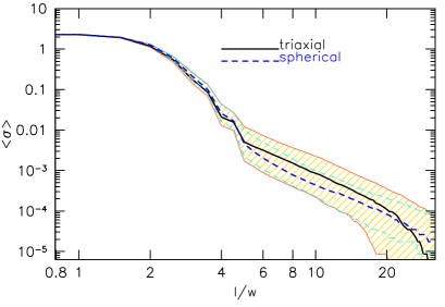
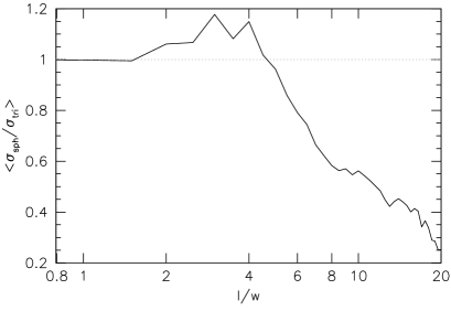
Figure 7: Left panel: median of the strong lensing cross sections $\sigma$ of a sample of simulated haloes with $10^{15}M_{\odot}/h$ at $z_{l}=0.25$ with sources at $z_{s}=2$ as function of $l/w$. The solid line shows the median and the $25-75\%$ percentiles of $\sigma$ for triaxial haloes (same as Fig. 6), while the dashed line is for spherical haloes. BCGs are present in both samples. Right panel: median of the ratio of the strong lensing cross section for the trixial and spherical haloes as function of $l/w$. Neglecting triaxiality decreases the singal for $l/w>5$ by $20-70\%$. The scatter for $l/w>5$ is of the order of $0.4$.

3.2 Triaxiality

Now we consider the case of spherical and triaxial haloes. Triaxiality affects strong lensing through the halo orientation. A cluster whose major axis is oriented along the line of sight will be a more efficient strong lens than if it is oriented otherwise. This orientation bias influences also mass and concentration estimates (Meneghetti et al., 2010b). To quantify how important triaxiality is for the appearance of giant arcs, we have created a sample of spherical haloes and compared their strong lensing cross sections to those of our fiducial sample of triaxial haloes whose mean ellipticity is $\epsilon_{3D}=0.15$. Figure 7 shows the strong lensing cross section as a function of $l/w$ for the same sample of either triaxial or spherical galaxy-cluster haloes. Both samples contain BCGs. The right panel shows the median ratio of $\sigma$ between the two samples: for $l/w>5$, the strong-lensing signal tends to decrease by between $20\,\%$ and $70\,\%$ in spherical compared to triaxial haloes. This confirms results obtained with a small sample of simulated haloes by Meneghetti et al. (2007b). Notice also that arcs with small length-to-width ratios (between $2$ to and $5$) are more abundant in spherical haloes because of their relatively lower shear.

3.3 Scatter

At a given host halo mass and lensing redshift, the strong lensing cross section scatters around its mean. This scatter is due to both halo triaxiality, presence and distribution of substructures and concentrations. Fedeli et al. (2010) fit the scatter in $y=\log(\sigma_{7.5})$ for galaxy cluster sized haloes with a Gaussian distribution, or an Edgeworth expansion around it, including skewness. Figure 8 shows the distribution of the strong lensing cross sections for three length-to-width ratios $l/w=5$, $7.5$ and $10$. In all cases, Gaussian distributions fit the data well with no significant deviation from the Edgeworth expansion, which we superpose. The distributions have standard deviation of $\sigma_{\log(\sigma)}$ slightly increasing with $l/w$; we find $\sigma_{\log(\sigma)}=0.56$, $0.59$ and $0.61$ for $l/w=5$, $7.5$ and $10$, respectively. These values are approximately twice those found by Fedeli et al. (2010). We believe that the main reason for the larger standard deviation is how the halo boundaries were defined in the simulations and with our algorithm: while we include all matter of the main halo along the line of sight, Fedeli et al. (2010) have extracted boxes of $5$ Mpc side length from their simulation. Another contribution to this difference is given by the fact that for each halo Fedeli et al. (2010) estimate the strong lensing cross section as mean of the three projections: at the end this procedure cuts the wings of their distribution.

3.4 Concentration

Haloes of the same mass have different concentrations reflecting their different assembly histories. We show in Appendix A how the rms scatter in the strong lensing cross sections is related to the concentration scatter and thus to the different host halo merger histories.

Strong lensing depends mainly on the matter density in the cluster cores, where the dark-matter density profile approaches a logarithmic slope near $-1$. The scale where the logarithmic density slope is $-2$ defines the scale radius $r_{s}$ and the host halo concentration by $c_{vir}=r_{s}/R_{vir}$. Higher concentrations cause larger strong lensing cross sections. Figure 9 shows this relation for our halo sample at $z_{l}=0.25$. Filled triangles show the median of the relation, with error bars enclosing the quartile of the distribution in each $\sigma_{7.5}$ bin. The solid line shows a least-squares fit to the data whose slope is $2.83\pm 0.06$. The dashed curve shows the predicted relation between the strong lensing cross section and the host halo concentration for spherical smooth NFW haloes with mass $10^{15}M_{\odot}/h$. Notice that our simulated lenses tend to have larger strong lensing cross sections at low concentration compared to spherical NFW haloes. This is mainly due to the BCGs and triaxiality which both tend to increase the projected central mass density.

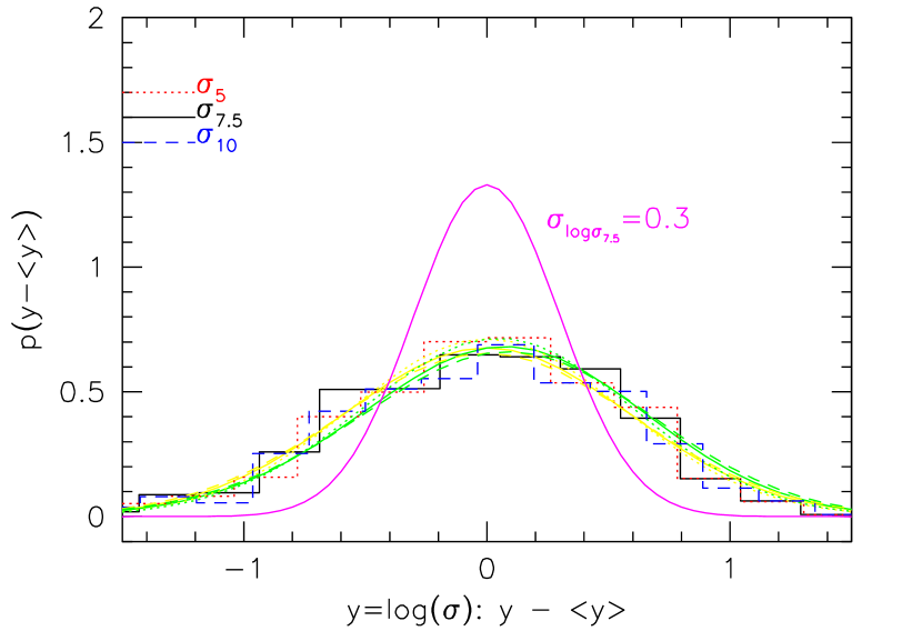
Figure 8: Distribution of the strong lensing cross section at $l/w=5$, $7.5$ and $10$. To fit the distributions, we have considered both a Gaussian and an Edgeworth expansion, for $y=\log(\sigma)$, which are superposed for corresponding value of $\sigma_{l/w}$. The solid line shows a Gaussian with $\sigma=0.3$.

Figure 9: Correlation between the strong lensing cross section for arcs with length-to-width ratio $\geq 7.5$ and the host halo concentration. Filled triangles show the median of the correlation and the shaded region encloses $25-75\%$ of the data. The solid line is a least-squares fit to these data points whose slope is $2.83\pm 0.06$. The dashed curve shows the prediction for spherical and smooth NFW haloes (without a central galaxy). In this case the sample of haloes is made up of $1024$ systems with mass $M_{vir}=10^{15}\,M_{\odot}/h$ at redshift $z_{l}=0.25$.

3.4.1 Statistical Properties

To summarize, we discuss now the strong lensing efficiency of a population of clusters generated with MOKA and we compare it to that of a similar sample of numerically simulated cluster taken from a cosmological box.

Meneghetti et al. (2010a) studied the strong lensing by a sample of galaxy clusters from the MARE NOSTRUM UNIVERSE. In Figure 10, we compare our findings with the median cross section of a sample of simulated haloes with masses between $6-7\times 10^{14}M_{\odot}/h$ at redshift $z_{l}=0.18$ (filled circle). Since the MARE NOSTRUM simulation does not include radiative processes and star formation, haloes formed therein do not contain a central massive galaxy. To make them compatible with the MOKA haloes, we add a BCG with mean $10^{12}\,M_{\odot}/h$ at their center. The solid line shows the median cross section (shaded regions enclose $25-90\%$ and $90-100\%$ of the data) for a sample of MOKA haloes in the same mass range, whose abundance has been weighted by the Sheth & Tormen (1999) mass function. The three solid curves show the same regions for the haloes in the MARE NOSTRUM UNIVERSE. Our algorithm well reproduces the median of the strong lensing cross sections measured in the numerical simulation. It doesn’t reproduce the scatter of the lensing cross sections for the reasons discussed above.

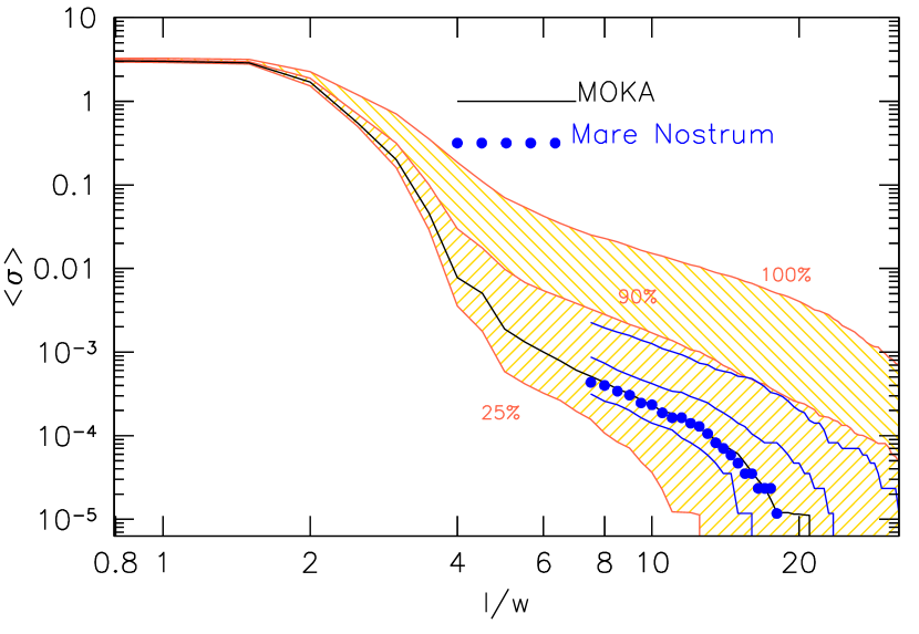
Figure 10: Comparison between the median strong lensing cross section $\sigma$ as a function of $l/w$ measured in analytically modelled haloes (solid line) and in haloes from the MARE NOSTRUM UNIVERSE (filled circles) for a sample of cluster-sized haloes in the mass range $6-7\times 10^{14}M_{\odot}/h$. The shaded regions enclose $25\%-90\%$ and $90\%-100\%$ for a sample of MOKA haloes, while the three solid curves illustrate the same regions for the haloes in the MARE NOSTRUM UNIVERSE.

3.4.2 Host halo concentration

Recent studies combining strong and weak lensing of galaxy clusters have not only disagreed with predictions of the number of arcs, but the observed clusters also seem to have Einstein radii larger than predicted in the $\mathrm{\Lambda CDM}$ cosmology (Zitrin et al., 2011a; Zitrin et al., 2011c). This may emphasise that observed clusters are more concentrated than those found in numerical simulations (Oguri et al., 2005; Oguri et al., 2009). However, over-concentrations in observed haloes may also result from an orientation bias (Meneghetti et al., 2011).

We shall now quantify by how much the strong lensing signal changes if the normalization of the mass-concentration relation is increased. We perform different simulations of the same halo sample, assuming that the mass-concentration relation is given by Eq. (5), where we include a normalization factor $c_{0}$. A reasonable choice for $c_{0}$ is a value between $-3.2$ and $6.4$, consistently with simulation results for the mean concentration scatter at fixed halo mass.

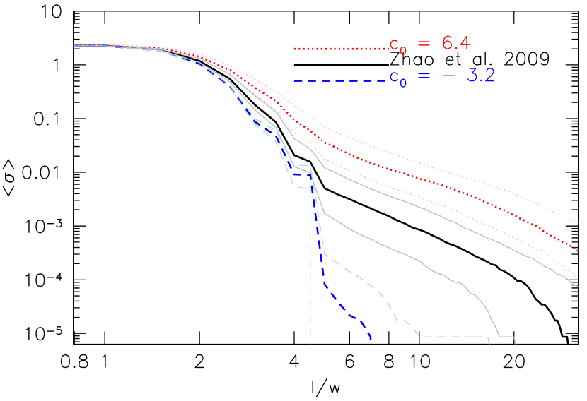
Figure 11: Dependence of the median strong lensing cross section on the normalization of the mass-concentration relation. The solid line shows the median cross section for our fiducial sample of cluster at $z_{l}=0.25$, the dotted and the dashed lines show the relation for higher and lower value of the normalization in the mass-concentration relation relation: $c_{vir}^{\prime}(M_{vir},z_{l})=c_{vir}(M_{vir},z_{l})+c_{0}$, for Zhao et al. (2009) $c_{0}=0$.

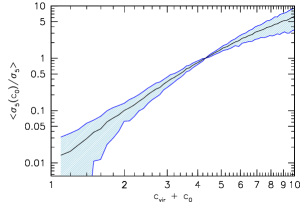
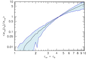
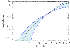
Figure 12: The median ratio of the strong lensing cross section with respect to the fiducial sample as a function of the normalization $c_{vir}+c_{0}$ in the Zhao et al. (2009) mass concentration relation for three different value of $l/w=5$, $7.5$ and $10$ in the left, central and right panels, respectively. The shaded region is enclosed by the lower and the upper quartiles.

Figure 12 shows the median ratio of strong lensing cross sections with our fiducial sample as a function of $c_{vir}^{\prime}=c_{vir}+c_{0}$ for $l/w=5$, $7.5$ and $10$. A higher normalization tends to increase strong lensing. Going from a mean value of the concentration for cluster size haloes from $4$ to $8$, the strong lensing cross section increases by about a factor of $4$.

3.5 Subhalo abundance

Torri et al. (2004) have shown that merger events and substructures increase the strong lensing cross sections, mostly if the latter are located near the cluster centre.

Our analysis has so far used cluster maps whose subhalo mass function was obtained by sampling the distribution 7 down to $10^{10}M_{\odot}/h$. To statistically analyse how the strong lensing signal depends on the minimum subhalo mass in our models, we have generated a sample of triaxial haloes with BCG, sampling the subhalo mass function down to a variable minimum mass $m_{min}$. The total halo mass $M_{vir}=10^{15}M_{\odot}/h$ is kept fixed.

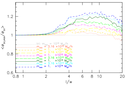
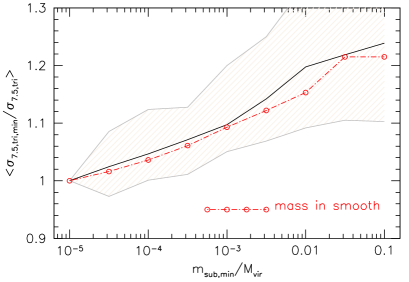
Figure 13: The dependence of the strong lensing cross section on the minimum subhalo mass. Left panel: median strong lensing cross section scaled by the fiducial triaxial simulation with subhalo mass resolution $10^{10}M_{\odot}/h$. Right panel: median rescaled cross section at $l/w=7.5$ as a function of the minimum subhalo mass. The median rescaled strong lensing cross sections for $l/w=5$ and $10$ as a function of $m_{min}/M_{vir}$ do not fall far away from the one estimated for $l/w=7.5$. The data points connected with a dot-dashed line show the median of the host halo smooth mass component rescaled with respect to the smooth mass component when the minimum subhalo mass is $10^{10}M_{\odot}/h$, as a function of the minimum subhalo mass.

Figure 13 shows the strong lensing signal as a function of the minimum subhalo mass. The left panel shows the median ratio of runs with different resolutions compared to the fiducial case, whose subhalo mass is $\geq 10^{10}M_{\odot}/h$. The strong lensing signal increases when the minimum subhalo mass changes from $10^{10}M_{\odot}/h$ to $10^{14}M_{\odot}/h$ because the smooth halo mass tends to increase for larger value of $m_{min}$, raising the projected mass density distribution near the host halo centre. The right panel shows the ratio $\langle\sigma_{min}/\sigma\rangle$ at $l/w=7.5$ as a function of the minimum subhalo mass expressed in terms of the total mass. Again, the strong lensing signal increases because the smooth component contains more mass. This is shown in the same figure, where the data points show the median of the smooth mass component in the host halo as a function of the minimum subhalo mass, rescaled with respect to the smooth mass component, with a minimum subhalo mass of $10^{10}M_{\odot}/h$.

Notice that the strong lensing cross section depends on the minimum subhalo mass. A decrease of the latter by a factor of $10$ tends to increase $\sigma_{7.5}$ by $5\%$ because the smooth mass increases. However, the impact of substructures can be different in different clusters depending of the particular configuration of the lens

3.6 Generalized NFW density profile

One of the main potential problems of the CDM model regards the inner slope of halo density profiles. Studying a sample of six strongly lensing clusters, Sand et al. (2004) concluded that, at $68\,\%$ confidence, the inner slope is consistent with $\beta\approx 0.52$ and that this is inconsistent with $\beta=1$ at the $99\,\%$ level. Recent analyses by Newman et al. (2009); Newman et al. (2011) of Abell 611 and 383 have confirmed a flat central dark matter density profile. How much does the inner slope bias the strong lensing signal?

To answer this question we have generated a sample of haloes with different $\beta$. We take adiabatic contraction in the center into account by means of Eq. (21), where $m_{i}(r_{i})$ is estimated by integrating equation (38).

The generalized NFW density profile

$$\rho_{gNFW}=\frac{\rho_{s}}{(r/r_{s})^{\beta}(1+r/r_{s})^{3-\beta}}\,,$$ (38)

is taken to have an arbitrary inner slope $\beta$. We define $r_{-2}\equiv(2-\beta)r_{s}$ and the concentration $c_{-2}=c_{vir}/(2-\beta)$ at the radius where the density profile is isothermal.

Figure 14 shows the median strong lensing cross section for three samples of cluster sized haloes. $NFW$ labels our fiducial sample with $\beta=1$, while $\beta=1.5$ and $0.5$ illustrate a steeper and a shallower profile.

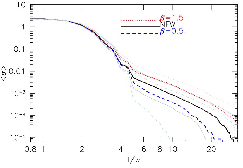
Figure 14: The median value of the strong lensing cross section for three different values of the inner slope of the density profile of the host. Dotted, solid and dashed line refer to a sample of haloes with $\beta=1.5$, $1$ and $0.5$, respectively. The thin solid curves show the quartiles of the NFW sample.

The three panels in Fig. 15 show the relation between the median ratio of the strong lensing cross section at $l/w=5$, $7.5$ and $10$ compared to our fiducial sample as function of the inner slope $\beta$. In each panel the shaded region encloses the lower and the upper quartiles, while the dashed line shows the least-squares fit to the data,

$$\log\left(\langle\sigma(\beta)/\sigma_{NFW}\rangle\right)=a\cdot\beta+b\,,$$ (39)

for which we find

$$a=0.572\pm 0.005,\;b=-0.560\pm 0.005\quad \sigma_{5}$$

$$a=0.710\pm 0.005,\;b=-0.701\pm 0.006\quad \sigma_{7.5}$$

$$a=0.768\pm 0.009,\;b=-0.750\pm 0.009\quad \sigma_{10}$$ .

A shallower (steeper) inner slope tends to decrease (increase) the strong lensing cross section with $l/w>5$ by about $50\%$ ($100\%$). Consindering triaxial haloes with $\beta=1$ and $\beta=1.5$, analogous values for the strong lensing cross section for $l/w=7$ and $l/w=10$ and sources with $z_{s}<1.25$ have been found by Oguri et al. (2003).

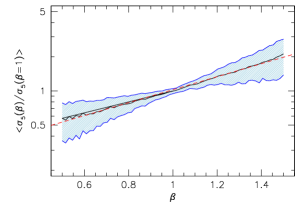
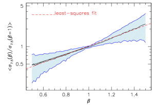
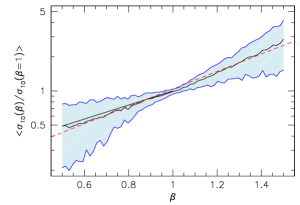
Figure 15: The median ratio of the strong lensing cross section as function the inner slope of the main halo density profile for $l/w=5$, $7.5$ and $10$. In each panel the shaded region enclose $25-50\%$ of the data and the dashed line the least-squares fit to the correlation.

4 Conclusions

We have presented a new algorithm to study the lensing signal from cluster sized haloes. The ingredients that we use to build up our triaxial and substructured models take into account the most recent results from numerical simulations of structure formation. The possibility of turning these ingredients on and off in our algorithm allows us to quantify the importance of all halo properties for their strong lensing efficiency. Starting from the halo deflection angle maps, we estimate strong lensing cross sections by ray-tracing.

We can summarize our main results as follows:

• Different structural halo properties affect strong lensing cross sections in different ways;

• Averaging over a sample of cluster-sized haloes, we find that a central galaxy and triaxiality tend to enhance the strong lensing signal by $20\%$ and $50-70\%$, respectively;

• the strong lensing cross section monotonically increases with the host halo concentration; in a fixed mass bin, it is well characterized by log-normal distribution;

• an increase (decrease) of the normalization of the mass concentration relation by a factor $c_{0}=2$ increases (reduces) the strong lensing cross section by a factor $5$ ($0.03$);

• increasing the minimum subhalo mass by a factor of $10$ weakly increases $\sigma_{7.5}$ by about $3\%$;

• the change in the inner slope of the density profile of the host halo is linearly related to $y=\log(\sigma_{l/w})$; profiles shallower than NFW are weaker strong lenses;

These results may help to understand future observational data and predictions for upcoming wide field surveys (Refregier et al., 2010).

Anknowledgments

Many thanks to the anonymous referee for the useful comments that helped us to improve the presentation of the paper. Thanks to Cosimo Fedeli for an useful discussion during a hot day in Bologna. This work was supported by the EU-RTN ”DUEL”, ASI contracts: I/009/10/0, EUCLID-IC fase A/B1 and PRIN-INAF 2009 and by the DAAD and CRUI through their Vigoni programme. LM acknowledges financial contributions from contracts ASIINAF I/023/05/0, ASI-INAF I/088/06/0, ASI I/016/07/0 ”COFIS”, ASI ”Euclid-DUNE” I/064/08/0,ASI-Uni Bologna-Astronomy Dept. Euclid-NIS I/039/10/0, and PRIN MIUR ”Dark energy and cosmology with large galaxy surveys”

Appendix A Scatter in the strong lensing cross section

Haloes form hierarchically by gravitational instability of dark matter density fluctuations. Small systems form first and merge to form larger objects. The assembly history depends on the environment where a halo grows. Virialized structures with the same final mass may have experienced different growth histories (Gao et al., 2005). Haloes with the same mass can thus have different concentrations and subhalo mass functions. Numerical simulations have shown that the concentration distribution is well fit by a log-normal distribution

$$p(c|M_{vir})=\dfrac{1}{\sqrt{2\pi\sigma_{\ln c}^{2}}}\exp\left[-\dfrac{\left(\ln c-\ln c_{vir}\right)^{2}}{2\sigma_{\ln c}^{2}}\right]\,.$$ (40)

We assume $\sigma_{\ln c}=0.25$ in our algorithm. In order to relate the concentration scatter with the scatter of strong lensing cross sections at fixed host halo mass, we have generated different halo samples with different $\sigma_{\ln c}$ from which we randomly draw the host halo concentration. Figure 16 shows the median ratio of the strong lensing cross sections compared to our fiducial sample for different standard deviations $\sigma_{\ln c}$. We find that smaller standard deviations reduce the median strong lensing signal.

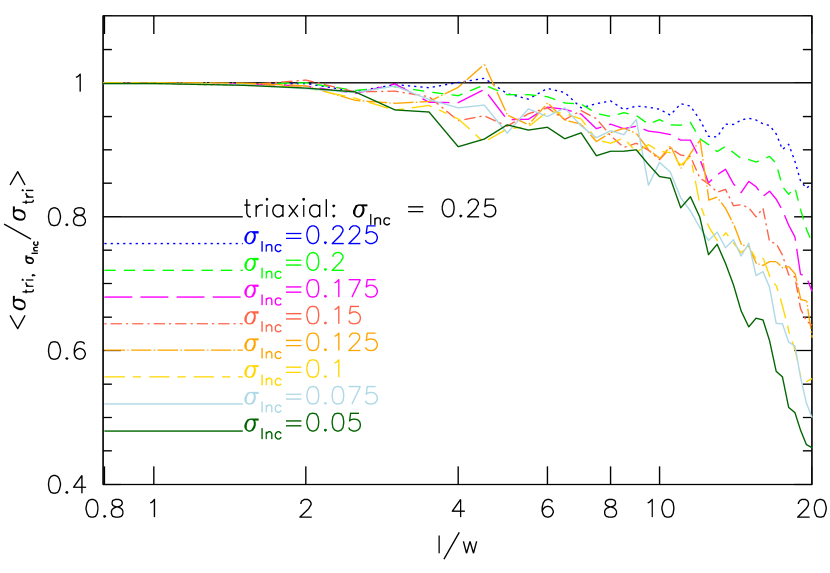
Figure 16: The median ratio of the strong lensing cross section between sample of haloes generated assuming a scatter $\sigma_{\ln c}$ and our fiducial one – where we have assumed $\sigma_{\ln c}=0.25$. Different line types refer to different value of the variance in the log-normal scatter from which we draw the concentration to assign to each host halo in the respective sample.

For each halo sample, we have estimated the standard deviation $\sigma_{\log\sigma}$ for length-to-width ratios $l/w=5$, $7.5$ and $10$. Figure 17 shows the relation between the standard deviation in the strong lensing signal for haloes with $M_{vir}=10^{15}M_{\odot}/h$, $z_{l}=0.25$ and $z_{s}=2$ and the scatter in concentration, rescaled to the scatter for the sample with $\sigma_{\ln c}=0.25$. For the chosen $l/w$ ratios, the correlation is well fit by a straight line. Higher standard deviations in the concentration scatter cause larger strong lensing signals. The dashed lines in all panels show the least-squares fit to the data points,

$$\sigma_{\log\sigma}=a\times\sigma_{\ln c}+b\,,$$ (41)

where we obtain the slopes

$$a=0.714\pm 0.049,\quad\mathrm{for}\quad \sigma_{5}$$

$$a=0.640\pm 0.091,\quad\mathrm{for}\quad \sigma_{7.5}$$

$$a=0.506\pm 0.053,\quad\mathrm{for}\quad \sigma_{10}$$ .

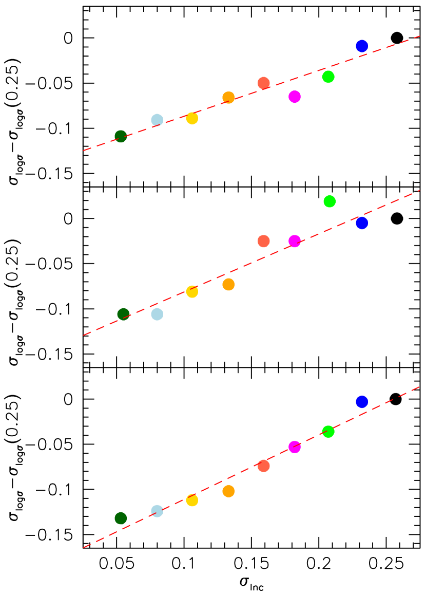
Figure 17: The correlation between the scatter in the strong lensing cross section at three different value of $l/w$ and the scatter in concentration assumed to generate halo samples.

References

- Bartelmann (1996) Bartelmann M., 1996, A&A, 313, 697
- Bartelmann et al. (1998) Bartelmann M., Huss A., Colberg J. M., Jenkins A., Pearce F. R., 1998, A&A, 330, 1
- Bartelmann et al. (2003) Bartelmann M., Meneghetti M., Perrotta F., Baccigalupi C., Moscardini L., 2003, A&A, 409, 449
- Bartelmann & Schneider (2001) Bartelmann M., Schneider P., 2001, Physics Reports, 340, 291
- Blumenthal et al. (1986) Blumenthal G. R., Faber S. M., Flores R., Primack J. R., 1986, ApJ, 301, 27
- Bond et al. (1991) Bond J. R., Cole S., Efstathiou G., Kaiser N., 1991, ApJ, 379, 440
- Bryan & Norman (1998) Bryan G. L., Norman M. L., 1998, ApJ, 495, 80
- Bullock et al. (2001) Bullock J. S., Kolatt T. S., Sigad Y., Somerville R. S., Kravtsov A. V., Klypin A. A., Primack J. R., Dekel A., 2001, MNRAS, 321, 559
- Choi et al. (2007) Choi J.-H., Weinberg M. D., Katz N., 2007, MNRAS, 381, 987
- Croton et al. (2006) Croton D. J., Springel V., White S. D. M., De Lucia G., Frenk C. S., Gao L., Jenkins A., Kauffmann G., Navarro J. F., Yoshida N., 2006, MNRAS, 365, 11
- De Lucia et al. (2004) De Lucia G., Kauffmann G., Springel V., White S. D. M., Lanzoni B., Stoehr F., Tormen G., Yoshida N., 2004, MNRAS, 348, 333
- Dolag et al. (2004) Dolag K., Bartelmann M., Perrotta F., Baccigalupi C., Moscardini L., Meneghetti M., Tormen G., 2004, A&A, 416, 853
- Duffy et al. (2008) Duffy A. R., Schaye J., Kay S. T., Dalla Vecchia C., 2008, MNRAS, 390, L64
- Eke et al. (1996) Eke V. R., Cole S., Frenk C. S., 1996, MNRAS, 282, 263
- Fasano et al. (2010) Fasano G., Bettoni D., Ascaso B., Tormen G., Poggianti B. M., Valentinuzzi T., D’Onofrio M., Fritz J., Moretti A., Omizzolo A., Cava A., Moles M., Dressler A., Couch W. J., Kjærgaard P., Varela J., 2010, MNRAS, 404, 1490
- Fedeli et al. (2006) Fedeli C., Meneghetti M., Bartelmann M., Dolag K., Moscardini L., 2006, A&A, 447, 419
- Fedeli et al. (2010) Fedeli C., Meneghetti M., Gottlöber S., Yepes G., 2010, A&A, 519, A91+
- Gao et al. (2008) Gao L., Navarro J. F., Cole S., Frenk C. S., White S. D. M., Springel V., Jenkins A., Neto A. F., 2008, MNRAS, 387, 536
- Gao et al. (2005) Gao L., Springel V., White S. D. M., 2005, MNRAS, 363, L66
- Gao et al. (2004) Gao L., White S. D. M., Jenkins A., Stoehr F., Springel V., 2004, MNRAS, 355, 819
- Giocoli et al. (2010) Giocoli C., Bartelmann M., Sheth R. K., Cacciato M., 2010, MNRAS, 408, 300
- Giocoli et al. (2007) Giocoli C., Moreno J., Sheth R. K., Tormen G., 2007, MNRAS, 376, 977
- Giocoli et al. (2010a) Giocoli C., Tormen G., Sheth R. K., van den Bosch F. C., 2010a, MNRAS, 404, 502
- Giocoli et al. (2008) Giocoli C., Tormen G., van den Bosch F. C., 2008, MNRAS, 386, 2135
- Hayashi et al. (2003) Hayashi E., Navarro J. F., Taylor J. E., Stadel J., Quinn T., 2003, ApJ, 584, 541
- Hernquist (1990) Hernquist L., 1990, ApJ, 356, 359
- Jing (2000) Jing Y. P., 2000, ApJ, 535, 30
- Jing & Suto (2002) Jing Y. P., Suto Y., 2002, ApJ, 574, 538
- Kazantzidis et al. (2004) Kazantzidis S., Kravtsov A. V., Zentner A. R., Allgood B., Nagai D., Moore B., 2004, ApJ, 611, L73
- Keeton (2001) Keeton C. R., 2001, ApJ, 561, 46
- Keeton (2003) Keeton C. R., 2003, ApJ, 584, 664
- Lacey & Cole (1993) Lacey C., Cole S., 1993, MNRAS, 262, 627
- Mandelbaum et al. (2009) Mandelbaum R., van de Ven G., Keeton C. R., 2009, MNRAS, 398, 635
- Meneghetti et al. (2007b) Meneghetti M., Argazzi R., Pace F., Moscardini L., Dolag K., Bartelmann M., Li G., Oguri M., 2007b, A&A, 461, 25
- Meneghetti et al. (2005a) Meneghetti M., Bartelmann M., Dolag K., Moscardini L., Perrotta F., Baccigalupi C., Tormen G., 2005a, A&A, 442, 413
- Meneghetti et al. (2003) Meneghetti M., Bartelmann M., Moscardini L., 2003, MNRAS, 346, 67
- Meneghetti et al. (2010a) Meneghetti M., Fedeli C., Pace F., Gottlöber S., Yepes G., 2010a, A&A, 519, A90+
- Meneghetti et al. (2011) Meneghetti M., Fedeli C., Zitrin A., Bartelmann M., Broadhurst T., Gottlöber S., Moscardini L., Yepes G., 2011, A&A, 530, A17+
- Meneghetti et al. (2005b) Meneghetti M., Jain B., Bartelmann M., Dolag K., 2005b, MNRAS, 362, 1301
- Meneghetti et al. (2010b) Meneghetti M., Rasia E., Merten J., Bellagamba F., Ettori S., Mazzotta P., Dolag K., Marri S., 2010b, A&A, 514, A93+
- Metcalf & Madau (2001) Metcalf R. B., Madau P., 2001, MNRAS, 563, 9
- Moore et al. (1999) Moore B., Ghigna S., Governato F., Lake G., Quinn T., Stadel J., Tozzi P., 1999, ApJ, 524, L19
- Navarro et al. (1996) Navarro J. F., Frenk C. S., White S. D. M., 1996, ApJ, 462, 563
- Neto et al. (2007) Neto A. F., Gao L., Bett P., Cole S., Navarro J. F., Frenk C. S., White S. D. M., Springel V., Jenkins A., 2007, MNRAS, 381, 1450
- Newman et al. (2011) Newman A. B., Treu T., Ellis R. S., Sand D. J., 2011, ApJ, 728, L39+
- Newman et al. (2009) Newman A. B., Treu T., Ellis R. S., Sand D. J., Richard J., Marshall P. J., Capak P., Miyazaki S., 2009, ApJ, 706, 1078
- Oguri et al. (2009) Oguri M., Hennawi J. F., Gladders M. D., Dahle H., Natarajan P., Dalal N., Koester B. P., Sharon K., Bayliss M., 2009, ApJ, 699, 1038
- Oguri et al. (2003) Oguri M., Lee J., Suto Y., 2003, ApJ, 599, 7
- Oguri et al. (2005) Oguri M., Takada M., Umetsu K., Broadhurst T., 2005, ApJ, 632, 841
- Press & Schechter (1974) Press W. H., Schechter P., 1974, ApJ, 187, 425
- Puchwein et al. (2005) Puchwein E., Bartelmann M., Dolag K., Meneghetti M., 2005, A&A, 442, 405
- Refregier et al. (2010) Refregier A., Amara A., Kitching T. D., Rassat A., Scaramella R., Weller J., Euclid Imaging Consortium f. t., 2010, ArXiv e-prints
- Richard et al. (2010) Richard J., Smith G. P., Kneib J.-P., Ellis R. S., Sanderson A. J. R., Pei L., Targett T. A., Sand D. J., Swinbank A. M., Dannerbauer H., Mazzotta P., Limousin M., Egami E., Jullo E., Hamilton-Morris V., Moran S. M., 2010, MNRAS, 404, 325
- Sand et al. (2004) Sand D. J., Treu T., Smith G. P., Ellis R. S., 2004, ApJ, 604, 88
- Shaw et al. (2007) Shaw L. D., Weller J., Ostriker J. P., Bode P., 2007, ApJ, 659, 1082
- Sheth & Tormen (1999) Sheth R. K., Tormen G., 1999, MNRAS, 308, 119
- Sheth & Tormen (2002) Sheth R. K., Tormen G., 2002, MNRAS, 329, 61
- Sheth & Tormen (2004a) Sheth R. K., Tormen G., 2004a, MNRAS, 349, 1464
- Sheth & Tormen (2004b) Sheth R. K., Tormen G., 2004b, MNRAS, 350, 1385
- Smith & Taylor (2008) Smith G. P., Taylor J. E., 2008, ApJ, 682, L73
- Springel et al. (2001b) Springel V., White S. D. M., Tormen G., Kauffmann G., 2001b, MNRAS, 328, 726
- Tormen et al. (1998) Tormen G., Diaferio A., Syer D., 1998, MNRAS, 299, 728
- Torri et al. (2004) Torri E., Meneghetti M., Bartelmann M., Moscardini L., Rasia E., Tormen G., 2004, MNRAS, 349, 476
- Umetsu et al. (2011) Umetsu K., Broadhurst T., Zitrin A., Medezinski E., Coe D., Postman M., 2011, ArXiv e-prints
- van de Ven et al. (2009) van de Ven G., Mandelbaum R., Keeton C. R., 2009, MNRAS, 398, 607
- van den Bosch et al. (2004) van den Bosch F. C., Norberg P., Mo H. J., Yang X., 2004, MNRAS, 352, 1302
- van den Bosch et al. (2005) van den Bosch F. C., Tormen G., Giocoli C., 2005, MNRAS, 359, 1029
- Wang et al. (2006) Wang L., Li C., Kauffmann G., De Lucia G., 2006, MNRAS, 371, 537
- Wechsler et al. (2002) Wechsler R. H., Bullock J. S., Primack J. R., Kravtsov A. V., Dekel A., 2002, ApJ, 568, 52
- Wu et al. (1998) Wu X.-P., Fang L.-Z., Xu W., 1998, A&A, 338, 813
- Zhao et al. (2009) Zhao D. H., Jing Y. P., Mo H. J., Bnörner G., 2009, ApJ, 707, 354
- Zhao et al. (2003b) Zhao D. H., Jing Y. P., Mo H. J., Börner G., 2003b, ApJ, 597, L9
- Zhao et al. (2003a) Zhao D. H., Mo H. J., Jing Y. P., Börner G., 2003a, MNRAS, 339, 12
- Zitrin et al. (2011a) Zitrin A., Broadhurst T., Barkana R., Rephaeli Y., Benítez N., 2011a, MNRAS, 410, 1939
- Zitrin et al. (2011c) Zitrin A., Broadhurst T., Bartelmann M., Rephaeli Y., Oguri M., Benítez N., Hao J., Umetsu K., 2011c, ArXiv e-prints