Numerical solution for a non-Fickian diffusion in a periodic potential

Abstract

Numerical solutions of a non-Fickian diffusion equation belonging to a hyperbolic type are presented in one space dimension. The Brownian particle modelled by this diffusion equation is subjected to a symmetric periodic potential whose spatial shape can be varied by a single parameter. We consider a numerical method which consists of applying Laplace transform in time; we then obtain an elliptic diffusion equation which is discretized using a finite difference method. We analyze some aspects of the convergence of the method. Numerical results for particle density, flux and mean-square-displacement (covering both inertial and diffusive regimes) are presented.

keywords: numerical methods, Laplace transform, telegraph equation, periodic

potential, non-Fickian diffusion

1 Introduction

In this paper we shall present numerical solutions of a non-Fickian diffusion equation in the presence of a symmetric periodic potential in one space dimension. Let us briefly recall that the Fickian diffusion equation in the presence of a potential $V(\xi)$ reads

$$\frac{\partial n}{\partial\tau}(\xi,\tau)=D\frac{\partial^{2}n}{\partial\xi^{2}}(\xi,\tau)+\frac{1}{m\gamma}\frac{\partial}{\partial\xi}\left[\frac{dV}{d\xi}(\xi)n(\xi,\tau)\right],$$ (1)

where $\gamma$ is a friction parameter and $D=k_{B}T/m\gamma$ is the diffusion coefficient, $m$ being the mass of the Brownian particle whose overdamped (diffusive) dynamics is well described by (1), $k_{B}$ is the Boltzmann’s constant and $T$ the temperature of the fluid.

The equation of our study is

$$\frac{1}{\gamma}\frac{\partial^{2}n}{\partial\tau^{2}}(\xi,\tau)+\frac{\partial n}{\partial\tau}(\xi,\tau)=D\frac{\partial^{2}n}{\partial\xi^{2}}(\xi,\tau)+\frac{1}{m\gamma}\frac{\partial}{\partial\xi}\left[\frac{dV}{d\xi}(\xi)n(\xi,\tau)\right].$$ (2)

Both equations, (1) and (2) can be derived from an underlying kinetic equation e.g. the phase-space Kramers equation [8]

$$\frac{\partial f}{\partial\tau}+\frac{p}{m}\frac{\partial f}{\partial\xi}-\frac{dV}{d\xi}\frac{\partial f}{\partial p}=\gamma\frac{\partial}{\partial p}(pf)+mk_{B}T\gamma\frac{\partial^{2}f}{\partial p^{2}},$$ (3)

where $f(\xi,p,\tau)$ is the probability density function for the position component $\xi$ and momentum component $p$ of the Brownian particle.

Equation (2) in the absence of a potential field is sometimes referred to the telegrapher equation although we shall call it a non-Fickian diffusion equation. We refer to [8] for a derivation of (2) from (3). It may be noted that for times larger than $1/\gamma$ , the first term on the left hand side of (2) can be neglected and the Fickian regime is regained. Equation (1) in the absence of a potential field leads to the well known result for the mean square displacement [10]

$$<\xi^{2}(\tau)>=2D\tau.$$ (4)

In the presence of a flexible symmetric potential, it was shown in [8] that $<\xi^{2}(\tau)>$ does not necessarily behave linearly with time. Equation (2) retains some short time inertial behaviour of a Brownian particle and at long time results in a diffusive behaviour. The velocity $v=d\xi/d\tau$ of a Brownian particle is not well defined in the diffusive regime for which (1) is applicable. Since (2) is applicable in an inertial regime, the velocity can be calculated with (2). Quite recently the instantaneous velocity of a Brownian particle has been experimentally investigated [11, 12, 17]. This provides an additional motivation for studying (2). There is also a recent paper [4] which models transport of ions in insulating media through a non-Fickian diffusion equation of the type discussed in our work. In [4] the non-Fickian diffusion equation is referred to as a hyperbolic diffusion equation .

To solve our problem we consider a numerical method based on space discretization and time Laplace transform. The latter is suitable for long times and also for solutions that are not necessarily smooth in time. It may be noted that iterative methods in time, including implicit methods such as the Crank- Nicolson [7], which allows a choice of large time steps, usually take too long to compute the solution.

The paper is organized as follows. In section 2 we present the model problem in dimensionless variables. In section 3 we describe a numerical method based on the time Laplace transform which is suitable for long time integration and also for solutions which are not very smooth. In section 4 the convergence properties of the algorithm are studied. In section 5 we present the behaviour of the solution to the non-Fickian diffusion equation, the flux and the mean square displacement. We conclude the paper, in section 6, with a summary and outlook.

2 The model and physical quantities

In our studies we consider three quantities of physical interest. These are the particle density  $n(\xi,\tau)$,  the  current  density  (flux)  $j(\xi,\tau)$ and  the  mean square  displacement
$<\xi^{2}(\tau)>$. The current density is not normally studied. However, since we are dealing with a non-Fickian diffusion equation we have decided to consider $j(\xi,\tau)$ as well. For the Fickian case and in the absence of any potential, $j(\xi,\tau)$ is related to $n(\xi,\tau)$ through $j=-D(\partial n/\partial\xi)$. This is not so in the non-Fickian case for which the relation between $j(\xi,\tau)$ and $n(\xi,\tau)$ is more involved.

Let us consider the non-Fickian diffusion equations for particle density and the flux

$$\frac{1}{\gamma}\frac{\partial^{2}n}{\partial\tau^{2}}+\frac{\partial n}{\partial\tau} = -\frac{1}{m\gamma}\frac{\partial}{\partial\xi}(Pn)+D\frac{\partial^{2}n}{\partial\xi^{2}},$$ (5)

$$j+\frac{1}{\gamma}\frac{\partial j}{\partial\tau} = -D\frac{\partial n}{\partial\xi}-\frac{1}{m\gamma}Pn,$$ (6)

with $n(\xi,\tau)$ as the density of the Brownian particles. $P$ is the force acting on the particle due to the potential field $V$, i.e.

$$P=-\frac{dV}{d\xi}.$$

We consider a symmetric periodic potential field, as previously studied in [5], [8] and [13]. It reads

$$V(\xi;\alpha)=\frac{1}{J_{0}(\mathbb{i}\alpha)}e^{\alpha\cos{\xi}}-1,$$ (7)

where $J_{0}$ is the Bessel function of the first kind and zero order and $\mathbb{i}$ is the imaginary number. In order to illustrate the flexible form of this single-parameter potential we have plotted, Figure 1, the potential (7), for two values of the parameter, $\alpha=1$ and $\alpha=16$.

  

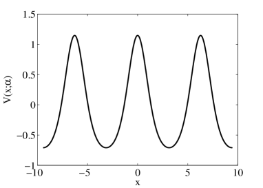
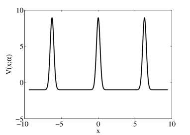
Figure 1: Potential field $V(x;\alpha)$. Left figure: $\alpha=1$; Right figure: $\alpha=16$.

Our model consists of equations (5) and (6), and the potential field $V(\xi;\alpha)$ given by (7). For later purpose we introduce the following dimensionless parameters

$$n=\frac{n}{n_{0}},\qquad x=\frac{\xi}{\sqrt{D/\gamma}},\qquad t=\tau\gamma,$$ (8)

where $n_{0}$ is a reference particle density (concentration). The dimensionless forms of (2) and (6) can be written as

$$\frac{\partial^{2}n}{\partial t^{2}}+\frac{\partial n}{\partial t} = -\frac{\partial}{\partial x}(Pn)+\frac{\partial^{2}n}{\partial x^{2}},$$ (9)

$$j+\frac{\partial j}{\partial t} = -\sqrt{D}\sqrt{\gamma}\frac{\partial n}{\partial x}+\gamma P(x)n,$$ (10)

with

$$P(x)=-\frac{1}{m\sqrt{D\gamma^{3}}}\frac{dV}{dx}.$$ (11)

3 Numerical method

We consider equations (9) and (10) with the following initial conditions

$$n\left(x,0\right) = \frac{1}{L\sqrt{\pi}}e^{-x^{2}/L^{2}},{\ \ \ \ }\frac{\partial n}{\partial t}\left(x,0\right)=0,$$ (12)

$$j\left(x,0\right) = \frac{1}{L\sqrt{\pi}}e^{-x^{2}/L^{2}}\left(\frac{\sqrt{D}\sqrt{\gamma}}{L^{2}}2x+\gamma P(x)\right),$$ (13)

where

$$P(x)=-\frac{1}{m\sqrt{D\gamma^{3}}}\frac{dV}{dx},\qquad V(x;\alpha)=\frac{1}{J_{0}(\bf{i}\alpha)}e^{\alpha\cos{x}}-1.$$

The boundary conditions are given by

$$\lim_{x\rightarrow\infty}n(x,t)=0,\quad\lim_{x\rightarrow-\infty}n(x,t)=0$$ (14)

and

$$\lim_{x\rightarrow\infty}j(x,t)=0,\quad\lim_{x\rightarrow-\infty}j(x,t)=0.$$ (15)

In this section we describe a numerical method to solve the problem (9)–(10). Our approach can be separated in three steps. First, we apply the Laplace transform to (9)–(10) in order to remove the time dependent terms and we obtain an ordinary differential equation in $x$ that also depends on the Laplace transform parameter $s$. Secondly, we solve the ordinary differential equation obtained using a finite difference scheme. Lastly, using a numerical inverse Laplace transform algorithm we obtain the final approximate solution.

3.1 Spatial discretization

Our numerical method is facilitated if we apply time Laplace transform to equation (9) and obtain the ordinary differential equation

$$\frac{d^{2}\widetilde{n}}{dx^{2}}-\lambda_{s}\widetilde{n}-\frac{d}{dx}\left(P\widetilde{n}\right)=-(1+s)n(x,0),$$ (16)

where $\lambda_{s}=s^{2}+s$, $s$ is a complex variable and $\widetilde{n}$ is the Laplace transform of $n$ defined by

$$\widetilde{n}(x,s)=\int_{0}^{\infty}{\rm e}^{-st}n(x,t)dt.$$

Now, assume we have a space discretization $x_{i}=a+i\Delta x,\ i=0,\dots,N$. Let $\widetilde{\eta}_{i}(s),\ i=0,\dots,N$ represent the approximation of $\widetilde{n}\left(x_{i},s\right)$ in the Laplace transform domain. The outflow boundary is such that $\tilde{\eta}_{N}(s)=0$, for all $s$ and $N$ sufficiently large, which is according to the physical boundary condition.

To derive the numerical method we consider central differences to approximate the first derivative and the second derivative of equation (16). We obtain, for a fixed $s$, the finite difference scheme given by

$$\frac{\widetilde{\eta}_{i-1}(s)-2\widetilde{\eta}_{i}(s)+\widetilde{\eta}_{i+1}(s)}{\Delta x^{2}}-\lambda_{s}\widetilde{\eta}_{i}(s)-\frac{P_{i+1}\widetilde{\eta}_{i+1}(s)-P_{i-1}\widetilde{\eta}_{i-1}(s)}{2\Delta x}=-(1+s)n(x_{i},0),$$ (17)

for $i=1,\ldots,N-1$, where $P_{i}=P(x_{i})$.

Therefore, we obtain the linear system

$$K\left(s\right)\widetilde{\bf\eta}\left(s\right)=\widetilde{b}\left(s\right),$$ (18)

where $K(s)=[K_{i,j}(s)]$ is a band matrix of size $N-1\times N-1$ with bandwidth three and $\widetilde{\bf\eta}\left(s\right)=[\widetilde{\eta}_{1}\left(s\right),\ldots,\widetilde{\eta}_{N-1}\left(s\right)]^{T}$. The matrix $K(s)$ has entries of the form

$$K_{i,i-1}(s) = \frac{1}{\Delta x^{2}}+\frac{P_{i-1}}{2\Delta x},$$

$$K_{i,i}(s) = -\frac{2}{\Delta x^{2}}-\lambda_{s},$$

$$K_{i,i+1}(s) = \frac{1}{\Delta x^{2}}-\frac{P_{i+1}}{2\Delta x},$$ (19)

and $\widetilde{b}\left(s\right)$ contains boundary conditions, being represented by

$$\widetilde{b}\left(s\right)=\left[\begin{array}[]{c}-(1+s)n(x_{1},0)\\ -(1+s)n(x_{2},0)\\ \vdots\\ -(1+s)n(x_{N-2},0)\\ -(1+s)n(x_{N-1},0)\\ \end{array}\right]+\left[\begin{array}[]{c}-K_{1,0}(s)\widetilde{\eta}_{0}(s)\\ 0\\ \vdots\\ 0\\ -K_{N-1,N}(s)\widetilde{\eta}_{N}(s)\\ \end{array}\right].$$ (20)

To compute the flux, we apply the Laplace transform to equation (10), that is,

$$(1+s)\widetilde{j}=-\sqrt{D}\sqrt{\gamma}\frac{d\widetilde{n}}{dx}+\gamma P(x)\widetilde{n}+j(x,0),$$ (21)

where $\widetilde{j}$ is the Laplace transform of the flux $j$. The last step is to determine an approximate solution $\eta_{i}\left(t\right)$ and $j_{i}(t)$ of $n(x_{i},t)$ and $j(x_{i},t)$ respectively, which is obtained from $\widetilde{\eta}_{i}\left(s\right)$ and $\widetilde{j}_{i}\left(s\right)$ by using a Laplace inversion numerical method.

3.2 Laplace transform inversion

In this section, we determine an approximate solution $\eta_{i}\left(t\right)$ from $\widetilde{\eta}_{i}\left(s\right)$ by using a Laplace inversion numerical method. For the sake of clarity we omit the index $i$, denoting $\widetilde{\eta}_{i}\left(s\right)$ by $\widetilde{\eta}\left(s\right)$.

A formally exact inverse Laplace transform of $\widetilde{\eta}\left(s\right)$ into $\overline{\eta}\left(t\right)$ is given through the Bromwich integral [14]

$$\overline{\eta}\left(t\right)=\frac{1}{2\pi{\bf i}}\int_{\beta-{\bf i}\infty}^{\beta+{\bf i}\infty}{\rm e}^{st}\widetilde{\eta}\left(s\right)ds,$$ (22)

where $\beta$ is such that the contour of integration is to the right-hand side of any singularity of $\widetilde{\eta}\left(s\right)$. However, for a numerical evaluation the above integral is first transformed to an equivalent form

$$\overline{\eta}\left(t\right)=\frac{1}{\pi}{\rm e}^{\beta t}\int_{0}^{\infty}\mbox{Re}\left\{\widetilde{\eta}\left(s\right){\rm e}^{{\bf{i}}\omega t}\right\}\hskip 0.72229ptd\omega,$$ (23)

where $s=\beta+{\bf{i}}\omega$ [1, 14, 15]. The integral is now evaluated through the trapezoidal rule [1, 6], with step size $\pi/T$, and we obtain

$$\overline{\eta}(t)=\frac{1}{T}{\rm e}^{\beta t}\left[\frac{\widetilde{\eta}\left(\beta\right)}{2}+\sum_{k=1}^{\infty}\mbox{Re}\left\{\widetilde{\eta}\left(\beta+\frac{{\bf{i}}k\pi}{T}\right){\rm e}^{\frac{{\bf{i}}k\pi t}{T}}\right\}\right]-E_{T},$$ (24)

for $0<t<2T$ and where $E_{T}$ is the discretization error. It is known that the infinite series in this equation converges very slowly. To accelerate the convergence, we apply the quotient-difference algorithm, proposed in [2], and also used in [15], to calculate the series in (24) by the rational approximation in the form of a continued fraction. Under some conditions we can always associate a continued fraction to a given power series.

We denote $v\left(z\right)$ the continued fraction

$$v\left(z\right)=d_{0}/\left(1+d_{1}z/\left(1+d_{2}z/\left(1+\cdots\right)\right)\right)$$ (25)

associated to the power series in (24). For $z={\rm e}^{{\bf{i}}\pi t/T}$,

$$v\left(z\right)=\frac{\widetilde{\eta}\left(\beta\right)}{2}+\sum_{k=1}^{\infty}\widetilde{\eta}\left(\beta+\frac{{\bf{i}}k\pi}{T}\right)z^{k},$$ (26)

and the coefficients $d_{i}$’s of (25) are obtained by recurrence relations from the coefficients $\widetilde{\eta}\left(\beta+\frac{{\bf{i}}k\pi}{T}\right)$.

Let the $M$-th partial fraction be denoted by $v(z,M)$. Therefore

$$v\left(z\right)=v\left(z,M\right)+E_{F}^{M},$$

where $E_{F}^{M}$ is the truncation error. Then

$$\overline{\eta}\left(t\right)=\frac{1}{T}{\rm e}^{\beta t}\mbox{Re}\left\{v\left(z,M\right)+E_{F}^{M}\right\}-E_{T}.$$

The approximation for $\overline{\eta}\left(t\right)$ is denoted by $\eta(t)$ and given by

$$\eta\left(t\right)=\frac{1}{T}{\rm e}^{\beta t}\mbox{Re}\left\{v\left(z,M\right)\right\}\mbox{.}$$

4 Convergence of the numerical method

In this section we discuss the convergence of the numerical method chosen to compute an approximate solution to equation (9). Let us denote by $\widetilde{E}_{S}$ the error associated to the spatial discretization, that is,

$$\widetilde{n}(x_{i},s)=\widetilde{\eta}_{i}(s)+\widetilde{E}_{S}(x_{i},s).$$ (27)

The next errors come from the numerical inversion of Laplace transform, where the Laplace inverse transform of $\widetilde{\eta}_{i}(s)$ is, as described in the previous section, the solution

$$\overline{\eta}_{i}\left(t\right)=\frac{1}{T}{\rm e}^{\beta t}\mbox{Re}\left\{v\left(z,M_{i}\right)+E_{F}^{M}(x_{i},t)\right\}-E_{T}(x_{i},t),$$ (28)

where $E_{T}$ is the error associated with the trapezoidal approximation and $E_{F}^{M}$ is the truncation error associated to the continued fraction. Note that for each $x_{i}$ the algorithm chooses a $M_{i}$ and therefore for each $x_{i}$ we have a different value of the approximation of the continued fraction, $v\left(z,M_{i}\right)$. Therefore from (27)–(28) we have

$${n}(x_{i},t)=\frac{1}{T}{\rm e}^{\beta t}\mbox{Re}\left\{v\left(z,M_{i}\right)+E_{F}^{M}(x_{i},t)\right\}-E_{T}(x_{i},t)+{E}_{S}(x_{i},t),$$

where ${E}_{S}(x_{i},t)$ is the inverse Laplace transform of the error $\widetilde{E}_{S}(x_{i},s)$.

Approximation errors $E_{T}$ and $E_{F}$

The error $E_{T}$ that comes from the integral approximation using the trapezoidal rule, according to Crump [6], is

$$E_{T}=\sum_{n=1}^{\infty}{\rm e}^{-2n\beta T}n(x_{i},2nT+t).$$

Assume now that our function is bounded such as $|n(x_{i},t)|\leq{\rm e}^{\sigma t}$, for all $x_{i}$. Therefore the error can be bounded by

$$E_{T}\leq{\rm e}^{\sigma t}\sum_{n=1}^{\infty}{\rm e}^{-2nT(\beta-\sigma)}=\frac{{\rm e}^{\sigma t}}{{\rm e}^{2T(\beta-\sigma)}-1},\quad 0<t<2T.$$

It follows that by choosing $\beta$ sufficiently larger than $\sigma$, we can make $E_{T}$ as small as desired. For practical purposes and in order to choose a convenient $\beta$ we use the inequality which bounds the error

$$E_{T}\leq{\rm e}^{\sigma t-2T(\beta-\sigma)}.$$

If we want to have the bound $E_{T}\leq b_{T}$ then by applying the logarithm in both sides of the previous inequality we have

$$\beta\geq\sigma\frac{2T+t}{2T}-\frac{1}{2T}\ln\left({b_{T}}\right).$$

Assuming $\sigma\geq 0$ we can write

$$\beta\geq\sigma-\frac{\ln\left(b_{T}\right)}{2T}.$$

In our example we consider $\sigma=0$. In practice the trapezoidal error $E_{T}$ is controlled by the parameter $\beta$ we choose.

The second error, $E_{F}^{M}$, comes from the approximation of the continued fraction given by (26). This error is controlled by imposing a tolerance $TOL$ such as

$$\left|v\left(z,M\right)-v\left(z,M-1\right)\right|<TOL,$$

in order to get the approximation $\eta_{i}(t)$ given by

$$\eta_{i}(t)=\frac{1}{T}{\rm e}^{\beta t}\mbox{Re}\{v\left(z,M_{i}\right)\},$$

where $M_{i}$ changes according to which $x_{i}$ we are considering.

  

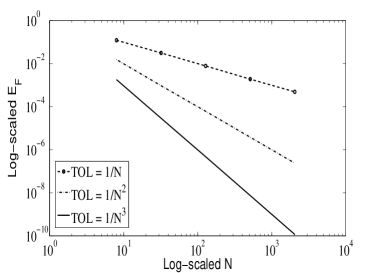
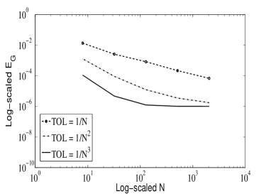
Figure 2: Error $E_{F}$ and $E_{G}$ for $P=2$, $t=1$, $0\leq x\leq 12$ and $\beta=-\ln(10^{-6})/2T$ and different values of $TOL$. The global error is controlled by the parameter $\beta$.

  

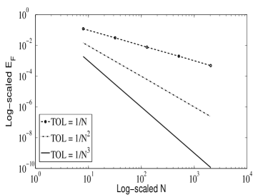
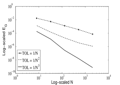
Figure 3: Error $E_{F}$ and $E_{G}$ for $P=2$, $t=1$, $0\leq x\leq 12$ and $\beta=-\ln(10^{-10})/2T$ and different values of $TOL$. The parameter $\beta$ is chosen such that the global error is not affected.

In order to understand better how to control the trapezoidal error with the parameter $\beta$ and how the tolerance $TOL$ affects the error, we present a test example which is an analytically exactly solvable model. We assume $P$ constant and Fickian diffusion

$$\frac{\partial n}{\partial t}=-P\frac{\partial n}{\partial x}+D\frac{\partial^{2}n}{\partial x^{2}},\mbox{ \ }x\in\left]0,\infty\right[,t>0.$$ (29)

The initial condition is $n(x,0)=0$, and the boundary conditions are

$$n(0,t)=N_{0},\qquad n(\infty,t)=0.$$ (30)

It will be noted that we are now considering a semi-infinite geometry. We note the difference between this test case and our original unbound problem. We choose this test example for two reasons: Firstly, equation (29) can be analytically exactly solved by first applying the time-Laplace transform and then through the inverse Laplace transform. Secondly, this example is chosen to compare the convergence aspects of the Laplace inversion algorithm without spatial discretization.

If we apply the Laplace transform to this problem we obtain

$$\widetilde{n}(x,s)=N_{0}\frac{1}{s}{\rm e}^{P/2D-x\sqrt{(P/2D)^{2}+s}}.$$ (31)

The analytical solution is given by

$$n\left(x,t\right)=\frac{N_{0}}{2}\left(\mathrm{erfc}\left[\frac{x-Pt}{2\sqrt{Dt}}\right]+{\rm e}^{{Px}/{D}}\mathrm{erfc}\left[\frac{x+Pt}{2\sqrt{Dt}}\right]\right).$$ (32)

In Figures 2 and  3, for $P=2$, $t=1$ and $0\leq x\leq 12$, we plot the following errors,

$$E_{F}=\max_{1\leq i\leq N-1}|v(z,M_{i})-v(z,M_{i}-1)|$$ (33)

and

$$E_{G}=||n(x_{i},t)-\eta_{i}(t)||_{\infty},$$ (34)

where $||\cdot||_{\infty}$ is the infinity norm. We choose the interval $0\leq x\leq 12$ in order to avoid the influence of the right numerical boundary condition in the numerical computations, that in this case is $n(12,t)=0$.

The error $E_{F}$ is related with the error $E_{F}^{M}$ since we control $E_{F}^{M}$ by controlling $E_{F}$ with the tolerance $TOL$. Figures 2 and 3 show how the parameter $\beta$, given by $\beta=-\ln(10^{-6})/2T$ in Figure 2 and $\beta=-\ln(10^{-10})/2T$ in Figure 3, affects the global convergence. Note that in Figure 2 the precision does not go further than $10^{-6}$. The global error of Figure 2 and Figure 3 is not affected by the spatial error $E_{S}$ since we apply the Laplace inversion algorithm directly in (31).

  

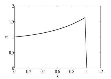
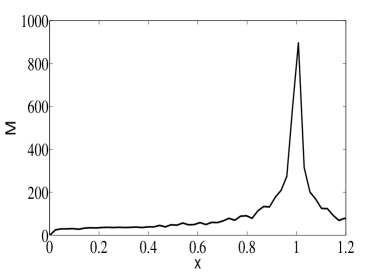
Figure 4: Number of iterations $M$ for $P=2$, $t=1$ and $TOL=1/N^{2}$. Left figure: Approximate solution; Right figure: Number of iterations for each $x_{i}$.

The Laplace inversion algorithm approximates the value of the infinite series using a truncated continued fraction and this truncation is done by choosing an $M_{i}$ for each $x_{i}$. This $M_{i}$ is chosen according to which value of the tolerance $TOL$ we consider. We show in Figure  4 the variations of $M_{i}$ and it is clear the algorithm concentrates the high values of $M$ in the region that presents steep gradients.

Spatial discretization error $\widetilde{E}_{S}(x_{i},s)$

We now turn to the discretization error $\widetilde{E}_{S}(x_{i},s)$, defined in (27) (our main problem), and prove that the method has truncation error of second order. Let us denote the differential operator $L$ given by

$$L\widetilde{n}=\frac{d^{2}\widetilde{n}}{dx^{2}}-\lambda_{s}\widetilde{n}-\frac{d}{dx}\left(P\widetilde{n}\right).$$

We also denote by $L_{\pi}$, the operator associated with the spatial discretization, given by

$$L_{\pi}\widetilde{n}(x_{i},s)=\frac{\widetilde{n}_{i-1}(s)-2\widetilde{n}_{i}(s)+\widetilde{n}_{i+1}(s)}{\Delta x^{2}}-\lambda_{s}\widetilde{n}_{i}(s)-\frac{P_{i+1}\widetilde{n}_{i+1}(s)-P_{i-1}\widetilde{n}_{i-1}(s)}{2\Delta x},$$

where $\widetilde{n}_{i}(s)$ denotes the exact solution at $\widetilde{n}(x_{i},s)$. The local truncation error is given by

$$T_{e}(x_{i},s)=L_{\pi}\widetilde{n}(x_{i},s)-L\widetilde{n}(x_{i},s).$$

For a fixed $s$, we make a Taylor expansions of the functions $\widetilde{n}$ and $P$ around the point $x_{i}$. We obtain, for a sufficiently smooth $\widetilde{n}$,

$$K_{i,i-1}(s)\widetilde{n}_{i-1}(s)+K_{i,i}(s)\widetilde{n}_{i}(s)+K_{i,i+1}(s)\widetilde{n}_{i+1}(s)+(1+s)n(x_{i},0)$$

$$= \frac{d^{2}\widetilde{n}_{i}}{dx^{2}}(s)-\lambda_{s}\widetilde{n}_{i}(s)-\frac{d}{dx}(P\widetilde{n})_{i}(s)+(1+s)n(x_{i},0)$$

$$+\left[-\frac{1}{6}P^{\prime\prime\prime}_{i}\widetilde{n}_{i}(s)-\frac{1}{2}P^{\prime\prime}_{i}\frac{d\widetilde{n}_{i}}{dx}(s)-\frac{1}{2}P^{\prime}_{i}\frac{d^{2}\widetilde{n}_{i}}{dx^{2}}(s)-\frac{1}{6}P_{i}\frac{d^{3}\widetilde{n}_{i}}{dx^{3}}(s)+\frac{1}{12}\frac{d^{4}\widetilde{n}_{i}}{dx^{4}}(s)\right]\Delta x^{2}$$

$$+\mathcal{O}(\Delta x^{3}),$$

where $P^{\prime},P^{\prime\prime},P^{\prime\prime\prime}$ denotes the derivatives of $P$ (unlike in the previous test example $P$ is now not a constant). From this result we can conclude that, for $\widetilde{n}(.,s)\in C^{4}(\mathbb{R})$, we have

$$||T_{e}||_{\infty}=\max_{2\leq i\leq N}|T_{e}(x_{i},s)|\leq c\Delta x^{2}.$$

By denoting $\widetilde{E}_{i}=\widetilde{E}_{S}(x_{i},s),\ i=1,\dots,N-1$ we have

$$L_{\pi}\widetilde{E}_{i}=T_{e}(x_{i},s),$$

that is,

$$K(s)\widetilde{E}(s)=T_{e}(s).$$

If $||K^{-1}(s)||_{\infty}\leq C$ then $|\widetilde{E}_{i}|\leq C||T_{e}||_{\infty}$. Since the matrix $K(s)$ is not an M-matrix [18, 19], it is not easy to prove analytically the inverse of $K(s)$ is bounded. This difficulty is related to the set of values of the parameter $\lambda_{s}$, given by

$$\lambda_{s}=s^{2}+s=\beta^{2}+\beta-\omega^{2}+\mathbb{i}\omega(2\beta+1),\qquad\omega=\frac{k\pi}{T},\quad k=1,\dots,r,$$

where $r$ defines the set of values in the Laplace domain, since for $\omega^{2}>\beta^{2}+\beta$ the complex $\lambda_{s}$ has negative real part. However, it is easy to see numerically that for a fixed $T$, where $T$ defines the stepsize of the trapezoidal rule used to approximate the integral (23), as we refine the space step, the value $||K^{-1}(s)||_{\infty}$ does not change significantly. We also observe that $||K^{-1}(s)||_{\infty}$ is larger for values of $|s|$ close to zero, indicating that the convergence can be slower for these values, as can be observed in Figure 5.

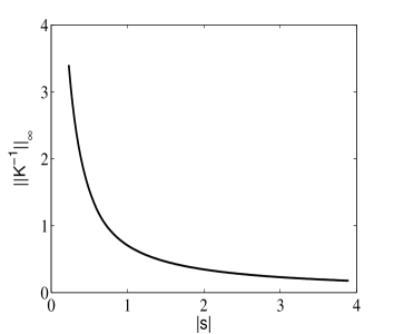
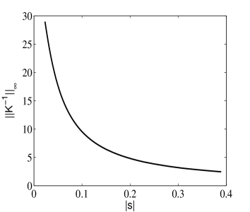
Figure 5: Infinity norm of the matrix $K^{-1}(s)$ for $N=1000$. We have considered $P(x)$ with $\alpha=1$. Left figure: $T=80$; Right figure: $T=800$.

Additionally we observe that we have a similar phenomenom to the so-called pollution effect [3] observed for the Helmholtz equation and high wavenumbers where the discretization space step has to be sufficiently refined to avoid numerical dispersion. Also in this context it is observed that if we have a complex number as a coefficient in the equation, which is our case with $\lambda_{s}$, the imaginary part acts as an absorption parameter, which seems to allow us to control better the solution, decreasing the solution magnitude [9]. Following what is reported in literature [3, 16], a natural rule observed for an adjustment of the space step is to force some relation between $T$ and the $\Delta x$. In our numerical experiments in order to retain accuracy we have considered

$$\frac{t}{T}\Delta x\leq\frac{2}{100}.$$ (35)

Numerical tests: Order of convergence of the numerical method

In order to illustrate the behaviour of the numerical method, we consider two test problems. First, we consider the Fickian problem (29)–(30), which exact solution is given by (32). In Table 1 we show the global error (34), for $P=2$, $t=1$ and different values of the space step. The value of $T=20$ was considered in order to verify (35). These results confirm that the convergence is of second order. We can obtain similar results for other values of $P$.

$\Delta x$	Error	Rate
$10/32$	$0.4000\times 10^{-2}$
$10/128$	$0.2596\times 10^{-3}$	$2.0$
$10/512$	$0.1625\times 10^{-4}$	$2.0$
$10/2048$	$0.1016\times 10^{-5}$	$2.0$

Table 1: Fickian case: Global error (34) for $P=2$, $t=1$, $0\leq x\leq 10$, $TOL=1/N^{3}$, $\beta=-\ln(10^{-16})/2T$, $T=20$.

We now consider a non-Fickian problem given by the telegraph equation,

$$\frac{\partial n}{\partial t}+\frac{\partial^{2}n}{\partial t^{2}}=D\frac{\partial^{2}n}{\partial x^{2}},\mbox{ \ }x\in\left]0,2\pi\right[,t>0,$$ (36)

with initial conditions

$$n(x,0)=\sin(\frac{x}{2}),\qquad\frac{\partial n}{\partial t}(x,0)=-\frac{1}{2}\sin(\frac{x}{2}),$$ (37)

and boundary conditions

$$n(0,t)=0,\qquad n(2\pi,t)=0.$$ (38)

We can easily obtain the analytical solution given by

$$n\left(x,t\right)=e^{-\frac{t}{2}}\sin(\frac{x}{2}).$$ (39)

As for the Fickian case, we present in Table 2 the global error (34) for $t=1$ and different space steps. We use the same value of $T$ in order to have (35).

$\Delta x$	Error	Rate
$2\pi/32$	$0.5733\times 10^{-4}$
$2\pi/128$	$0.4060\times 10^{-5}$	$1.9$
$2\pi/512$	$0.2397\times 10^{-6}$	$2.0$
$2\pi/2048$	$0.1627\times 10^{-7}$	$1.9$

Table 2: Non-Fickian case: Global error (34) for $t=1$, $0\leq x\leq 2\pi$, $TOL=1/N^{3}$, $\beta=-\ln(10^{-16})/2T$, $T=20$.

It will be noted that our main problem is unbounded. But with at least one zero boundary condition for each, the two test examples ( Fickian and non-Fickian), although semi-bounded and bounded respectively, can be computationally viewed as similar to our main problem. We observe from Tables 1 and 2 for the test examples that we obtain second order convergence as predicted by the theoretical analysis for the main problem.

5 Numerical results for $n(x,t)$, $j(x,t)$ and $<x^{2}(t)>$

To do the numerical experiments we consider the equations

$$\frac{\partial^{2}n}{\partial t^{2}}+\frac{\partial n}{\partial t}=-\frac{\partial}{\partial x}(Pn)+\frac{\partial^{2}n}{\partial x^{2}}$$ (40)

and

$$j+\frac{\partial j}{\partial t}=-\frac{\partial n}{\partial x}+Pn,$$ (41)

for

$$P(x)=-\frac{dV}{dx}\qquad\mbox{and}\qquad V(x;\alpha)=\frac{1}{J_{0}(\mathbb{i}\alpha)}e^{\alpha\cos{x}}-1.$$

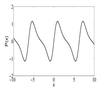
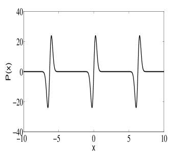
Figure 6: Potential $P(x)$. Left figure: $\alpha=1$; Right figure: $\alpha=16$.

For $\alpha=1$, the potential is smoother compared with $\alpha=16$, as it is shown in Figure 6. In Figure 6 we observe that $P(x)$ for $\alpha=1$ changes between $-1$ and $1$, whereas for $\alpha=16$ changes between $-20$ and $20$ and the change is not smooth. Our method can deal very well with both cases.

We consider the initial conditions,

$$n\left(x,0\right) = \frac{1}{L\sqrt{\pi}}e^{-x^{2}/L^{2}},{\ \ \ \ }\frac{\partial n}{\partial t}\left(x,0\right)=0,$$ (42)

$$j\left(x,0\right) = \frac{1}{L\sqrt{\pi}}e^{-x^{2}/L^{2}}\left(\frac{1}{L^{2}}2x+P(x)\right),$$ (43)

and the boundary conditions are given by

$$\lim_{x\rightarrow\infty}n(x,t)=0\quad\mbox{and}\quad\lim_{x\rightarrow-\infty}n(x,t)=0.$$

Note that the stationary solution of the problem is given by

$$n_{st}(x)=N_{r}\exp\left(-V(x)\right),$$

where $N_{r}$ is a normalization value.

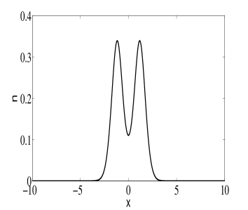
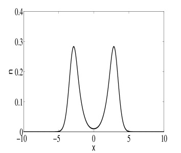
Figure 7: Particle density $n(x,t)$ for $\alpha=1$. Left figure: Curve for instant of time $t=1$; Right figure: Curve for instant of time $t=3$.

 

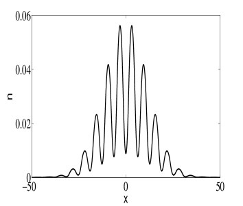
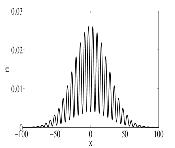
Figure 8: Particle density $n(x,t)$ for $\alpha=1$. Left figure: Curve for instant of time $t=100$ ;Right figure: Curve for instant of time $t=500$.

For $\alpha=1$ we show in Figures 7 and 8 the behaviour of the solution as we increase time from $t=1$ until $t=500$. The peak starts to split into two and then we have several waves forming that goes to the right and left. The domain where the function is not zero becomes larger as we travel in time. For that reason the computational domain increases considerably which requires more computational effort regarding the discretization in space. For an iterative method where we need to consider a discretization in time, it would require more computational effort for long times as we need to iterate in time whereas the Laplace transform has the advantage of not iterating in time and therefore it is the same if we compute the solution for short times or long times.

In Figure 9 we plot the flux for $\alpha=1$, as it evolves from $t=0$ to $t=1$ and in Figure 10 as it evolves from $t=5$ to $t=30$.

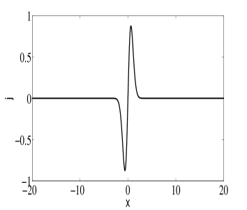
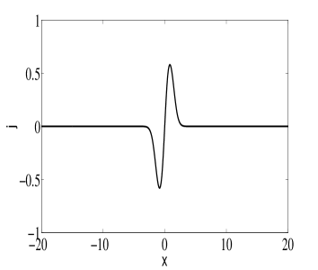
Figure 9: Density flux $j(x,t)$ for $\alpha=1$. Left figure: Curve for instant of time $t=0$; Right figure: Curve for instant of time $t=1$.

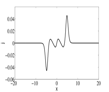
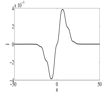
Figure 10: Density flux $j(x,t)$ for $\alpha=1$. Left figure: Curve for instant of time $t=5$; Right figure: Curve for instant of time $t=30$.

A quantity of physical interest in diffusion problems is the mean square displacement defined by

$$<x^{2}(t)>=\int_{-\infty}^{\infty}{[x^{2}n(x,t)]}dx.$$

For the Fickian case, $<x^{2}(t)>$ is linear in $t$ for all times in the absence of a potential. Now we would like to present calculations of $<x^{2}(t)>$ for the non-Fickian diffusion. At short times, and in the presence of a potential, the mean square displacement, $<x^{2}(t)>$, shows a $t^{2}$ behaviour, see Figure 11. This is due to inertial effects which are captured by a non-Fickian diffusion equation.

 

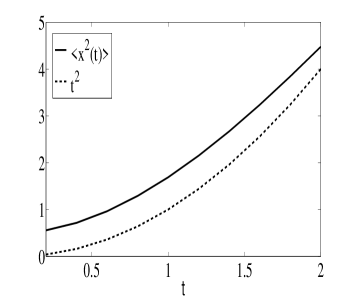
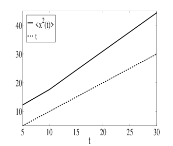
Figure 11: Mean square displacement for $\alpha=1$; Left figure: Curves for $t\in[0,2]$; Right figure: Curves for $t\in[5,30]$.

For $\alpha=16$ we show the evolution of the solution in the first instants of time. We see the solution presents very steep gradients and the method is able to give accurate solutions. First we observe how the wave split for $t=1$ and $t=2$ in Figure 12.

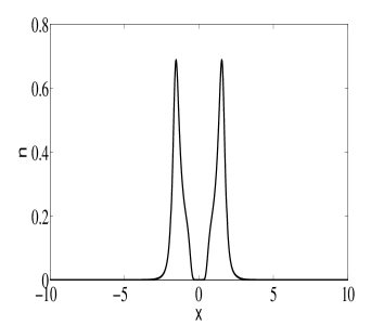
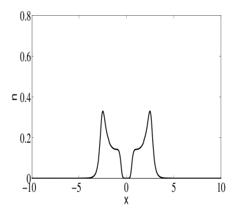
Figure 12: Particle density $n(x,t)$ for $\alpha=16$. Left figure: Curve for instant of time $t=1$; Right figure: Curve for instant of time $t=2$.

Next in Figure 13 we observe the behaviour for very large times. It is interesting to see how the Laplace method is able to give very quickly solutions for very large times. An iterative numerical method in time, it would take a large amount of time to run experiments for such long times such as $t=5000$ or $t=10000$ as we can see in Figure 14. The flux for $\alpha=16$ is plotted in Figure 15.

 

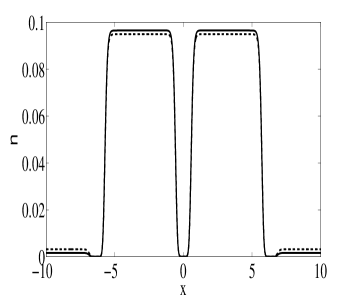
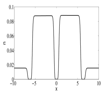
Figure 13: Particle density $n(x,t)$ for $\alpha=16$. Left figure: Curves for instant of times $t=500$ $(\--)$, $t=1000$ $(\--\--)$; Right figure: Curve for instant of time $t=5000$ $(\--)$.

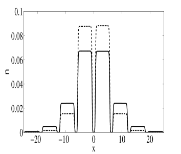
Figure 14: Particle density $n(x,t)$ for $\alpha=16$. Curves for instant of time $t=5000$ $(\--\--)$; $t=10000$ $(\--)$.

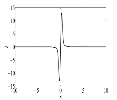
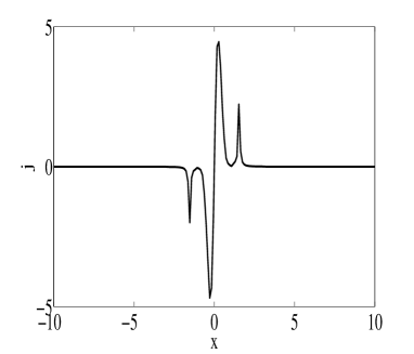
Figure 15: Density flux for $\alpha=16$. Left figure: Curve for instant of time $t=0$; Right figure: Curve for instant of time $t=1$.

6 Summary and outlook

In this paper we have presented a numerical solution of a non-Fickian diffusion equation which is a partial differential equation of the hyperbolic type. This equation is of physical interest in the context of Brownian motion in inertial as well as diffusive regimes. In our model the Brownian particle is subjected to a symmetric periodic potential of flexible shapes (generated with a single variable parameter) which can lead to harmonic, anharmonic or a confining potential for the particle.

Instead of introducing discretization in both space and time variables we dealt with the time-derivatives through time Laplace transform and obtained an ordinary differential equation in space variable. This equation was then solved with a finite-difference scheme, leading to a discretised approximate solution for $\widetilde{n}(x,s)$; the solution is approximate due to discretization and is still formally exact in the Laplace domain $s$. The next step consisted of numerical Laplace inversion to obtain an approximation to the original solution $n(x,t)$. We show that the full method is second order accurate; this finding receives additional support from two test examples considered in Section 4. One may be able to consider further improvement. A major advantage of using the time Laplace transform is that we can compute the approximate solution for long times accurately and quickly. Any iterative numerical method would take too long to compute the solution for similar times even if we consider an unconditionally implicit numerical method which will allow large time steps. Additionally, our algorithm takes into consideration the smoothness of the solution; in other words the computational effort is higher in the regions where the solution has steep gradients. Another merit of the method is that it can be easily generalized to higher spatial dimensions. It would be of interest to consider an application of the method to numerically solve the Kramers equation which is a more involved partial differential equation than the non-Fickian diffusion equation.

References

- [1] J. Abate, W. Whitt, Numerical inversion of Laplace transforms of probability distributions, ORSA Journal on Computing, 7(1): 36–43, 1995.
- [2] J. Ahn, S. Kang, Y. Kwon, A flexible inverse Laplace transform algorithm and its application, Computing 71(2): 115–131, 2003.
- [3] G. Bao, G.W. Wei, S. Zhao, Numerical solution of the Helmholtz equation with high wavenumbers, International Journal for Numerical Methods in Engineering 59: 389–408, 2004.
- [4] G. Barbero, J. R. Macdonald, Transport process of ions in insulating media in the hyperbolic diffusion regime, Phys. Rev. E 81: 051503, 2010.
- [5] A.C. Branka, A.K. Das, D.M. Heyes, Overdamped Brownian motion in periodic symmetric potentials, J.Chem.Phys. 113: 9911, 2000.
- [6] K. Crump, Numerical inversion of Laplace transforms using a Fourier series approximation, Journal of the Association for Computing Machinery 23(1): 89–96, 1976.
- [7] J. Crank, P. Nicolson, A practical method for numerical evaluation of solutions of partial differential equations of the heat conduction type, Proc. Cambridge Phil. Soc. 43: 50–67, 1947.
- [8] A.K. Das, A non-fickian diffusion equation, J.Appl.Phys. 70(3): 1355–1358, 1991.
- [9] G. Fibich, B. Ilan, S. Tsynkov, Backscattering and nonparaxiality arrest collapse of damped nonlinear waves, SIAM J. Appl. Math. 63(5): 1718–1736, 2003.
- [10] J. Fort, V. Méndez, Wavefronts in time-delayed reaction-diffusion systems. Theory and comparison to experiment, Rep. Prog. Phys. 65: 895–954, 2002.
- [11] R. Huang et al, Direct observation of the full transition from ballistic to diffusive Brownian motion in a liquid, Nature Physics, NPHYS1953, 2011.
- [12] T. Li, S. Kheifets, D. Medellin, M. G. Raizen, Measurement of the instantaneous velocity of a brownian particle, Science 25(328): 1673–1675, 2010.
- [13] M.O. Magnasco, Forced thermal ratchets, Physical Review Letters 71: 1477–1481, 1993.
- [14] J.E. Marsden, M.J. Hoffman, Basic Complex Analysis, W.H. Freeman, 1999.
- [15] C. Neves, A. Araújo, E. Sousa, Numerical approximation of a transport equation with a time-dependent dispersion flux, in AIP Conference Proceedings 1048: 403–406, 2008.
- [16] F.S.B.F. Oliveira, K. Anastasiou, An efficient computational model for water wave propagation in coastal regions, Applied Ocean Research, 20(5): 263–271, 1998.
- [17] P.N. Pusey, Brownian motion goes ballistic, Science 332: 802–803, 2011.
- [18] K. Wang, C. You, A note on identifying generalized diagonally dominant matrices, International Journal of Computer Mathematics 84(12): 1863-1870, 2007.
- [19] R.S. Varga, Matrix Iterative Analysis, Springer, 2000.