A weighted finite difference method for the fractional diffusion equation based on the Riemann-Liouville derivative

Abstract

A one dimensional fractional diffusion model with the Riemann-Liouville fractional derivative is studied. First, a second order discretization for this derivative is presented and then an unconditionally stable weighted average finite difference method is derived. The stability of this scheme is established by von Neumann analysis. Some numerical results are shown, which demonstrate the efficiency and convergence of the method. Additionally, some physical properties of this fractional diffusion system are simulated, which further confirm the effectiveness of our method.

1 Introduction

Recently, a large number of applied problems have been formulated on fractional differential equations and consequently considerable attention has been given to the solutions of those equations. Fractional space derivatives are used to model anomalous diffusion or dispersion, a phenomenon observed in many problems. There are some diffusion processes for which the Fick’s second law fails to describe the related transport behavior. This phenomenon is called anomalous diffusion, which is characterized by the nonlinear growth of the mean square displacement, of a diffusion particle over time. The anomalous diffusions differ according to the values of $\alpha$, where $\alpha$ is the order of the fractional derivative. Some works providing an introduction to fractional calculus related to diffusion problems are, for instance, [2, 6, 11, 12, 28, 29]. In this work we will be interested in the anomalous diffusion, called supperdiffusion, for $1<\alpha<2$ and experimental evidence of this type of diffusion is already reported in several works [1, 7, 13, 14].

Fractional derivatives are non-local opposed to the local behaviour of integer derivatives. Therefore, different challenges appear when we try to derive numerical methods for this type of equations. Numerical approaches to different types of fractional diffusion models are increasingly appearing in literature. We can found recent work on numerical solutions for the fractional diffusion equation describing superdiffusion [5, 9, 10, 19, 15, 27, 16] and also for several transport equations including this type of diffusion [18, 25, 31]. Some other works consider subdiffusion, which is represented by a time fractional derivative of positive order and less than one [3, 30]. However, the challenges for these equations are different from the ones that arise when we consider a space fractional derivative of order $1\leq\alpha<2$.

Numerical methods, for models with superdiffusion, have been obtained with mathematical techniques which do not necessarily consider a second order discretization for the fractional derivative to achieve second order accuracy. In this work, we present a second order approximation for the fractional Riemann-Liouville derivative of order $\alpha$, $1<\alpha<2$. This approach uses some of the tools described in [4, 8] and also applied in [26] to derive an approximation for the Caputo fractional derivative defined in bounded domains. Here, we consider the Riemann-Liouville fractional derivative in an unbounded domain and its discretization is represented by a series instead of a finite sum. We prove the order of consistency of this discretization is second order.

A weighted average finite difference $\tau$-scheme is considered, for $\tau\in[1/2,1]$, which includes the Crank-Nicolson method ($\tau=1/2$) and the back forward Euler method ($\tau=1$). The consistency and stability of the $\tau$-scheme are established and we prove the $\tau$-scheme is unconditionally stable. Also for $\tau=1/2$ we have second order accuracy in time and space as expected.

Consider the one-dimensional fractional diffusion equation [1, 7, 16]

$$\frac{\partial u}{\partial t}(x,t)=d(x)\frac{\partial^{\alpha}u}{\partial x^{\alpha}}(x,t)+p(x,t)$$ (1)

on the domain $x\in{\rm I\kern-1.69998ptR}$, where $1<\alpha\leq 2$ and $d(x)>0$, subject to the initial condition

$$u(x,0)=f(x),\ x\in{\rm I\kern-1.69998ptR}$$ (2)

and to the boundary condition

$$u(x,t)=0\quad\mbox{as}\quad|x|\rightarrow\infty.$$ (3)

The usual way of representing the fractional derivatives is by the Riemann-Liouville formula. The Riemann-Liouville fractional derivative of order $\alpha$, for $x\in[a,b]$, $-\infty\leq a<b\leq\infty$, is defined by

$$\frac{\partial^{\alpha}u}{\partial x^{\alpha}}(x,t)=\frac{1}{\Gamma(n-\alpha)}\frac{\partial^{n}}{\partial x^{n}}\int_{a}^{x}{u(\xi,t)}{(x-\xi)^{n-\alpha-1}}d\xi,\quad(n-1<\alpha<n)$$ (4)

where $\Gamma(\cdot)$ is the Gamma function and $n=[\alpha]+1$, with $[\alpha]$ denoting the integer part of $\alpha$.

The function $u(x,t)$ under consideration, that is, which is solution of (1), should be such that the corresponding integral (4) converges. If the function $u(x,t)$ vanishes at infinity, as assumed when we impose the boundary condition (3), we have absolute convergence of such integrals for a wide class of functions [24]. However, these functions do not necessarily need to vanish at infinity and we can found under which conditions these integrals converge in [24] (section 14.3). There are very complete works about the fractional calculus [17, 20, 21, 22, 24], where the theoretical properties of this type of derivative are studied in detail.

Another way to represent the fractional derivative is by the Grünwald-Letnikov formula, that is,

$$\frac{\partial^{\alpha}u}{\partial x^{\alpha}}(x,t)=\lim_{\Delta x\rightarrow 0}\frac{1}{\Delta x^{\alpha}}\sum_{k=0}^{\left[\frac{x-a}{\Delta x}\right]}(-1)^{k}\left(\begin{array}[]{c}\alpha\\ k\end{array}\right)u(x-k\Delta x,t).\quad(\alpha>0)$$ (5)

The Grünwald-Letnikov approximation is often used to numerically approximate the Riemann-Liouville derivative and it was the first algorithm to appear for approximating fractional derivatives [21, 22]. However, this approximation has consistency of order one and also very frequently numerical approximations based in this formula originate unstable numerical methods and henceforth a shifted Grünwald-Letnikov formula is used [16, 18].

The plan of the paper is as follows. In section 2 we derive a numerical approximation for the Riemann-Liouville derivative. The full discretisation of the fractional diffusion equation is given in section 3, where a weighted finite difference method in time is applied with the weight $\tau\in[1/2,1]$. In section 4 we prove the convergence of the numerical method by showing consistency and stability. In the fifth section we present numerical results which confirm the theoretical results and in the last section we give some conclusions.

2 The numerical method

In this section we present a numerical approximation for the Riemann-Liouville derivative and also the numerical method that gives an approximate solution to the fractional diffusion equation.

2.1 Approximation of the Riemann-Liouville derivative

Let us consider the Riemann-Liouville derivative [21, 22], that is,

$$\frac{\partial^{\alpha}u}{\partial x^{\alpha}}(x,t)=\frac{1}{\Gamma(2-\alpha)}\frac{\partial^{2}}{\partial x^{2}}\int_{-\infty}^{x}{u(\xi,t)}{(x-\xi)^{1-\alpha}}d\xi,\quad 1<\alpha<2.$$ (6)

We define the mesh points $x_{j}=j\Delta x,\ j\in\mathbb{Z}$ where $\Delta x$ denotes the uniform space step. For a fixed time $t$, let us denote

$${\cal I}_{\alpha}(x)=\int_{-\infty}^{x}{u(\xi,t)}{(x-\xi)^{1-\alpha}}d\xi.$$ (7)

First, we do the following approximation at $x_{j}$

$$\frac{\partial^{2}}{\partial x^{2}}{\cal I}_{\alpha}(x_{j})\simeq\frac{1}{\Delta x^{2}}\left[{\cal I}_{\alpha}(x_{j-1})-2{\cal I}_{\alpha}(x_{j})+{\cal I}_{\alpha}(x_{j+1})\right].$$

For each $x_{j}$ we need to calculate ${\cal I}_{\alpha}(x_{j})$.

We compute these integrals by approximating $u(\xi,t)$, at a fixed instant $t$, by a linear spline $s_{j}(\xi)$, whose nodes and knots are chosen at $x_{k}$, $k=\dots,j-1,j$, that is, an approximation to ${\cal I}_{\alpha}(x_{j})$ becomes $I_{\alpha}(x_{j})$ defined by

$$I_{\alpha}(x_{j})=\int_{-\infty}^{x_{j}}{s_{j}}(\xi){(x_{j}-\xi)^{1-\alpha}}d\xi.$$ (8)

The spline $s_{j}(\xi)$ interpolates the points $\{(x_{k},t):\ k\leq j\}$ and is of the form [23]

$$s_{j}(\xi)=\sum_{k=-\infty}^{j}u(x_{k},t)s_{j,k}(\xi),$$ (9)

with $s_{j,k}(\xi)$, in each interval $[x_{k-1},x_{k+1}]$, for $k\leq j-1$, given by

$$s_{j,k}(\xi)=\left\{\begin{array}[]{cc}\displaystyle{\frac{\xi-x_{k-1}}{x_{k}-x_{k-1}}},&x_{k-1}\leq\xi\leq x_{k}\\ &\\ \displaystyle{\frac{x_{k+1}-\xi}{x_{k+1}-x_{k}}},&x_{k}\leq\xi\leq x_{k+1}\\ &\\ 0&\mbox{otherwise,}\end{array}\right.$$ (10)

and for $k=j$,

$$s_{j,j}(\xi)=\left\{\begin{array}[]{cc}\displaystyle{\frac{\xi-x_{j-1}}{x_{j}-x_{j-1}}},&x_{j-1}\leq\xi\leq x_{j}\\ &\\ 0&\mbox{otherwise.}\end{array}\right.$$ (11)

From (8) and (9),

$$I_{\alpha}(x_{j})=\sum_{k=-\infty}^{j}u(x_{k},t)\int_{x_{k-1}}^{x_{k+1}}s_{j,k}(\xi)(x_{j}-\xi)^{1-\alpha}d\xi.$$ (12)

We have that

$$\int_{x_{k-1}}^{x_{k+1}}s_{j,k}(\xi)(x_{j}-\xi)^{1-\alpha}d\xi = \int_{x_{k-1}}^{x_{k}}\frac{\xi-x_{k-1}}{\Delta x}(x_{j}-\xi)^{1-\alpha}+\int_{x_{k}}^{x_{k+1}}\frac{x_{k+1}-\xi}{\Delta x}(x_{j}-\xi)^{1-\alpha}{}$$ (13)

$$= \frac{\Delta x^{2-\alpha}}{(2-\alpha)(3-\alpha)}a_{j,k},$$

where the $a_{j,k}$ are such that,

$$a_{j,k}=\left\{\begin{array}[]{cc}(j-k+1)^{3-\alpha}-2(j-k)^{3-\alpha}+(j-k-1)^{3-\alpha},&\ k\leq j-1\\ &\\ 1,&\ k=j.\end{array}\right.$$ (14)

Therefore,

$$I_{\alpha}(x_{j})=\frac{\Delta x^{2-\alpha}}{(2-\alpha)(3-\alpha)}\sum_{k=-\infty}^{j}u(x_{k},t)a_{j,k},$$ (15)

and an approximation for $\displaystyle{\frac{\partial^{2}}{\partial x^{2}}{\cal I}_{\alpha}(x_{j})}$, is given by,

$$\frac{1}{\Delta x^{2}}\left[I_{\alpha}(x_{j-1})-2I_{\alpha}(x_{j})+I_{\alpha}(x_{j+1})\right]$$ (16)

that is,

$$\frac{\Delta x^{-\alpha}}{(2-\alpha)(3-\alpha)}\left[\sum_{k=-\infty}^{j-1}u(x_{k},t)a_{j-1,k}-2\sum_{k=-\infty}^{j}u(x_{k},t)a_{j,k}+\sum_{k=-\infty}^{j+1}u(x_{k},t)a_{j+1,k}\right].$$

Let us assume there are approximations ${\bf U}^{n}:=\{U_{j}^{n}\}$ to the values $u(x_{j},t_{n})$, where $t_{n}=n\Delta t,\ n\geq 0$ and $\Delta t$ is the uniform time-step.

We define the fractional operator as

$$\delta_{\alpha}U_{j}^{n}=\frac{1}{\Gamma(4-\alpha)}\left\{\sum_{k=-\infty}^{j+1}q_{j,k}U_{k}^{n}\right\},$$ (17)

where

$$q_{j,k} = a_{j-1,k}-2a_{j,k}+a_{j+1,k},\quad k\leq j-1{}$$

$$q_{j,j} = -2a_{j,j}+a_{j+1,j}{}$$

$$q_{j,j+1} = a_{j+1,j+1}.$$ (18)

Therefore, an approximation of (6), for $t=t_{n}$, can be given by $\displaystyle{\frac{\delta_{\alpha}U_{j}^{n}}{\Delta x^{\alpha}}}.$

We can also write the fractional operator (17) as

$$\delta_{\alpha}U_{j}^{n}=\frac{1}{\Gamma(4-\alpha)}\sum_{m=-1}^{\infty}q_{j,j-m}U_{j-m}^{n}.$$ (19)

Remark: Note that for $\alpha=1$ and $\alpha=2$ the coefficients (18) are such that $q_{j,k}=0$, for $k<j-1$. For $\alpha=1$, $q_{j,j-1}=-1$, $q_{j,j}=0$, $q_{j,j+1}=1$ and for $\alpha=2$, $q_{j,j-1}=1$, $q_{j,j}=-2$, $q_{j,j+1}=1$.

Remark: The series (19) converges absolutely for each $1<\alpha<2$ and for every bounded function $u(x,t)$, for a fixed $t$. This result is a straightforward consequence of some results given in section 3 about the convergence of the series of the $q_{j,j-m}$.

In this section we have considered a linear spline to approximate the integral representation of the Riemann-Liouville derivative with the purpose of obtaining a second order approximation. In the next section we describe the full discretisation of the differential equation.

2.2 Weighted average finite difference methods

We discretize the spatial $\alpha$-order derivative following the steps of the previous section. The discretization in time consists of the weighted average discretization.

We consider the time discretization $0\leq t_{n}\leq T$. Additionally, let $d_{j}=d(x_{j})$, $p_{j}^{n}=p(x_{j},t_{n})$. For the uniform space step $\Delta x$ and time step $\Delta t$, let

$$\mu_{j}^{\alpha}=\frac{d_{j}\Delta t}{{\Delta x}^{\alpha}}.$$

From equation (1) we can arrive at the explicit Euler and implicit Euler numerical methods, respectively

$$\frac{U_{j}^{n+1}-U_{j}^{n}}{\Delta t}=\frac{d_{j}}{\Delta x^{\alpha}}\delta_{\alpha}U^{n}_{j}+p^{n}_{j},~{}~{}~{}$$ (20)

$$\frac{U_{j}^{n+1}-U_{j}^{n}}{\Delta t}=\frac{d_{j}}{\Delta x^{\alpha}}\delta_{\alpha}U^{n+1}_{j}+p^{n+1}_{j},~{}~{}~{}$$ (21)

Let (20) multiplies $(1-\tau)$ and (21) multiplies $\tau$. We obtain the following weighted $\tau$-scheme

$${U_{j}^{n+1}-U_{j}^{n}}=\mu_{j}^{\alpha}\bigg{\{}(1-\tau)\delta_{\alpha}U^{n}_{j}+\tau\delta_{\alpha}U^{n+1}_{j}\bigg{\}}+\tau\Delta tp^{n+1}_{j}+(1-\tau)\Delta tp^{n}_{j},$$ (22)

where $\tau\in[1/2,1]$.

Note that for $\alpha=2$, the operator (17) is the central second order operator $\delta^{2}U_{j}^{n}$, that is,

$$\delta_{\alpha}U_{j}^{n}=U_{j+1}^{n}-2U_{j}^{n}+U_{j-1}^{n}.$$

We have the following numerical method

$$\left(1-\tau{\mu_{j}^{\alpha}}\delta_{\alpha}\right)U_{j}^{n+1}=\left(1+(1-\tau){\mu_{j}^{\alpha}}\delta_{\alpha}\right)U_{j}^{n}+\Delta tp_{j}^{n+\tau},$$ (23)

where

$$p_{j}^{n+\tau}=\tau p_{j}^{n}+(1-\tau)p_{j}^{n+1}.$$

3 Convergence of the numerical scheme

In this section we prove the convergence of the numerical method by showing it is consistent and von Neumann stable. First, we start to study the consistency of the numerical method and lastly we present the stability results.

3.1 Consistency

In the beginning of this section, for the sake of clarity, we omit the variable $t$ and we denote the partial derivative of $u$ in $x$ of order $r$ by $u^{(r)}$.

Lemma 1

Let $u\in C^{(4)}({\rm I\kern-1.69998ptR})$. For $\xi\in[x_{k-1},x_{k}]$,

$$u(\xi)-s_{j,k}(\xi)=-\frac{1}{r!}\sum_{r=2}^{3}u^{(r)}(\xi)l_{k,r}(\xi)-\frac{1}{4!}u^{(4)}(\eta_{k})l_{k,r}(\xi),\ \eta_{k}\in[x_{k-1},x_{k}],$$

where

$$|l_{k,r}(\xi)|\leq\Delta x^{r}.$$

Proof: For $\xi\in[x_{k-1},x_{k}]$,

$$u(\xi)-s_{j,k}(\xi)=u(\xi)-\frac{x_{k}-\xi}{\Delta x}u(x_{k-1})-\frac{\xi-x_{k-1}}{\Delta x}u(x_{k}).$$

Using Taylor expansions, we obtain

$$u(\xi)-s_{j,k}(\xi) = -\frac{1}{r!}\sum_{r=2}^{3}u^{(r)}(\xi)l_{k,r}(\xi)-\frac{1}{4!}u^{(4)}(\eta_{k})l_{k,r}(\xi),$$

where $l_{k,r}(\xi)$ are functions which depend on $\Delta x$ and $x_{k}$, given by

$$l_{k,r}(\xi) = \frac{x_{k}-\xi}{\Delta x}(x_{k}-\xi-\Delta x)^{r}-\frac{\xi-x_{k}+\Delta x}{\Delta x}(x_{k}-\xi)^{r}$$ (24)

$$= (x_{k}-\xi)^{r}+\sum_{r=0}^{p-1}\left(\begin{array}[]{c}r\\ p\end{array}\right)(x_{k}-\xi)^{p+1}(-1)^{r-p}\Delta x^{r-p-1}.$$ (27)

It is easy to conclude that $|l_{k,r}(\xi)|\leq\Delta x^{r}$, for $\xi\in[x_{k-1},x_{k}]$. $\square$

Theorem 2

(Order of accuracy of the approximation for the fractional derivative): Let $u\in C^{(4)}({\rm I\kern-1.69998ptR})$ and such that $u^{(4)}(x)=0$, for $x\leq a$, being $a$ a real constant. We have that

$$\frac{\partial^{\alpha}u}{\partial x^{\alpha}}(x_{j})-\frac{\delta_{\alpha}u}{\Delta x^{\alpha}}(x_{j})=\epsilon_{1}(x_{j})+\epsilon_{2}(x_{j}),$$

where

$$|\epsilon_{1}(x_{j})|\leq C_{1}\Delta x^{2}\quad\quad|\epsilon_{2}(x_{j})|\leq C_{2}\Delta x^{2},$$

and $C_{1}$ and $C_{2}$ are independent of $\Delta x$.

Proof: It is straightforward to prove that we have

$$\frac{\partial^{\alpha}u}{\partial x^{\alpha}}(x_{j}) = \frac{1}{\Gamma(2-\alpha)}\frac{\partial^{2}}{\partial x^{2}}{\cal I}_{\alpha}(x_{j})$$

$$= \frac{1}{\Gamma(2-\alpha)}\frac{1}{\Delta x^{2}}\left[{\cal I}_{\alpha}(x_{j-1})-2{\cal I}_{\alpha}(x_{j})+{\cal I}_{\alpha}(x_{j+1})\right]+\epsilon_{1}(x_{j}),$$

where $\epsilon_{1}(x_{j})={\cal O}(\Delta x^{2})$.

Let us define the error $E_{S}(x_{j})$, such that,

$${\cal I}_{\alpha}(x_{j-1})-2{\cal I}_{\alpha}(x_{j})+{\cal I}_{\alpha}(x_{j+1})={I}_{\alpha}(x_{j-1})-2{I}_{\alpha}(x_{j})+{I}_{\alpha}(x_{j+1})+E_{S}(x_{j}).$$

We have

$$\frac{\partial^{\alpha}u}{\partial x^{\alpha}}(x_{j}) = \frac{1}{\Gamma(2-\alpha)}\frac{1}{\Delta x^{2}}\left[{\cal I}_{\alpha}(x_{j-1})-2{\cal I}_{\alpha}(x_{j})+{\cal I}_{\alpha}(x_{j+1})\right]$$

$$+\frac{1}{\Gamma(2-\alpha)}\frac{1}{\Delta x^{2}}E_{S}(x_{j})+\epsilon_{1}(x_{j}),$$

that is

$$\frac{\partial^{\alpha}u}{\partial x^{\alpha}}(x_{j})=\frac{\delta_{\alpha}u}{\Delta x^{\alpha}}(x_{j})+\epsilon_{1}(x_{j})+\epsilon_{2}(x_{j}),$$

where

$$\epsilon_{2}(x_{j})=\frac{1}{\Gamma(2-\alpha)}\frac{1}{\Delta x^{2}}E_{S}(x_{j}).$$

We are now going to compute the error $E_{S}(x_{j})$. We have

$$E_{S}(x_{j}) = \sum_{k=-\infty}^{j-1}\ \int_{x_{k-1}}^{x_{k}}(u(\xi)-s_{j-1,k}(\xi))(x_{j-1}-\xi)^{1-\alpha}d\xi$$

$$-2\sum_{k=-\infty}^{j}\ \int_{x_{k-1}}^{x_{k}}(u(\xi)-s_{j,k}(\xi))(x_{j}-\xi)^{1-\alpha}d\xi$$

$$+\sum_{k=-\infty}^{j+1}\ \int_{x_{k-1}}^{x_{k}}(u(\xi)-s_{j+1,k}(\xi))(x_{j+1}-\xi)^{1-\alpha}d\xi.$$

Taking in consideration the previous lemma, let us denote

$$E_{S}(x_{j})=-\sum_{r=2}^{4}\frac{1}{r!}E_{r}(x_{j}),$$ (28)

where $E_{r}(x_{j})$ are defined as follows. For $r=2$ and $r=3$,

$$E_{r}(x_{j}) = \sum_{k=-\infty}^{j-1}\ \int_{x_{k-1}}^{x_{k}}l_{{k},r}(\xi)u^{(r)}(\xi)(x_{j-1}-\xi)^{1-\alpha}d\xi$$ (29)

$$-2\sum_{k=-\infty}^{j}\ \int_{x_{k-1}}^{x_{k}}l_{{k},r}(\xi)u^{(r)}(\xi)(x_{j}-\xi)^{1-\alpha}d\xi$$

$$+\sum_{k=-\infty}^{j+1}\ \int_{x_{k-1}}^{x_{k}}l_{{k},r}(\xi)u^{(r)}(\xi)(x_{j+1}-\xi)^{1-\alpha}d\xi,$$

and for $r=4$

$$E_{r}(x_{j}) = \sum_{k=-\infty}^{j-1}\ u^{(4)}(\eta_{k})\int_{x_{k-1}}^{x_{k}}l_{{k},r}(\xi)(x_{j-1}-\xi)^{1-\alpha}d\xi$$ (30)

$$-2\sum_{k=-\infty}^{j}u^{(4)}(\eta_{k})\ \int_{x_{k-1}}^{x_{k}}l_{{k},r}(\xi)(x_{j}-\xi)^{1-\alpha}d\xi$$

$$+\sum_{k=-\infty}^{j+1}u^{(4)}(\eta_{k})\ \int_{x_{k-1}}^{x_{k}}l_{{k},r}(\xi)(x_{j+1}-\xi)^{1-\alpha}d\xi.$$

For $r=2,3$ by changing variables, we obtain

$$E_{r}(x_{j}) = \sum_{k=-\infty}^{j}\ \int_{x_{k-1}}^{x_{k}}l_{k,r}(\xi)u^{(r)}(\xi-\Delta x)(x_{j}-\xi)^{1-\alpha}d\xi$$

$$-2\sum_{k=-\infty}^{j}\ \int_{x_{k-1}}^{x_{k}}l_{k,r}(\xi)u^{(r)}(\xi)(x_{j}-\xi)^{1-\alpha}d\xi$$

$$+\sum_{k=-\infty}^{j}\ \int_{x_{k-1}}^{x_{k}}l_{k,r}(\xi)u^{(r)}(\xi+\Delta x)(x_{j}-\xi)^{1-\alpha}d\xi,$$

that is,

$$E_{r}(x_{j}) = \sum_{k=-\infty}^{j}\ \int_{x_{k-1}}^{x_{k}}l_{k,r}(\xi)\left[u^{(r)}(\xi+\Delta x)-2u^{(r)}(\xi)+u^{(r)}(\xi-\Delta x)\right](x_{j}-\xi)^{1-\alpha}d\xi.$$

Let $x_{a}=N_{a}\Delta x$ such that $u^{(4)}(x)=0$, for $x\leq x_{a}$. For $r=2$ we have

$$E_{2}(x_{j}) = \sum_{k=-\infty}^{j}\ \int_{x_{k-1}}^{x_{k}}l_{k,2}(\xi)\left[u^{(r)}(\xi+\Delta x)-2u^{(r)}(\xi)+u^{(r)}(\xi-\Delta x)\right](x_{j}-\xi)^{1-\alpha}d\xi$$

$$= \frac{\Delta x^{2}}{2}\sum_{k=N_{a}+1}^{j}u^{(4)}(\xi_{k})c_{j,k,2},\quad\xi_{k}\in[x_{k-1},x_{k}]$$

where

$$c_{j,k,2}=\int_{x_{k-1}}^{x_{k}}l_{k,r}(\xi)(x_{j}-\xi)^{1-\alpha}d\xi$$

Since, by Lemma 1,

$$|c_{j,k,2}|\leq\Delta x^{2}\int_{x_{k-1}}^{x_{k}}(x_{j}-\xi)^{1-\alpha}d\xi$$

and

$$\int_{x_{a}}^{x_{j}}(x_{j}-\xi)^{1-\alpha}d\xi=\frac{1}{2-\alpha}{(x_{j}-x_{a})^{2-\alpha}}$$

we have

$$|E_{2}(x_{j})|\leq\frac{\Delta x^{4}}{2(2-\alpha)}||u^{(4)}||_{\infty}(x_{j}-x_{a})^{2-\alpha}.$$ (31)

For $r=3$,

$$E_{3}(x_{j})=\sum_{k=N_{a}+1}^{j}\Delta x(u^{(4)}(\xi_{k_{1}})-u^{(4)}(\xi_{k_{2}}))c_{j,k,3},\ \xi_{k_{1}},\xi_{k_{2}}\in[x_{k-1},x_{k}]$$

and

$$|c_{j,k,3}|\leq\Delta x^{3}\int_{x_{k-1}}^{x_{k}}(x_{j}-\xi)^{1-\alpha}d\xi.$$

We have

$$|E_{3}(x_{j})|\leq\frac{2\Delta x^{4}}{(2-\alpha)}||u^{(4)}||_{\infty}(x_{j}-x_{a})^{2-\alpha}.$$ (32)

Finally for $r=4$, we bound each integral of (30) separately. For the first integral we have

$$\sum_{k=N_{a}+1}^{j-1}u^{(4)}(\eta_{k})\int_{x_{k-1}}^{x_{k}}l_{k,4}(\xi)(x_{j-1}-\xi)^{1-\alpha}d\xi$$

$$\leq \Delta x^{4}||u^{(4)}||_{\infty}\sum_{k=N_{a}+1}^{j-1}\int_{x_{k-1}}^{x_{k}}(x_{j-1}-\xi)^{1-\alpha}d\xi$$

$$= \frac{\Delta x^{4}}{2-\alpha}||u^{(4)}||_{\infty}(x_{j-1}-x_{a})^{2-\alpha}.$$

Therefore, since $(a+b)^{p}\leq|a|^{p}+|b|^{p}$ for $0<p\leq 1$, we have

$$\sum_{k=N_{a}+1}^{j-1}u^{(4)}(\eta_{k})\int_{x_{k-1}}^{x_{k}}l_{k,4}(\xi)(x_{j-1}-\xi)^{1-\alpha}d\xi\leq\frac{\Delta x^{4}}{2-\alpha}||u^{(4)}||_{\infty}((x_{j}-x_{a})^{2-\alpha}+\Delta x^{2-\alpha}).$$

Similarly, for the second integral we have

$$\sum_{k=N_{a}+1}^{j}u^{(4)}(\eta_{k})\int_{x_{k-1}}^{x_{k}}l_{k,4}(\xi)(x_{j}-\xi)^{1-\alpha}d\xi\leq\frac{\Delta x^{4}}{2-\alpha}||u^{(4)}||_{\infty}(x_{j}-x_{a})^{2-\alpha}$$

and for the third integral

$$\sum_{k=N_{a}+1}^{j+1}u^{(4)}(\eta_{k})\int_{x_{k-1}}^{x_{k}}l_{k,4}(\xi)(x_{j+1}-\xi)^{1-\alpha}d\xi\leq\frac{\Delta x^{4}}{2-\alpha}||u^{(4)}||_{\infty}((x_{j}-x_{a})^{2-\alpha}+\Delta x^{2-\alpha}).$$

Finally, we have

$$|E_{4}(x_{j})|\leq\frac{3\Delta x^{4}}{2-\alpha}||u^{(4)}||_{\infty}(x_{j}-x_{a})^{2-\alpha}+\frac{2\Delta x^{6-\alpha}}{2-\alpha}||u^{(4)}||_{\infty}.$$ (33)

From (31), (32) and (33) it is easy to conclude that the error $E_{S}(x_{j})$ defined by (83) is of order $\mathcal{O}(\Delta x^{4})$ and therefore the $\epsilon_{2}(x_{j})$ is of order $\mathcal{O}(\Delta x^{2})$.

$\square$

Theorem 3

The truncation error of the weighted numerical method (23) is of order ${\cal O}(\Delta x^{2})+{\cal O}(\Delta t^{m_{\tau}})$, where $m_{\tau}=1$, for $\tau\in(1/2,1]$ and $m_{\tau}=2$, for $\tau=1/2$.

Proof: Let $u=u(x,t)$ be a solution to the fractional partial differential equation and satisfying the conditions of the previous theorem. Note that the truncation error for the numerical method (23) is given by

$$T_{j}^{n}=\frac{u_{j}^{n+1}-u_{j}^{n}}{\Delta t}-\frac{d_{j}}{\Delta x^{\alpha}}\left(\tau\delta_{\alpha}u_{j}^{n+1}+(1-\tau)\delta_{\alpha}u_{j}^{n}\right)-p_{j}^{n+\tau}.$$

We have that

$$\frac{u_{j}^{n+1}-u_{j}^{n}}{\Delta t}=\frac{\partial u(x_{j},t_{n})}{\partial t}+\frac{\Delta t}{2}\frac{\partial^{2}u(x_{j},t_{n})}{\partial t^{2}}+O(\Delta t^{2}),$$ (34)

and using the previous theorem we have

$$T_{j}^{n} = \frac{\partial u(x_{j},t_{n})}{\partial t}+\frac{\Delta t}{2}\frac{\partial^{2}u(x_{j},t_{n})}{\partial t^{2}}+O(\Delta t^{2})-\tau\bigg{(}d_{j}\frac{\partial^{\alpha}u(x_{j},t_{n+1})}{\partial x^{\alpha}}+O(\Delta x^{2})\bigg{)}$$

$$-(1-\tau)\bigg{(}d_{j}\frac{\partial^{\alpha}u(x_{j},t_{n})}{\partial x^{\alpha}}+O(\Delta x^{2})\bigg{)}-p^{n+\tau}_{j}.$$

Therefore

$$T_{j}^{n} = \frac{\partial u(x_{j},t_{n})}{\partial t}+\frac{\Delta t}{2}\frac{\partial^{2}u(x_{j},t_{n})}{\partial t^{2}}+-(1-\tau)\frac{\partial u(x_{j},t_{n})}{\partial t}-\tau\frac{\partial u(x_{j},t_{n+1})}{\partial t}$$

$$+O(\Delta t^{2})+O(\Delta x^{2})$$

Finally,

$$T_{j}^{n} = (\frac{1}{2}-\tau)\Delta t\frac{\partial^{2}u(x_{j},t_{n})}{\partial t^{2}}+O(\Delta t^{2})+O(\Delta x^{2}).$$

$\square$

3.2 Fourier decomposition of the error

In order to derive stability conditions for the finite difference schemes, we apply the von Neumann analysis or Fourier analysis. Fourier analysis assumes that we have a solution defined in the whole real line. It is also applied to problems defined in finite domains with periodic boundary conditions since the solution is seen as a periodic function in ${\rm I\kern-1.69998ptR}$.

If $u_{j}^{n}$ is the exact solution $u(x_{j},t_{n})$, let

$$E_{j}^{n}=U_{j}^{n}-u_{j}^{n}$$ (35)

be the error at time level $n$ in mesh point $j$. To apply the von Neumann analysis we also consider $d_{j}$ locally constant, and we denote $\mu_{j}^{\alpha}$ by $\mu^{\alpha}$.

Considering the scheme (23) and inserting equation (35) into that equation leads to

$$\left(1-\tau\mu^{\alpha}\delta_{\alpha}\right)E_{j}^{n+1}=\left(1+(1-\tau)\mu^{\alpha}\delta_{\alpha}\right)E_{j}^{n}.$$ (36)

The von Neumann analysis assumes that any finite mesh function, such as, the error $E_{j}^{n}$ will be decomposed into a Fourier series as

$$E_{j}^{n}=\sum_{p=-N}^{N}\kappa_{p}^{n}e^{i\xi_{p}(j\Delta x)},\quad j=-N,\dots,N,$$

where $\kappa_{p}^{n}$ is the amplitude of the $p$-th harmonic and $\xi_{p}=p\pi/N\Delta x$. The product $\xi_{p}\Delta x$ is often called the phase angle $\theta=\xi_{p}\Delta x$ and covers the domain $[-\pi,\pi]$ in steps of $\pi/N$.

Considering a single mode $\kappa^{n}e^{ij\theta}$, its time evolution is determined by the same numerical scheme as the error $E_{j}^{n}$. Hence inserting a representation of this form into a numerical scheme we obtain stability conditions. The stability conditions will be satisfied if the amplitude factor $\kappa$ does not grow in time, that is, if we have $|\kappa(\theta)|\leq 1,\$ for all $\theta$.

As we have seen the fractional operator can be written as

$$\delta_{\alpha}E_{j}^{n}=\frac{1}{\Gamma(4-\alpha)}\sum_{m=-1}^{\infty}q_{j,j-m}E_{j-m}^{n},$$

where the $q_{j,j-m}$ are defined by (18).

First we plot, in Figures 1 – 2, the coefficients $q_{j,j-m}$ and then we give the properties that allow us to conclude this is a well-defined operator.

  

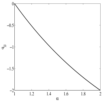
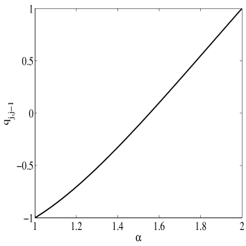
Figure 1: Coefficients (18): (a) $q_{jj}$ (b) $q_{j,j-1}$

  

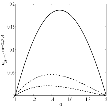
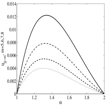
Figure 2: Coefficients (18): (a) $q_{j,j-m}$, $m=2,3,4$; (b) $q_{j,j-m}$, $m=5,6,7,8$

The following lemma characterizes the coefficients $q_{j,j-m}$ and is useful to prove our next results.

Lemma 4

Consider the coefficients $q_{j,j-m}$ defined by (18). Then

(a) $q_{j,j+1}=1,\quad$ $q_{j,j}\leq 0,\quad$ $q_{j,j-m}\geq 0,\ m\geq 2,\quad$ $\displaystyle{\lim_{m\rightarrow\infty}}q_{j,j-m}=0\quad$ and $q_{j,j-(m+1)}\leq q_{j,j-m}\leq q_{j,j-2}$.

(b) $\displaystyle{\sum_{m=2}^{\infty}}q_{j,j-m}=-3+3\times 2^{3-\alpha}-3^{3-\alpha}$.

(c) $\displaystyle{\sum_{m=-1}^{\infty}}q_{j,j-m}=0$.

Proof : (a) We have that $q_{j,j+1}=a_{j,j}=1$, $q_{j,j}=2^{3-\alpha}-4\leq 0$, for $1<\alpha\leq 2$ and $q_{j,j-1}=3^{3-\alpha}-4\times 2^{3-\alpha}+6$, which can be positive or negative depending on the value of $\alpha$. The $q_{j,j-m}$, $m\geq 2$, are of the form

$$q_{j,j-m}=(m+2)^{3-\alpha}-4(m+1)^{3-\alpha}+6m^{3-\alpha}-4(m-1)^{3-\alpha}+(m-2)^{3-\alpha}.$$

Hence,

$$q_{j,j-m}={}$$ (46)

$$m^{3-\alpha}\left[\left(1+\frac{2}{m}\right)^{3-\alpha}-4\left(1+\frac{1}{m}\right)^{3-\alpha}+6-4\left(1-\frac{1}{m}\right)^{3-\alpha}+\left(1-\frac{2}{m}\right)^{3-\alpha}\right]{}$$

$$= m^{3-\alpha}\left[\sum_{k=0}^{\infty}\left(\begin{array}[]{c}3-\alpha\\ k\end{array}\right)\left(\frac{2}{m}\right)^{k}-4\sum_{k=0}^{\infty}\left(\begin{array}[]{c}3-\alpha\\ k\end{array}\right)\left(\frac{1}{m}\right)^{k}+6\right.{}$$

$$\left.-4\sum_{k=0}^{\infty}\left(\begin{array}[]{c}3-\alpha\\ k\end{array}\right)\left(\frac{-1}{m}\right)^{k}+\sum_{k=0}^{\infty}\left(\begin{array}[]{c}3-\alpha\\ k\end{array}\right)\left(\frac{-2}{m}\right)^{k}\right]{}$$

leading to

$$q_{j,j-m} = m^{3-\alpha}\left[\sum_{k=4}^{\infty}\left(\begin{array}[]{c}3-\alpha\\ k\end{array}\right)\left(\frac{2}{m}\right)^{k}-4\sum_{k=4}^{\infty}\left(\begin{array}[]{c}3-\alpha\\ k\end{array}\right)\left(\frac{1}{m}\right)^{k}\right.{}$$

$$\left.-4\sum_{k=4}^{\infty}\left(\begin{array}[]{c}3-\alpha\\ k\end{array}\right)\left(\frac{-1}{m}\right)^{k}+\sum_{k=4}^{\infty}\left(\begin{array}[]{c}3-\alpha\\ k\end{array}\right)\left(\frac{-2}{m}\right)^{k}\right]{}$$

$$= m^{3-\alpha}\left[\frac{(3-\alpha)(3-\alpha-1)(3-\alpha-2)(3-\alpha-3)}{4!}\frac{24}{m^{4}}+\dots\right]{}$$

$$= \frac{1}{m^{\alpha-1}}\left[\frac{(3-\alpha)(2-\alpha)(1-\alpha)(-\alpha)}{4!}\frac{24}{m^{2}}+\dots\right].$$ (57)

Considering (57) and noting that the $k$ odd terms of the series cancel, the properties (a) can be easily obtained.

(b) In order to compute the series, let us first compute the sum of the first $M-1$ terms. We have

$${\sum_{m=2}^{M}}q_{j,j-m}=-3+3\times 2^{3-\alpha}-3^{3-\alpha}+s_{M},$$

where

$$s_{M}=-(M-1)^{3-\alpha}+3M^{3-\alpha}-3(M+1)^{3-\alpha}+(M+2)^{3-\alpha}.$$

Similar to what is done in (a) we can write

$$s_{M} = M^{3-\alpha}\left[\left(1+\frac{2}{M}\right)^{3-\alpha}-3\left(1+\frac{1}{M}\right)^{3-\alpha}+3-\left(1-\frac{1}{M}\right)^{3-\alpha}\right]{}$$ (65)

$$= M^{3-\alpha}\left[\sum_{k=0}^{\infty}\left(\begin{array}[]{c}3-\alpha\\ k\end{array}\right)\left(\frac{2}{M}\right)^{k}-3\sum_{k=0}^{\infty}\left(\begin{array}[]{c}3-\alpha\\ k\end{array}\right)\left(\frac{1}{M}\right)^{k}+3\right.{}$$

$$\left.-\sum_{k=0}^{\infty}\left(\begin{array}[]{c}3-\alpha\\ k\end{array}\right)\left(\frac{-1}{M}\right)^{k}\right].{}$$

Therefore

$$s_{M} = M^{3-\alpha}\left[\sum_{k=3}^{\infty}\left(\begin{array}[]{c}3-\alpha\\ k\end{array}\right)\left(\frac{2}{M}\right)^{k}-3\sum_{k=3}^{\infty}\left(\begin{array}[]{c}3-\alpha\\ k\end{array}\right)\left(\frac{1}{M}\right)^{k}\right.{}$$

$$\left.-\sum_{k=3}^{\infty}\left(\begin{array}[]{c}3-\alpha\\ k\end{array}\right)\left(\frac{-1}{M}\right)^{k}\right]{}$$

$$= M^{3-\alpha}\left[\frac{(3-\alpha)(2-\alpha)(1-\alpha)}{3!}\frac{6}{M^{3}}+\dots\right]{}$$

$$= \frac{1}{M^{\alpha-1}}\left[\frac{(3-\alpha)(2-\alpha)(1-\alpha)}{3!}\frac{6}{M}+\dots\right].$$ (74)

Clearly, we can conclude that $\lim_{M\rightarrow\infty}s_{M}=0$. Hence,

$$\sum_{m=2}^{\infty}q_{j,j-m}=\lim_{M\rightarrow\infty}\sum_{m=2}^{M}q_{j,j-m}=-3+3\times 2^{3-\alpha}-3^{3-\alpha}.$$

(c) This result comes immediately from (b) and from the fact that $q_{j,j+1}+q_{j,j}+q_{j,j-1}=3-3\times 2^{3-\alpha}+3^{3-\alpha}$.

Remark: Note that, the previous result lead us to conclude the series, defining the operator (19), converges absolutely when we have a bounded function $u$.

The next theorem states the method is unconditionally stable for $\tau\in[1/2,1]$.

Theorem 5

The weighted numerical method (23) is unconditionally von Neumann stable for $\tau\in[1/2,1]$.

Proof: Let us insert the mode $\kappa^{n}{\rm e}^{ij\theta}$ into (36). We obtain the following

$$\kappa^{n+1}(\theta)\left[{\rm e}^{ij\theta}-\tau\frac{\mu^{\alpha}}{\Gamma(4-\alpha)}\sum_{m=-1}^{\infty}q_{j,j-m}{\rm e}^{i(j-m)\theta}\right]$$

$$=\kappa^{n}(\theta)\left[{\rm e}^{ij\theta}+(1-\tau)\frac{\mu^{\alpha}}{\Gamma(4-\alpha)}\sum_{m=-1}^{\infty}q_{j,j-m}{\rm e}^{i(j-m)\theta}\right].$$

The amplification factor is given by

$$\kappa(\theta)\left[1-\tau\frac{\mu^{\alpha}}{\Gamma(4-\alpha)}\sum_{m=-1}^{\infty}q_{j,j-m}{\rm e}^{-im\theta}\right]=\left[1+(1-\tau)\frac{\mu^{\alpha}}{\Gamma(4-\alpha)}\sum_{m=-1}^{\infty}q_{j,j-m}{\rm e}^{-im\theta}\right].$$

Therefore $|\kappa(\theta)|\leq 1$ if and only if the real part of the series is negative, that is,

$$\sum_{m=-1}^{\infty}q_{j,j-m}\cos(m\theta)\leq 0,$$

since the imaginary part of the right side is smaller for $\tau\in[1/2,1]$, because $\tau\geq 1-\tau$. We can write

$$\sum_{m=-1}^{\infty}q_{j,j-m}\cos(m\theta) = (q_{j,j+1}+q_{j,j-1})\cos(\theta)+q_{j,j}{}$$ (75)

$$+\sum_{m=2}^{\infty}q_{j,j-m}\cos(m\theta).$$

Since $q_{j,j+1}+q_{j,j-1}\geq 0,$ and $q_{j,j-m}\geq 0$ for $m\geq 2$,

$$\sum_{m=-1}^{\infty}q_{j,j-m}\cos(m\theta) \leq (q_{j,j+1}+q_{j,j-1})+q_{j,j}+\sum_{m=2}^{\infty}q_{j,j-m}.$$ (76)

Now using Lemma 3. (c), we obtain

$$\sum_{m=-1}^{\infty}q_{j,j-m}\cos(m\theta) \leq 0.$$ (77)

$\square$

4 Matricial form

We start to describe the matricial form of the numerical method, taking in consideration that to implement the numerical method we need to have a computational bounded domain. Let us assume we consider the computational domain $[a,b]$, where the mesh is defined as $x_{j}=a+j\Delta x$ and we assume we have

$$u(a,t)=0,\qquad\mbox{and}\qquad u(b,t)=g_{b}(t)\qquad\mbox{given}$$

It is straightforward to conclude, that if $u(a,t)=0$, the problem is equivalent to a problem defined in the whole real line with the solution zero for $x\leq a$.

The numerical method can be written in the matricial form

$$\left(I-\tau\frac{\mu^{\alpha}}{\Gamma(4-\alpha)}Q\right){\bf U}^{n+1} = \left(I+(1-\tau)\frac{\mu^{\alpha}}{\Gamma(4-\alpha)}Q\right){\bf U}^{n}{}$$ (78)

$$+\frac{\mu^{\alpha}}{\Gamma(4-\alpha)}\left(\tau{\bf b}^{n+1}+(1-\tau){\bf b}^{n}\right)+{\bf p}^{n+\tau},$$

where $\qquad{\bf p}^{n+\tau}=\left[\Delta t\tau p_{1}^{n+1}+(1-\tau)p_{1}^{n}\dots\Delta t\tau p_{N-1}^{n+1}+(1-\tau)p_{N-1}^{n}\right]^{T}$,
${\bf U}^{n}=\left[U_{1}^{n}\dots U_{N-1}^{n}\right]^{T}$, ${\bf b}^{n}$ contains the boundary values, $\mu^{\alpha}$ is a diagonal matrix with entries $\mu_{j}^{\alpha}$ and $Q$ is related to the fractional operator. The matrix $Q=[Q_{j,k}]$ has the following structure

$$Q_{j,k}=\left\{\begin{array}[]{ll}q_{j,k},&1\leq k\leq j-1\\ q_{j,j},&k=j\\ q_{j,j+1},&k=j+1\\ 0,&k>j+1.\end{array}\right.$$

Finally the vector ${\bf b}^{n}$ is given by

$${b}_{j}^{n}=\left\{\begin{array}[]{ll}0,&j=1,\dots,N-2\\ q_{j,j+1}U_{N}^{n},&j=N-1.\end{array}\right.$$

assuming that $U_{0}^{n}=0$ and $U_{N}^{n}=g_{b}(t_{n})$.

Remark: From Lemma 4, for $q_{j,j-1}\geq 0$ (i.e. $\alpha>1.5545$), we can also easily prove our numerical method is unconditionally stable by the Gerschgorin’s theorem applied to the iterative matrix.

5 Numerical implementation

The numerical experiments are carried out in two parts. First, we verify the accuracy and order of convergence of the numerical method to confirm the theoreticall results presented in the previous sections. Then a physical application is considered to reveal some of the physical phenomena, from anomalous to mormal diffusion.

Consider the vectors $U_{app}(\Delta x)=(U_{0},\dots,U_{N})$, where $U_{j}$ is the approximate solution, for $x_{j}=x_{0}+j\Delta x$, $j=0,\dots,N$ at a certain time $t$, and $u_{ex}(\Delta x)=(u(x_{0},t),\dots,u(x_{N},t))$, where $u$ is the exact solution. The error is defined by the $l_{\infty}$ norm as,

$$||u_{ex}(\Delta x)-U_{app}(\Delta x)||_{\infty}=\max_{0\leq j\leq N}\left|u(x_{j},t)-U_{j}\right|.$$ (79)

Example 1. Consider the problem with initial condition $u(x,0)=4x^{2}(2-x)^{2}$, $0<x<2$ and zero otherwise. Let

$$d(x)=\frac{1}{4}\Gamma(5-\alpha)x^{\alpha},$$ (80)

and

$$p(x,t)=-4{\rm e}^{-t}x^{2}\left[7(2-x)^{2}+2\alpha(\alpha-7)+6x\alpha\right].$$ (81)

The exact solution is given by $u(x,t)=4{\rm e}^{-t}x^{2}(2-x)^{2}$, for $0\leq x\leq 2$, and zero otherwise.

In Table 1, we show the behaviour of the error (79) for different values of $\tau$ and for $\Delta t=\Delta x=1/30$ for the problem (80)–(81).

$\tau$	$\alpha=1.2$	$\alpha=1.4$	$\alpha=1.5$	$\alpha=1.8$
0.5	4.0277$\times 10^{-3}$	3.4191$\times 10^{-3}$	3.1944$\times 10^{-3}$	2.4542$\times 10^{-3}$
0.6	5.6194$\times 10^{-3}$	4.9682$\times 10^{-3}$	4.7877$\times 10^{-3}$	4.2856$\times 10^{-3}$
0.7	7.5094$\times 10^{-3}$	6.7573$\times 10^{-3}$	6.5920$\times 10^{-3}$	6.2510$\times 10^{-3}$
0.8	9.5429$\times 10^{-3}$	8.6634$\times 10^{-3}$	8.4903$\times 10^{-3}$	8.2598$\times 10^{-3}$
0.9	1.1656$\times 10^{-2}$	1.0625$\times 10^{-2}$	1.0435$\times 10^{-2}$	1.0283$\times 10^{-2}$
1.0	1.3814$\times 10^{-2}$	1.2615$\times 10^{-2}$	1.2403$\times 10^{-2}$	1.2318$\times 10^{-2}$

Table 1: Global $l_{\infty}$ error (79) of time converged solution at  $t=1$   for  $\alpha=1.2$,  $\alpha=1.4$,  $\alpha=1.5$,  $\alpha=1.8$ and $\Delta t=\Delta x=1/30$.

The most accurate result is for $\tau=1/2$. For the same problem, we observe in Table 2 and Table 3 that for all values of $\alpha$ we have second order convergence as expected, when $\tau=1/2$.

$\Delta x$	$\alpha=1.2$	Rate	$\alpha=1.4$	Rate
1/5	1.5310$\times 10^{-1}$		1.1950$\times 10^{-1}$
1/10	3.6239$\times 10^{-2}$	2.0789	3.0270$\times 10^{-2}$	1.9811
1/20	9.0506$\times 10^{-3}$	2.0015	7.6627$\times 10^{-3}$	1.9820
1/40	2.2669$\times 10^{-3}$	1.9973	1.9289$\times 10^{-3}$	1.9901

Table 2: Global $l_{\infty}$ error (79)of time converged solution for four mesh resolutions at $t=1$ for $\alpha=1.2,\alpha=1.4$, $\Delta t=\Delta x$ and $\tau=1/2$.

$\tau$	$\alpha=1.5$	Rate	$\alpha=1.8$	Rate
1/5	1.0884$\times 10^{-1}$		7.9651$\times 10^{-2}$
1/10	2.8101$\times 10^{-2}$	1.9535	2.0820$\times 10^{-2}$	1.9357
1/20	7.1358$\times 10^{-3}$	1.9775	5.4174$\times 10^{-3}$	1.9423
1/40	1.8050$\times 10^{-3}$	1.9831	1.3974$\times 10^{-3}$	1.9549

Table 3: Global $l_{\infty}$ error (79) of time converged solution for four mesh resolutions at $t=1$ for $\alpha=1.5,\alpha=1.8$, $\Delta t=\Delta x$ and $\tau=1/2$.

Example 2. Consider now a second problem with initial condition $u(x,0)=x^{\lambda}$, $0\leq x\leq 1$ and boundary conditions $u(0,t)=0$ and $u(1,t)={\rm e}^{-t}$. Let

$$d(x)=\frac{\Gamma(\lambda+1-\alpha)}{\Gamma(\lambda+1)}x^{\alpha+1}\quad\mbox{and}\quad p(x,t)=-(1+x){\rm e}^{-t}x^{\lambda}.$$ (82)

The exact solution of the problem is of the form

$$u(x,t)={\rm e}^{-t}x^{\lambda},\qquad x\in[0,1].$$ (83)

Although this problem is not defined in the whole real line we have $u(0,t)=0$, and this can be seen as a problem for which the solution is zero when $x\leq 0$.

In Table 4, we show the behavior of the error (79) for different weighted coefficients $\tau$. We observe the most accurate behaviour is again for $\tau=1/2$.

$\tau$	$\alpha=1.2$	$\alpha=1.4$	$\alpha=1.5$	$\alpha=1.8$
0.5	6.4792$\times 10^{-5}$	2.9402$\times 10^{-5}$	1.7850$\times 10^{-5}$	4.0509$\times 10^{-6}$
0.6	9.6854$\times 10^{-4}$	7.0639$\times 10^{-4}$	6.2104$\times 10^{-4}$	4.5122$\times 10^{-4}$
0.7	1.8609$\times 10^{-3}$	1.3815$\times 10^{-3}$	1.2233$\times 10^{-3}$	9.0545$\times 10^{-4}$
0.8	2.7426$\times 10^{-3}$	2.0533$\times 10^{-3}$	1.8233$\times 10^{-3}$	1.3587$\times 10^{-3}$
0.9	3.6143$\times 10^{-3}$	2.7219$\times 10^{-3}$	2.4211$\times 10^{-3}$	1.8110$\times 10^{-3}$
1.0	4.4769$\times 10^{-3}$	3.3870$\times 10^{-3}$	3.0166$\times 10^{-3}$	2.2624$\times 10^{-3}$

Table 4: Global $l_{\infty}$ error (79) of time converged solution for the problem (82) calculated by weighted numerical scheme with $\Delta t=\Delta x=1/30,\lambda=3,0\leq x\leq 1$ for different values of $\alpha$ and $\tau$.

In Table 5 we present a comparison between our method and the methods presented in [16] with the same space and time steps. The second column shows the absolute value of the largest error calculated by the Crank-Nicolson scheme (before extrapolation) presented in [16] at time $t=1.0$ which consists of assuming the fractional derivative is approximated by the shifted Grünwald-Letnikov formula. The third column shows the error calculated by the Crank-Nicolson scheme after a Richardson’s extrapolation presented in [16]. The fourth column shows the largest absolute error for our numerical scheme with $\tau=0.5$. Note that our numerical results are more accurate than the method given in [16].

$\Delta x$	CN-GL [16]	Extrapolated CN-GL [16]	Weighted ($\tau=0.5$)
1/10	1.82265$\times 10^{-3}$	1.77324$\times 10^{-4}$	3.5504$\times 10^{-5}$
1/15	1.16803$\times 10^{-3}$	7.85366$\times 10^{-5}$	1.6197$\times 10^{-5}$
1/20	8.64485$\times 10^{-4}$	4.40627$\times 10^{-5}$	9.1072$\times 10^{-6}$
1/25	6.84895$\times 10^{-4}$	2.82750$\times 10^{-5}$	5.8030$\times 10^{-6}$

Table 5: Global $l_{\infty}$ error (79) of time converged solution for the second problem calculated at $t=1$ for the second problem with $\Delta t=\Delta x,\lambda=3,0\leq x\leq 1$ and $\alpha=1.8$.

To conclude this example we observe the rate of convergence of the numerical method for different values of $\tau\neq 1/2$. The expected convergence rate for $\tau\neq 1/2$ according to section 3 is $O(\Delta t+\Delta x^{2})$. We consider $\Delta t=\Delta x^{2}$ to get second order convergence as we observe in Table 6.

	$\Delta t$	$\Delta x$	$\alpha=1.8$	Rate
	1/25	1/5	7.9325$\times 10^{-4}$	-
$\tau=0.6$	1/100	1/10	2.1501$\times 10^{-4}$	1.8834
	1/400	1/20	5.3710$\times 10^{-5}$	2.0011
	1/1600	1/40	1.3512$\times 10^{-5}$	1.9909
	1/25	1/5	1.2837$\times 10^{-3}$	-
$\tau=0.7$	1/100	1/10	3.5212$\times 10^{-4}$	1.8662
	1/400	1/20	8.7892$\times 10^{-5}$	2.0023
	1/1600	1/40	2.2053$\times 10^{-5}$	1.9948
	1/25	1/5	1.7723$\times 10^{-3}$	-
$\tau=0.8$	1/100	1/10	4.8915$\times 10^{-4}$	1.8573
	1/400	1/20	1.2207$\times 10^{-4}$	2.0026
	1/1600	1/40	3.0594$\times 10^{-5}$	1.9964
	1/25	1/5	2.2590$\times 10^{-3}$	-
$\tau=0.9$	1/100	1/10	6.2608$\times 10^{-4}$	1.8513
	1/400	1/20	1.5624$\times 10^{-4}$	2.0026
	1/1600	1/40	3.9134$\times 10^{-5}$	1.9973
	1/25	1/5	2.7438$\times 10^{-3}$	-
$\tau=1.0$	1/100	1/10	7.6292$\times 10^{-4}$	1.8466
	1/400	1/20	1.9041$\times 10^{-4}$	2.0024
	1/1600	1/40	4.7674$\times 10^{-5}$	1.9978

Table 6: Global $l_{\infty}$ error (79) of time converged solution for the numerical scheme (23) at $t=1$, for $\Delta t=\Delta x^{2}$ and $\alpha=1.8$, $\lambda=3$ and different values of $\tau$.

Example 3. Finally, in order to reveal the dynamics behavior of the diffusion equation (1), in this example we consider equation (1) without the source function (which means $p(x,t)=0$) on a finite domain $[0,4]$. We consider the Gaussian function

$$u(x,0)=\frac{1}{\sigma\sqrt{2\pi}}\exp(-\frac{(x-2)^{2}}{2\sigma^{2}})$$

as the initial condition, the diffusion coefficient $d(x)=1$ and the boundary conditions $u(0,t)=u(4,t)=0.$ The numerical results for this example are calculated by the weighted scheme with $\tau=1/2$. In this test, we take $\sigma=0.01$. The evolution of the non-Fickian diffusion processes for different values of $\alpha$ are given in Fig 3. The anomalous diffusion parameter exhibits the extent of the long tail diffusion processes of problem (1). The non-Fickian behavior gradually disappear when $\alpha\rightarrow 2$. This is consistent with the experimental results [1, 7, 13, 14]. Again the validity of our numerical methods is confirmed.

(a) $\alpha=1.4$                                            (b) $\alpha=1.6$

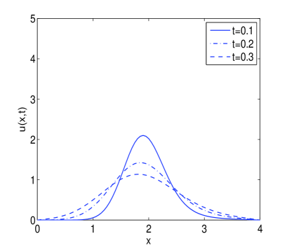
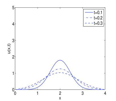
(c) $\alpha=1.8$                                            (d) $\alpha=1.999$

Figure 3: The evolution of $u(x,t)$ for different anomalous diffusion coefficients $\alpha$ at different times.

6 Conclusions

We have derived a weighted numerical method for the fractional diffusion equation based on the Riemann-Liouville derivative defined in an unbounded domain. The numerical method is second order accurate for $\tau=1/2$ and first order accurate for $\tau\in(1/2,1]$ because of the time discretization. We have proved theoretically the method converges by showing consistency and von Neumann stability. In the end we have presented test problems which are in agreement with the theoretical results.

References

- [1] D.A. Benson, S.W. Wheatcraft, M.M. Meerschaert, Application of a fractional advection-dispersion equation, Water Resour. Res. 36 (2000) 1403–1412.
- [2] D.A. Benson, R. Schumer, S.W. Wheatcraft, and M.M. Meerschaert, Fractional dispersion, Lévy motion, and the MADE tracer tests, Transp. Porous Media 42 (2001), 211-240.
- [3] W.H. Deng, C. Li, Finite difference methods and their physical constraints for the fractional Klein–Kramers equation, Numer. Methods Partial Differential Equations, in press (doi:10.1002/ num.20596).
- [4] K Diethelm, N.J. Ford, A.D. Freed, Detailed error analysis for a fractional Adams method, Numer. Algorithms 36 (2004) 31–52.
- [5] V.J. Ervin and J.P. Roop, Variational formulation for the stationary fractional advection dis persion equation, Numer. Methods Partial Differential Equations, 22 (2006), 558–576.
- [6] R. Gorenflo, F. Mainardi, Fractional calculus and stable probability distributions, Arch. Mech. 50 (1998) 377-388.
- [7] G. Huang, Q. Huang, H. Zhan, Evidence of one-dimensional scale-dependent fractional advection-dispersion, J. Contam. Hydrol. 85 (2006) 53–71.
- [8] C. Li, C. Tao, On the fractional Adams method, Comput. Math. Appl. 58, (2009) 1573 – 1588.
- [9] F. Liu, V. Ahn, and I. Turner, Numerical solution of the space fractional Fokker-Planck equation, J. Comput. Appl. Math., 166 (2004), 209-219.
- [10] V.E. Lynch, B.A. Carreras, D. del-Castillo-Negrete, K.M. Ferreira-Mejias and H.R. Hicks, Numerical methods for the solution of partial differential equations of fractional order, J. Comput. Phys., 192 (2003), 406-421.
- [11] R. Metzler, J. Klafter, The random walk’s guide to anomalous diffusion: a fractional dynamics approach, Phys. Rep. 339 (2000) 1–77.
- [12] R. Metzler, J. Klafter, Accelerating Brownian motion: a fractional dynamics approach to fast diffusion, Europhys. Lett. 51 (2000) 492–498.
- [13] Y. Pachepsky, D. Benson, W. Rawls, Simulating scale-dependent solute transport in soils with the fractional advective-dispersive equation, Soil Sci. Soc. Am. J. 4 (2000) 1234–1243.
- [14] L. Zhou, H.M. Selim, Application of the fractional advection-dispersion equation in porous media, Soil Sci. Soc. Am. J. 67 (2003) 1079–1084.
- [15] S. Shen, F. Liu, Error analysis of an explicit finite difference approximation for the space fractional diffusion equation with insulated ends, ANZIAM J. 46 (E) (2005) C871-C887.
- [16] C. Tadjeran, M.M. Meerschaert, H-P Scheffler, A second-order accurate numerical approximation for the fractional diffusion equation, J. Comput. Physics 213 (2006) 205–213.
- [17] A.A. Kilbas, H.M. Srivastava, J.J. Trujillo, Theory and Applications of Fractional Differential equations, Elsevier, 2006.
- [18] M.M. Meerschaert, C. Tadjeran, Finite difference approximations for fractional advection-dispersion flow equations, J. Comput. Appl. Math. 172 (2004) 65–77.
- [19] M.M. Meerschaert, C. Tadjeran, Finite difference approximations for two-sided space-fractional partial differential equations, Applied Numerical Mathemathics 56 (2006) 80–90.
- [20] K.S. Miller, B. Ross, An introduction to the fractional calculus and fractional differential equations. Wiley, New York, 1993.
- [21] K.B. Oldham and J. Spanier, The fractional calculus. Academic Press, New York, 1974.
- [22] I. Podlubny, Fractional Differential Equations, Academic Press, San Diego, 1999.
- [23] M.J.D. Powell, Approximation theory and methods, Cambridge University Press, Cambridge, 1981.
- [24] S.G. Samko, A.A. Kilbas, O.I. Marichev, Fractional Integrals and derivatives: theory and Applications, Gordon and Breach Science Publishers, 1993.
- [25] E. Sousa, Finite difference approximations for a fractional advection diffusion problem, J. Comput. Phys., 228 (2009) 4038 – 4054.
- [26] E. Sousa, Numerical approximations for fractional diffusion equations via splines, Comput. Math. Appl. doi:10.1016/j.camwa.2011.04.015.
- [27] L. Su, W. Wang and H. Wang, A characteristic finite difference method for the transient fractional convection-diffusion equations, Applied Numerical Mathematics, 61, (2011), 946–960.
- [28] R. Schumer, D.A. Benson, M.M. Meerschaert, S.W. Wheatcraft, Eulerian derivation of the fractional advection-dispersion equation J. Contam. Hydrol., 48 (2001) 69-88.
- [29] G.M. Zaslavsky, Chaos, fractional kinetics, and anomalous transport, Phys. Rep. 371 (2002) 461-–580.
- [30] S.B. Yuste, L. Acedo, An explicit finite difference method and a new von Neumann–type stability analysis for fractional diffusion equations, SIAM J. Numer. Anal. 42 (2005) 1862–1874.
- [31] X. Zhang, M.Lv Mouchao, J.W. Crawford and I.M. Young, The impact of boundary on the fractional advection-dispersion equation for solute transport in soil: Defining the fractional dispersive flux with Caputo derivatives, Adv. Water Resour. 30 (2007) 1205–1217.