A Weakly nonlinear theory for spiral density waves excited by accretion disc turbulence

Abstract

We develop an analytic theory to describe spiral density waves propagating in a shearing disc in the weakly nonlinear regime. Such waves are generically found to be excited in simulations of turbulent accretion disks, in particular if said turbulence arises from the magneto-rotational instability (MRI). We derive a modified Burgers equation governing their dynamics, which includes the effects of nonlinear steepening, dispersion, and a bulk viscosity to support shocks. We solve this equation approximately to obtain nonlinear sawtooth solutions that are asymptotically valid at late times. In this limit, the presence of shocks is found to cause the wave amplitude to decrease with time as $t^{-2}$. The validity of the analytic description is confirmed by direct numerical solution of the full nonlinear equations of motion. The asymptotic forms of the wave profiles of the state variables are also found to occur in MRI simulations indicating that dissipation due to shocks plays a significant role apart from any effects arising from direct coupling to the turbulence.

1 Introduction

Accretion discs are common in astrophysics, occurring in close binary systems, active galactic nuclei and around protostars where they provide the environment out of which planets form (see e.g. Papaloizou & Lin, 1995; Lin & Papaloizou, 1996, for reviews).

Observational inferred accretion rates require enhanced angular momentum transport to take place. This is believed to be mediated by some form of turbulence, which can be regarded as providing an effective anomalous viscosity. The most likely source of accretion disk turbulence is the magneto-rotational instability (MRI, see Balbus & Hawley, 1991, 1998).

In both local and global simulations of the MRI with and without net magnetic flux, prolific density wave excitation has been found (e.g. Gardiner & Stone (2005) in the local case, and Armitage (1998) in the global case). Such waves may be important in the contexts of quasi periodic oscillations. They may also be associated with stochastic migration of protoplanets (Nelson & Papaloizou, 2004; Nelson, 2005) and with providing some residual angular momentum transport in magnetically inactive dead zones Gammie (1996).

In view of the significance of these waves it is important to gain an understanding of the processes leading to their excitation and ultimate dissipation. In Heinemann & Papaloizou (2009a) we developed a WKBJ theory for the excitation of these density waves in the linear regime and found that vortensity fluctuations are responsible for their excitation during a short period of time, as they change from being leading to trailing, denoted as swing. In a second paper (Heinemann & Papaloizou, 2009b), we studied the wave excitation process directly as it occurs in fully non-linear three dimensional numerical MRI simulations. The results were found to be in good agreement with the WKBJ description of the excitation process developed in Heinemann & Papaloizou (2009a).

In this paper we extend the work of our previous two papers to consider the behavior of the waves as they enter the nonlinear regime. This is significant because the eventual development of weak shocks is expected and this leads to the dissipation of the waves. Their maximum amplitude can be expected to be determined by a balance between excitation and dissipation processes. The latter might occur either directly through wave phenomena such as shocks, or through interaction with the turbulence. Possibilities here include energy loses resulting from random secondary density wave generation through interaction of the primary wave with turbulent eddies (e.g. Lighthill, 1953; Howe, 1971a, b; Ffowcs Williams & Howe, 1973). Another phenomenon that could potentially play a role is distortion of the primary wave front on account of a variable wave propagation speed caused by the presence of dynamic turbulent eddies (e.g. Hesselink & Sturtevant, 1988). Understanding these phenomena is notoriously difficult and their theoretical description is, at present, somewhat imprecise and associated with issues of interpretation. In the body of this paper we focus on weakly nonlinear wave theory without turbulence and defer consideration of wave-turbulence interactions until the discussion section.

Our studies, in common with the majority of those that incorporate turbulence resulting from the MRI, are restricted to local isothermal disc models. Accordingly they do not incorporate the possibility of the channeling of wave energy towards the upper disc layers, that may occur for density waves with short wavelengths in the direction of the shear, in models with significant thermal stratification (Ogilvie & Lubow, 1999).

As shown in Heinemann & Papaloizou (2009a, b), turbulent vortensity fluctuations are able to excite pairs of counter-propagating spiral density waves when they swing from leading to trailing. Subsequently, as the excited waves propagate, their wavelengths in the direction of propagation decrease and the conservation of wave momentum results in an increasing amplitude, causing them to enter the nonlinear regime in which the formation of shocks occurs. Our aim is to describe the time asymptotic form of these excited waves and the way in which the associated shock dissipation leads to amplitude decay, and to relate these phenomena to what is seen in MRI simulations.

We consider the nonlinear evolution of a single pair of counter-propagating spiral density waves on a homogeneous background. As we will demonstrate, this becomes an effectively one-dimensional problem when described in a shearing coordinate frame, reducing to ordinary one-dimensional gas dynamics in the far trailing regime.

The plan of the paper is as follows. In Section 2 we describe the shearing box model and present the basic equations. In Section 2.1 we introduce shearing coordinates, giving the form of the basic equations governing solutions that are functions only of the shearing coordinate in the direction of the shear and time. We go on to express these using a Lagrangian formalism in Section 2.2, deriving the appropriate forms of specific vorticity or vortensity conservation in Section 2.3, and nonlinear wave momentum conservation in Section 2.4.

In Section 3 we use the Lagrangian formulation as the basis for the development of an analytic description that is applicable to the weakly nonlinear regime. In this formulation, third order effects such as entropy production in shocks are neglected, making it possible to adopt an adiabatic or isothermal equation of state (e.g. Yano, 1996). In Section 3.1 we derive a modified Burgers equation governing the unidirectional propagation of weakly nonlinear waves (for a similar approach to the problem of nonlinear planetary wakes see Goodman & Rafikov, 2001). This is found to provide the correct nonlinear development of wave profiles in which weak shocks are ultimately present. Nonlinear sawtooth solutions, which are asymptotically valid at late times, are derived in Section 3.2. Corrections to the wave profile arising from dispersive effects are derived in Section 3.3.

In Section 4 we go on to present numerical solutions of the full nonlinear equations governing a pair of counter-propagating spiral density waves undergoing swing excitation. At late times these are compared with analytic solutions derived in Section 3.2. The form of the wave profiles and the decay of the wave amplitudes with time are found to be in excellent agreement. Finally in Section 5 we discuss our results, comparing them with what is seen in, and considering their consequences for, MRI simulations.

2 Model basic equations and preliminaries

We adopt the standard local shearing box of Goldreich & Lynden-Bell (1965) and assume that the effect of magnetic fields on the density waves we consider is negligible. The basic equations are the conservation of mass and momentum in the form

$$\frac{\partial{\rho}}{\partial{t}}+\nabla\cdot(\rho\mn@boldsymbol{v})=0$$ (1)

$$\frac{\partial{\mn@boldsymbol{v}}}{\partial{t}}+\mn@boldsymbol{v}\cdot\nabla\mn@boldsymbol{v}+2\mn@boldsymbol{\Omega}\times\mn@boldsymbol{v}=-\frac{\nabla P}{\rho}+2q\Omega^{2}x\mn@boldsymbol{e}_{x}+\mn@boldsymbol{f}.$$ (2)

Here $\rho$, $P$, $\mn@boldsymbol{v}$, and $\mn@boldsymbol{f}$ are the density, pressure, velocity, and viscous force per unit mass, respectively. We adopt a Cartesian coordinate system $(x,y,z)$ with origin at the center of the box. The $x$-direction points away from a putative central object, the $y$-direction is in the direction of rotation and the $z$-direction is parallel to the rotation axis. The unit vectors in these coordinate directions are $\mn@boldsymbol{e}_{x}$, $\mn@boldsymbol{e}_{y}$, and $\mn@boldsymbol{e}_{z}$ respectively. The angular velocity of the system is $\mn@boldsymbol{\Omega}=\Omega\mn@boldsymbol{e}_{z}$. For a Keplerian disk the constant $q=3/2$.

In order to complete the description, we require an equation of state. This may be found by noting that the pressure $P$ can be taken to be a function of the density $\rho$ and the entropy per unit mass $S$. From the first and second laws of thermodynamics, the entropy satisfies the equation

$$T\left(\frac{\partial{S}}{\partial{t}}+\mn@boldsymbol{v}\cdot\nabla S\right)=\epsilon,$$ (3)

where $T$ is the temperature and $\epsilon$ is the net rate of heating per unit mass. When the latter is zero – as we will assume throughout this paper – then the motion is adiabatic, with $S$ being conserved on a fluid element, and we may write $S=S_{0}$, where $S_{0}$ is the fixed entropy per unit mass. We point out that heating by shocks will, in general, cause departures from an adiabatic equation of state, even in the absence of cooling. However, such effects enter only at third order in the wave amplitude (e.g. Yano, 1996) and hence do not affect the dynamics of weakly nonlinear waves of the type considered in this paper.

The basic state on which the waves we eventually consider propagate is such that $P$, $\rho$ and $S$ are constant and the velocity $\mn@boldsymbol{v}=-q\Omega{}x\mn@boldsymbol{e}_{y}$. Then for adiabatic motion $S_{0}$ is constant and the relation $P=P(\rho,S_{0})$ leads to an effectively barotropic equation of state. We neglect vertical gravity and thermal stratification and look for waves that have no dependence on $z$. We note, however, that in the strictly isothermal case ($P\propto\rho$), the velocity amplitudes associated with the density waves we consider turn out not to depend on $z$ even if the disk is vertically structured (Fromang & Papaloizou, 2007). But note that this situation could be modified for density waves with short wavelength in the direction of the shear if the disc model were to have significant thermal stratification (Ogilvie & Lubow, 1999).

2.1 Shearing coordinates

In the theory of linear wave excitation developed in Heinemann & Papaloizou (2009a, b) the coordinate dependence of the asymptotic form of the excited waves at late times is through an exponential factor

$$\exp\bigl{[}\mathrm{i}k_{y}(y+q\Omega tx)+\mathrm{i}k_{x}x\bigr{]},$$

where $k_{y}$ is the constant azimuthal wavenumber and $k_{x}$ is the radial wavenumber at $t=0$. This latter quantity can be removed by redefining the origin of time to correspond to the time at which the wave swings from leading to trailing. Thus without loss of generality we may take $k_{x}$ to be zero.

When we go on to study the nonlinear development of the waves, it is natural to consider disturbances with the same coordinate dependence as described above. It is accordingly convenient to transform to shearing coordinates $(x^{\prime},y^{\prime})$, which are related to $(x,y)$ through

$$x^{\prime}=x,\ y^{\prime}=y+q\Omega xt.$$ (4)

The shearing coordinate $y^{\prime}$ specifies the coordinate of an unperturbed fluid element in the direction of the background flow, being $y$ at the reference time $t=0$. It is also convenient to work in terms of the velocity perturbation to the background shear $\mn@boldsymbol{u}=\mn@boldsymbol{v}+q\Omega{}x\mn@boldsymbol{e}_{y}$. Then, in shearing coordinates, the coordinate dependence is on $y^{\prime}$ alone, so that equations (1) and (2) become

$$\left.\frac{\partial{\rho}}{\partial{t}}\right|_{y^{\prime}}+\frac{\partial{}}{\partial{y^{\prime}}}\Bigl{[}\rho(u_{y}+q\Omega tu_{x})\Bigr{]}=0$$ (5)

and

$$\left.\frac{\partial{\mn@boldsymbol{u}}}{\partial{t}}\right|_{y^{\prime}}+(u_{y}+q\Omega tu_{x})\frac{\partial{\mn@boldsymbol{u}}}{\partial{y^{\prime}}}+2\mn@boldsymbol{\Omega}\times\mn@boldsymbol{u}-q\Omega u_{x}\mn@boldsymbol{e}_{y}=$$

$$-\left(\frac{\mn@boldsymbol{e}_{y}+q\Omega t\mn@boldsymbol{e}_{x}}{\rho}\right)\frac{\partial{P}}{\partial{y^{\prime}}}+\mn@boldsymbol{f},$$ (6)

where we have indicated that time derivatives are to be taken at constant $y^{\prime}$.

2.2 Lagrangian description

Equations (5) and (2.1) describe a form of gas dynamics in one spatial dimension. For such problems a simplification can often be made by adopting a Lagrangian description that uses a spatial coordinate that remains fixed on a fluid element. Such a coordinate, $y_{0}(y^{\prime},t)$, may be defined through the equation

$$\left.\frac{\partial{y^{\prime}}}{\partial{t}}\right|_{y_{0}}=u_{y}+q\Omega tu_{x}.$$ (7)

Following Lynden-Bell & Ostriker (1967), we introduce an undisturbed ’ghost’ flow, which in the present case is simply the background shear flow. We consider the mapping of fluid elements from the disturbed flow to the ghost flow and take $y_{0}$ to be the initial value of $y^{\prime}$ for the corresponding element of the ghost flow. We remark that with this specification we do not require that $y^{\prime}$ for the disturbed flow and $y_{0}$ coincide at time $t=0$ which in turn allows for a non zero density perturbation at $t=0$. Note that (7) states that $y^{\prime}$ moves with the component of fluid velocity normal to the phase surfaces of constant $y^{\prime}$.

It is convenient to work in terms of the specific volume $V=1/\rho$. Conversion of the spatial variable from $y^{\prime}$ to $y_{0}$ is effected by using the relation

$$\frac{\partial{y^{\prime}}}{\partial{y_{0}}}=\frac{\rho_{0}}{\rho}=\frac{V}{V_{0}},$$ (8)

which follows from (5) and (7). Here, $\rho_{0}$ is the uniform background density, which is fixed for a given fluid element and $V_{0}=1/\rho_{0}$. In the Lagrangian description equations (5) and (2.1) thus transform to

$$\left.\frac{\partial{V}}{\partial{t}}\right|_{y_{0}}=V_{0}\frac{\partial{(u_{y}+q\Omega tu_{x})}}{\partial{y_{0}}},$$ (9)

$$\left.\frac{\partial{u_{x}}}{\partial{t}}\right|_{y_{0}}-2\Omega u_{y}=-q\Omega tV_{0}\frac{\partial{P}}{\partial{y_{0}}}+f_{x},$$ (10)

$$\left.\frac{\partial{u_{y}}}{\partial{t}}\right|_{y_{0}}+(2-q)\Omega u_{x}=-V_{0}\frac{\partial{P}}{\partial{y_{0}}}+f_{y}.$$ (11)

2.3 Vortensity conservation

An equation for the evolution of the ratio of the vertical component of vorticity to the density, which we refer to as the ‘vortensity’, is obtained from equations (10) and (11) by multiplying the latter by $q\Omega t$ and subtracting it from the former. With the help of equation (9) we then obtain

$$\frac{\partial{Q}}{\partial{t}}+V_{0}\frac{\partial{(f_{x}-q\Omega tf_{y})}}{\partial{y_{0}}}=0,$$ (12)

where the vortensity is given by

$$Q=(2-q)\Omega V+V_{0}\frac{\partial{(q\Omega tu_{y}-u_{x})}}{\partial{y_{0}}},$$ (13)

and from now on we omit to indicate that time derivatives are taken at constant $y_{0}$. We also find it convenient to separate specific volume and the vortensity into background and perturbed parts according to $V=V_{0}+\delta{}V$ and $Q=Q_{0}+\delta{}Q$, respectively, where $Q_{0}=(2-q)\Omega/\rho_{0}$ is the background vortensity and

$$\delta Q=(2-q)\Omega\delta V+V_{0}\frac{\partial{(q\Omega tu_{y}-u_{x})}}{\partial{y_{0}}}$$ (14)

is the vortensity perturbation. We remark that in the inviscid case, equation (12) shows that vortensity is strictly conserved on fluid elements. This remains true when viscous forces arise from a bulk viscosity, as can be easily seen by noting that in this case the viscous forces can be taken into account as an addition to the pressure. Furthermore, equation (12) is in conservation law form. In Eulerian form this reads

$$\left.\frac{\partial{\left(\rho Q\right)}}{\partial{t}}\right|_{y^{\prime}}+{\partial\over\partial y^{\prime}}\bigl{[}\rho Q(u_{y}+q\Omega tu_{x})+(f_{x}-q\Omega tf_{y})\bigr{]}=0.$$

It implies that vortensity is conserved across shocks for any kind of small viscosity (even though it may not be conserved in passing trough the shock width). Thus for infinitesimal viscosity we may adopt $\delta{}Q=0$ everywhere and apply the standard Rankine-Hugoniot conditions to determine the changes to other quantities on passing through shocks. Note that this is only valid for planar shocks, which we are considering here. Curved shocks are in general associated with vortensity production (see e.g. Hayes, 1957).

In this context we note that in the linear theory of wave excitation described in Heinemann & Papaloizou (2009a), vortensity perturbations in the form of stationary waves play a vital role in that excitation of traveling spiral density waves only occurs if such perturbations are present. Wave excitation happens during a narrow time interval around $t=0$ (the time of the swing), at which point a pair of counter-propagating spiral density waves linearly couples to a stationary vortical wave. However, this coupling is not effective at later times due to an increasing frequency mismatch between the vortical wave and the spiral density waves, so that we may take $\delta Q=0$ when describing the dynamics of the latter at late times.

2.4 Conservation of wave momentum in the nonlinear regime

It is also possible to formulate the conservation of wave momentum for motions governed by equations (9) to (11). To do this we introduce the Lagrangian displacement through

$$\frac{\partial{\mn@boldsymbol{\xi}}}{\partial{t}}=-q\Omega\xi_{x}\mn@boldsymbol{e}_{y}+\mn@boldsymbol{u}.$$ (15)

The Lagrangian displacement $\mn@boldsymbol{\xi}=(\xi_{x},\xi_{y})$ is measured relative to the background or ‘ghost’ fluid introduced in Section 2.2 and is not necessarily small. In terms of it, equations (10) and (11) are given by

$$\frac{\partial^{2}{\xi_{x}}}{\partial{t}^{2}}-2\Omega\frac{\partial{\xi_{y}}}{\partial{t}}-2q\Omega^{2}\xi_{x}=-q\Omega tV_{0}\frac{\partial{P}}{\partial{y_{0}}}+f_{x},$$ (16)

$$\frac{\partial^{2}{\xi_{y}}}{\partial{t}^{2}}+2\Omega\frac{\partial{\xi_{x}}}{\partial{t}}=-V_{0}\frac{\partial{P}}{\partial{y_{0}}}+f_{y},$$ (17)

and a time integration of equation (9) yields

$$\delta V=V_{0}\frac{\partial{(\xi_{y}+q\Omega t\xi_{x})}}{\partial{y_{0}}}.$$ (18)

Having expressed the equations of motion in terms of Lagrangian displacement, we can now derive a conservation law for wave momentum in the form of

$$\frac{\partial{\mathcal{U}}}{\partial{t}}+\frac{\partial{\mathcal{F}}}{\partial{y_{0}}}=-\mn@boldsymbol{f}\cdot\frac{\partial{\mn@boldsymbol{\xi}}}{\partial{y_{0}}},$$ (19)

where the wave momentum density is

$$\mathcal{U}=-\left(\frac{\partial{\mn@boldsymbol{\xi}}}{\partial{t}}+\mn@boldsymbol{\Omega}\times\mn@boldsymbol{\xi}\right)\cdot\frac{\partial{\mn@boldsymbol{\xi}}}{\partial{y_{0}}}$$ (20)

and the associated flux is

$$\mathcal{F}=-P\delta V+\mathcal{L}.$$ (21)

Here, $\mathcal{L}$ is the Lagrangian density for the system in the absence of dissipative forces. This is given by

$$\mathcal{L}=\frac{1}{2}\frac{\partial{\mn@boldsymbol{\xi}}}{\partial{t}}\cdot\frac{\partial{\mn@boldsymbol{\xi}}}{\partial{t}}+(\mn@boldsymbol{\Omega}\times\mn@boldsymbol{\xi})\cdot\frac{\partial{\mn@boldsymbol{\xi}}}{\partial{t}}+q\Omega^{2}\xi_{x}^{2}-E,$$ (22)

where $E(V,S)$ is the internal energy, to which the pressure is related by

$$P=-\left.\frac{\partial{E}}{\partial{V}}\right|_{S}.$$ (23)

When there are no dissipative forces, equation (19) is a strict conservation law that implies that the wave momentum flux $\mathcal{F}$ is constant in a steady state. We remark that this discussion does not necessarily require a uniform background. It applies when $V_{0}$ is not constant and to the adiabatic case with $S_{0}$ not constant. By considering the effect of external forces the flux $\mathcal{F}$ is found to be a momentum flux that converts to an angular momentum flux on multiplication by an assumed radius of the center of the box.

When dissipation is included wave momentum is no longer conserved. From the discussion in Section 2.3 it is apparent that we can investigate the role of shocks by including a bulk viscosity. This can be done by adding a component $\Pi$ to the pressure given by

$$\Pi=-\frac{\zeta}{V^{2}}\frac{\partial V}{\partial t},$$ (24)

where $\zeta$ is the coefficient of bulk viscosity. In this form it is clear that this adds a positive contribution to the pressure when the gas is being compressed, as is required to support shocks. The viscous force corresponding to (24) is given by

$$\mn@boldsymbol{f}=-(q\Omega t\mn@boldsymbol{e}_{x}+\mn@boldsymbol{e}_{y})V_{0}\frac{\partial{\Pi}}{\partial{y_{0}}}.$$ (25)

When a bulk viscosity is included in this way, equation (19) is modified to read

$$\frac{\partial{\mathcal{U}}}{\partial{t}}+\frac{\partial{(\mathcal{F}-\Pi\delta V)}}{\partial{y_{0}}}=-\Pi\frac{\partial{V}}{\partial{y_{0}}}.$$ (26)

Thus, wave momentum is no longer conserved.

The right hand side of (26) is in fact related to the local rate of dissipation of energy per unit mass, given by

$$\epsilon=-\Pi\frac{\partial{V}}{\partial{t}}.$$ (27)

Accordingly, the right hand side of equation (26) may be re-expressed as $\epsilon(\partial{}V/\partial{}t)^{-1}\partial{}V/\partial{}y_{0}$. For a non-dispersive traveling wave, the quantity multiplying $\epsilon$ is simply $-1/v_{0}$, where $v_{0}$ is the wave velocity in the shearing coordinate $y_{0}$. Let us consider an outward (inward) propagating trailing wave, traveling in the direction of increasing (decreasing) $y_{0}$, for which $v_{0}>0$ ($v_{0}<0$). As is well known, such a wave carries a positive (negative) amount of momentum. Equation (26) thus implies that the momentum content of each wave is lost to the background. This is consistent with both waves being associated with an outward momentum flux.

3 Weakly nonlinear theory

Although we are considering sheared disturbances with a specific coordinate dependence (see Section 2.1), we have so far not made any further approximations. In this section we now restrict our consideration to waves with finite but sufficiently small amplitude so that all terms of higher than quadratic order in the wave amplitude can be neglected. We will also generally consider the waves to be in the far trailing regime.

We start by noting that the number of dynamical equations that describe nonlinear spiral density waves can be reduced to just a pair of equations by invoking vortensity conservation. Indeed, we can dispose of the dynamical equation for $u_{y}$ by using (14) to express this quantity in terms of $u_{x}$, $\delta{}V$, and $\delta{}Q$. As we discussed in the end of Section 2.3, we may set the vortensity perturbation $\delta{}Q=0$, in which case

$$u_{y}=\frac{1}{q\Omega t}\left[u_{x}+\frac{(q-2)\Omega\,\partial_{y_{0}}^{-1}\delta V}{V_{0}}\right].$$ (28)

Here, $\partial_{y0}^{-1}$ denotes the inverse of the partial derivative with respect to $y_{0}$. An arbitrary function of time arising from the integration with respect to $y_{0}$ is left unspecified at this point. We will later determine this by enforcing momentum conservation (see Section 3.3 below). A consequence of (28) is that in the limit of late times, the characteristic magnitude of $u_{y}$ is smaller than that of $u_{x}$ by a factor of $q\Omega t$. In this limit, it is convenient to adopt the quadratic time variable

$$\tau=\frac{q\Omega t^{2}}{2},$$ (29)

in terms of which the equations of motion governing the nonlinear waves are given by

$$\frac{\partial{V}}{\partial{\tau}}=V_{0}\left(\frac{\partial{u_{x}}}{\partial{y_{0}}}+\frac{1}{q\Omega t}\frac{\partial{u_{y}}}{\partial{y_{0}}}\right)$$ (30)

$$\frac{\partial{u_{x}}}{\partial{\tau}}=\frac{V_{0}c^{2}}{V^{2}}\frac{\partial{V}}{\partial{y_{0}}}+\frac{2\Omega u_{y}}{q\Omega t}-V_{0}\frac{\partial{\Pi}}{\partial{y_{0}}}.$$ (31)

Here, we recall that recall that $c^{2}=-V^{2}\partial{}P/\partial{}V$ evaluated at constant entropy is the square of the sound speed and it is understood that $t=\sqrt{2\tau/q\Omega}$.

In the limit of large $\tau$ and vanishing viscosity, equations (30) and (31) become equivalent to the standard equations for gas dynamics. The terms involving $u_{y}$ lead to small corrections that arise from the non-uniformity of the shearing medium through which the waves propagate. In the linear theory given in Heinemann & Papaloizou (2009a), they are seen to induce slow amplitude and phase changes occurring on a time scale long compared to the inverse wave frequency. These effects appear at first order in a WKBJ treatment and we shall treat additional changes arising from nonlinearity and viscosity on the same footing below.

The asymptotic similarity to one-dimensional gas dynamics described in the previous paragraph suggests that we describe the nonlinear waves using the Riemann invariants

$$R_{\pm}=u_{x}\pm\int^{V}_{V_{0}}\frac{c\,\mathrm{d}V}{V},$$ (32)

in terms of which the equations of motion are given by

$$\frac{\partial{R_{\pm}}}{\partial{\tau}}=\pm\frac{cV_{0}}{V}\frac{\partial{}}{\partial{y_{0}}}\left(R_{\pm}+\frac{u_{y}}{q\Omega t}\right)+\frac{2\Omega u_{y}}{q\Omega t}-V_{0}\frac{\partial{\Pi}}{\partial{y_{0}}}.$$ (33)

We note that this pair of equations is still exact. Independently of wave amplitude, in the limit of both large $\tau$ and small $\zeta$, they have solutions consisting of simple waves. These are such that the forward propagating wave has $R_{+}=0$ and the backward propagating wave has $R_{-}=0$. The propagation speed $cV_{0}/V$ corresponds to a propagation speed $c$ when measured with respect to the Eulerian coordinate $y^{\prime}$. In the linear approximation the general solution is a superposition of simple waves.

3.1 An approximate wave equation governing weakly nonlinear waves

At leading order in WKBJ theory, the Riemann invariants satisfy first order linear wave equations, according to which $R_{\pm}$ travel in opposite directions at constant amplitude with speed $c_{0}$, being the sound speed $c$ evaluated for $V=V_{0}$. We consider modifications to the leading order dynamics resulting from weak nonlinearity in the wave amplitudes $R_{\pm}$, corrections resulting from the presence of $u_{y}$ at large $\tau$, as well as corrections resulting from a small amount of viscosity. As the last two corrections are intrinsically small, we only consider them to linear order.

To express quantities of interest in terms of the Riemann invariants, we note that $u_{x}=(R_{+}+R_{-})/2$ and $\int^{V}_{V_{0}}(c/V)\,\mathrm{d}V=(R_{+}-R_{-})/2$. From these two relations it follows that if we set $V=V_{0}+\delta{}V$, then to first order in the wave amplitude $\delta{}V$ we have $c_{0}\delta{}V/V_{0}\approx(R_{+}-R_{-})/2$. Recalling that $c_{0}$ is the sound speed evaluated for $V=V_{0}$, the propagation speed is, to the same level of accuracy, given by

$$\frac{cV_{0}}{V}\approx c_{0}-\left(\frac{\delta V}{V_{0}}\right)c_{1}\approx c_{0}-\left(\frac{R_{+}-R_{-}}{2}\right)\frac{c_{1}}{c_{0}},$$ (34)

where

$$c_{1}=-V_{0}^{2}\frac{\partial{(c/V)}}{\partial{V}}\Big{|}_{V=V_{0}}.$$ (35)

Note that $c_{1}=c_{0}$ for an isothermal equation of state.

We focus on the forward propagating wave, which to leading order in WKBJ theory is described by $R_{-}$ (a corresponding parallel analysis can be done for the backward propagating wave). In the dynamical equation for $R_{-}$, the terms containing $u_{y}$ and $\Pi$ (which, as remarked above, we consider to be linear) as well as the weakly nonlinear contribution due to the variable wave speed, given by (34), involve both $R_{-}$ and $R_{+}$. However, it is possible to argue that $R_{+}$ may be neglected in the equation for $R_{-}$. We can see this from the following considerations.

Assuming that the forward propagating wave is dominated by $R_{-}$, we can estimate $R_{+}$ from its dynamical equation, which has small terms proportional to $R_{-}$ as sources. In the rest frame of $R_{-}$, these source terms appear to be of high frequency because $R_{+}$ travels in the opposite directions. This leads to the conclusion that the induced $R_{+}$ will be small compared to the original $R_{-}$ and so its contribution to the small terms in the equation for $R_{-}$ may be neglected. We note that such a situation is common in weakly nonlinear hyperbolic systems, see Hunter & Keller (1983) for a general treatment.

With $R_{+}$ dropped and terms involving $u_{y}$ and $\Pi$ treated as linear, the equation for $R_{-}$ becomes

$$\frac{\partial{R_{-}}}{\partial{\tau}}+\left(c_{0}+\frac{c_{1}}{2c_{0}}R_{-}\right)\frac{\partial{R_{-}}}{\partial{y_{0}}}=\hskip 85.35826pt$$

$$-\frac{1}{q\Omega t}\left(c_{0}\frac{\partial{u_{y}}}{\partial{y_{0}}}-2\Omega u_{y}\right)-V_{0}\frac{\partial{\Pi}}{\partial{y_{0}}},$$ (36)

where $u_{y}$ and $\Pi$, respectively defined in (28) and (24), are to first order in small quantities given by

$$u_{y}=\frac{1}{2q\Omega t}\Bigl{[}R_{-}+(2-q)\Omega(c_{0}\partial_{y_{0}})^{-1}R_{-}\Bigr{]}$$ (37)

and

$$\Pi=\frac{1}{2}(2q\Omega\tau)^{1/2}\frac{\zeta}{V_{0}c_{0}}\frac{\partial{R_{-}}}{\partial{\tau}}.$$ (38)

In the last expression for the viscous pressure, we consider the bulk viscosity coefficient $\zeta$ to be a small quantity, in which case we may replace $\partial{}R_{-}/\partial\tau$ by $-c_{0}\partial{}R_{-}/\partial{}y_{0}$.

The two terms on the right hand side of (37) give rise to various, qualitatively different effects when this expression is substituted into (3.1). Both terms lead to slow changes in the wave amplitude. The first term also leads to a modification of the propagation speed. The second term also introduces dispersion. All of these effects are consistent with linear WKBJ theory.

The change in the propagation speed is taken care of by transforming to a frame moving with speed

$$\left(1+\frac{1}{4q\Omega\tau}\right)c_{0}$$

in the $y_{0}$ direction. The new spatial coordinate is thus

$$\eta=y_{0}-c_{0}\int\left(1+\frac{1}{4q\Omega\tau}\right)\mathrm{d}\tau.$$ (39)

Finally, for notational convenience, we introduce

$$U=\frac{c_{1}}{2c_{0}}R_{-}.$$ (40)

The governing equation for waves propagating in the $y_{0}$ direction is then

$$\frac{\partial{U}}{\partial{\tau}}+U\frac{\partial{U}}{\partial{\eta}}-\frac{U}{4\tau}=\hskip 128.0374pt$$

$$\frac{\kappa^{2}(c_{0}\partial_{\eta})^{-1}U}{4q\Omega\tau}+\frac{1}{2}(2q\Omega\tau)^{1/2}\frac{\partial{}}{\partial{\eta}}\left(\zeta\frac{\partial{U}}{\partial{\eta}}\right),$$ (41)

where it is understood that $\partial/\partial\tau$ is now to be evaluated at constant $\eta$. At this point we remark that as indicated above, a parallel analysis can be performed to obtain the corresponding equation for the backward propagating wave described by $U=c_{1}R_{+}/(2c_{0})$. This is the same as (3.1), but with the sign of the dispersive term (first term on the right hand side) reversed. Its solutions may be obtained from those of (3.1) by use of the transformation $\eta\rightarrow-\eta$, $y_{0}\rightarrow-y_{0}$, $U\rightarrow-U$.

Note that the viscous term increases in magnitude as $\tau$ increases as a consequence of the shear causing the radial wavelength of the disturbance to shorten with time. The bulk viscosity coefficient $\zeta$ thus needs to decrease with time if the relative importance of the viscous term is not to change. The particular form of $\zeta$ that we use in Section 4 to integrate the equation of motion numerically has in fact this property.

Equation (3.1) may be viewed as a modified form of Burgers equation. The first two terms on the right hand side correctly account for first order changes in amplitude and phase arising in WKBJ theory. The only nonlinearity comes from the advection term on the left hand side, which causes wave steepening and the formation of shocks.

3.2 Nonlinear sawtooth waves

It is possible to consider solutions of equation (3.1) with different ordering regimes for the different terms. We have just discussed the case where nonlinear, dispersive and dissipative effects are all small. Physically this corresponds to a short wavelength wave in the linear regime with a conserved wave momentum which has not had time enough to steepen and form shocks. We now go on to consider the case when the nonlinear term dominates the dispersive and dissipative terms corresponding to a situation where the wave is in the process of forming a shock. Setting $\bar{U}=U/\tau^{1/4}$, adopting a new time coordinate $\bar{\tau}=(4/5)\,\tau^{5/4}$ and neglecting dispersive and dissipative terms on the right hand side of (3.1), this equation is transformed to the inviscid Burgers equation

$$\frac{\partial{\bar{U}}}{\partial{\bar{\tau}}}+\bar{U}\frac{\partial{\bar{U}}}{\partial{\eta}}=0.$$ (42)

It is a well known result in nonlinear acoustics that an initially monochromatic wave that satisfies Burgers equation steepens to form a sawtooth wave (see Parker, 1992, and references therein). Although we do not begin with a strictly monochromatic wave we are close to that situation and the numerical simulations of Section 4 show that the solutions to the full nonlinear equations of motion do in fact approach a sawtooth wave, so we shall consider these solutions here.

A sawtooth wave consists of a periodic array of shocks. Because we are considering the inviscid form of Burgers equation, we are implicitly taking the limit of vanishing viscosity. In this limit, the shocks in the sawtooth wave are infinitely thin and may be treated as discontinuities. The change in $\bar{U}$ is then determined from the conservation law associated with (42). For a stationary (i.e. non-traveling) wave, this requires that $\bar{U}$ changes sign across the shock.

The solution of (42) corresponding to a stationary sawtooth wave with wavelength $\lambda$ can be expressed in terms of $U$ as

$$U=\frac{5\eta}{4\tau}\,\frac{1}{1-(\tau_{0}/\tau)^{5/4}}$$ (43)

where the wave is periodically extended for $|\eta|>\lambda/2$ and $\tau_{0}$ is an arbitrary integration constant. The wavelength $\lambda$ (which we remark is time-independent when measured with respect to the shearing coordinate $y_{0}$) may be specified arbitrarily (but see below). The solution is linear in $\eta$ between a periodic array of shocks with amplitude $\lambda{}U/\eta$.

Noting that $u_{x}=c_{0}U/c_{1}$ and using the definitions of $\tau$ to express the result in terms of the time $t$, we see that for the fundamental period of the sawtooth wave, when $t$ and $\tau$ are large enough that $\tau_{0}$ may be neglected, we have

$$u_{x}=\frac{c_{0}}{2c_{1}}\frac{5\eta}{q\Omega t^{2}}.$$ (44)

The maximum velocity amplitude is obtained by setting $\eta=\lambda/2$. The wavelength $\lambda$ thus determines the shock amplitude at a given late time. The fact that this amplitude decays implies dissipation of energy, which may be interpreted as being due to the action of a vanishingly small bulk viscosity within an infinitely thin shock layer. As we discussed in Section 2.4, dissipation of energy is always associated with angular momentum transfer to the background.

3.3 Correction for dispersion

We now estimate corrections to the sawtooth solution resulting from dispersion but still take viscosity to be vanishingly small. We work in the limit of large $\tau$ so that again $\tau_{0}$ in (43) is neglected. The governing equation is equation (3.1) with $\zeta=0$ which reads

$$\frac{\partial{U}}{\partial{\tau}}+U\frac{\partial{U}}{\partial{\eta}}-\frac{U}{4\tau}=\frac{\kappa^{2}(c_{0}\partial_{\eta})^{-1}U}{4q\Omega\tau}$$ (45)

We begin by allowing for a small change to the time dependent propagation speed of the wave, which we are regarding to be of the same order as the correction we are estimating. This gives us the freedom to ensure that the correct jump conditions across the shock are maintained. We thus add a term $c_{2}(\tau){\partial{}U}/{\partial\eta}$ to both sides of (45), where $c_{2}(\tau)$ is the as yet undefined small increase in the propagation speed. In order to deal with the additional term on the left hand side, we redefine the co-moving coordinate $\eta$ so that it is boosted by the speed $c_{2}(\tau)$ and thus given by

$$\eta=y_{0}-c_{0}\int\left(1+\frac{1}{4q\Omega\tau}\right)\mathrm{d}\tau-\int\!c_{2}(\tau)\,\mathrm{d}\tau.$$ (46)

In terms of the new co-moving coordinate, equation (45) becomes

$$\frac{\partial{U}}{\partial{\tau}}+U\frac{\partial{U}}{\partial{\eta}}-\frac{U}{4\tau}=\frac{\kappa^{2}(c_{0}\partial_{\eta})^{-1}U}{4q\Omega\tau}+c_{2}(\tau)\frac{\partial{U}}{\partial{\eta}},$$ (47)

where we emphasize again that the last term on the right hand side is supposed to lead to a small correction of the same order as that produced by the first term on the right hand side.

To find an approximate solution we set $U=U_{0}+U_{1}$ where $U_{0}$ is the sawtooth solution given by (43) and $U_{1}$ is a small correction. Dropping terms that are quadratic in $U_{1}$ on the left hand side of (47), and neglecting $U_{1}$ on the right hand side, we find that $U_{1}$ satisfies the equation

$$\frac{\partial{U_{1}}}{\partial{\tau}}+\frac{5\eta}{4\tau}\frac{\partial{U_{1}}}{\partial{\eta}}+\frac{U_{1}}{\tau}=\frac{\kappa^{2}}{4q\Omega\tau}\left[\frac{5\eta^{2}+g(\tau)}{8c_{0}\tau}\right]$$ (48)

Here, $g(\tau)$ is an arbitrary function arising partly from the operator $\partial_{\eta}^{-1}$ and partly from the incorporation of the last term on the right hand side of (47). It can be chosen to ensure that at any time the wave has no mean momentum, i.e.

$$\int_{-\lambda/2}^{\lambda/2}(U_{0}+U_{1})\,\mathrm{d}\eta=0.$$ (49)

To solve (48) we set $U_{1}(\eta,\tau)=\alpha(\tau)\eta^{2}+\beta(\tau)$. The functions $\alpha(\tau)$ and $\beta(\tau)$ can be found by substituting this ansatz into (48) and integrating with respect to $\tau$. In fact, one has only to find $\alpha(\tau)$, since $\beta(\tau)$ can then be determined using the constraint (49). The dispersive correction is thereby found to be

$$U_{1}(\eta,\tau)=\frac{\kappa^{2}(\eta^{2}-\lambda^{2}/12)}{16q\Omega\tau c_{0}}.$$ (50)

We now turn to the evaluation of $c_{2}(\tau)$, which we introduced so as to ensure that the correct shock jump conditions are satisfied. From (47) it is apparent that

$$U^{2}/2-c_{2}U\approx U_{0}^{2}/2+U_{0}(U_{1}-c_{2})$$

should be conserved when passing through the shock. Since $U_{0}$ changes sign across the shock and $U_{1}$ does not, this leads to

$$c_{2}(\tau)=U_{1}(\lambda/2,\tau)=\frac{\kappa^{2}\lambda^{2}}{96q\Omega\tau c_{0}}.$$ (51)

The corresponding correction to the co-moving coordinate defined in (46) is thus proportional to $\ln\tau$ and hence small.

In order to measure the modification of the sawtooth form due to the dispersive correction, we evaluate

$$\mathcal{R}=\left(\frac{\int_{-\lambda/2}^{\lambda/2}U_{1}^{2}\,\mathrm{d}\eta}{\int_{-\lambda/2}^{\lambda/2}U_{0}^{2}\,\mathrm{d}\eta}\right)^{1/2}=\frac{\kappa^{2}\lambda}{20\sqrt{15}\,q\Omega c_{0}}.$$ (52)

Interestingly, this expression does not depend on time but only on the wavelength $\lambda$. The dependence on $\lambda$ is such that the dispersive correction to the sawtooth is small for sufficiently short wavelengths. However, even for $\lambda=2\pi{}c_{0}/\Omega$, which is the optimal wavelength for excitation by vortensity fluctuations in a Keplerian disk (Heinemann & Papaloizou, 2009a), we find $\mathcal{R}=\pi/15^{3/2}\approx{}0.054$, suggesting that dispersive corrections to the sawtooth profile may be neglected in practice.

4 Numerical Simulations

We have obtained solutions of the set of nonlinear equations (9) to (11) by means of numerical simulations. In the limit $t\rightarrow\infty$ this set of equations leads to a pair of equations that resembles the standard equations for one dimensional inviscid gas dynamics with $\tau=q\Omega{}t^{2}/2$ as the effective time variable. As with those, we expect nonlinear wave steepening leading to the formation shock waves (e.g. Landau & Lifshitz, 1987). In order to represent these, viscous dissipation must be included. Although this has to be significant only in the thin transition region between the pre-shock and post-shock fluid. Here we deal with this by adopting the procedure of von Neumann & Richtmyer (1950) in which an artificial viscous pressure, $\Pi$, is added to the gas pressure, $P$. For the simulations presented here we adopt an isothermal equation of state, such that $P=c^{2}/V$, with the isothermal sound speed $c=c_{0}$ being constant. Then equations (9) to (11) together with (25 become

$$\rho_{0}\frac{\partial{V}}{\partial{t}}=\frac{\partial{(u_{y}+q\Omega tu_{x})}}{\partial{y_{0}}},$$ (53)

$$\rho_{0}\left[\frac{\partial{u_{x}}}{\partial{t}}-2\Omega u_{y}\right]=-q\Omega t\frac{\partial{(c^{2}/V+\Pi)}}{\partial{y_{0}}},$$ (54)

$$\rho_{0}\left[\frac{\partial{u_{y}}}{\partial{t}}+(2-q)\Omega u_{x}\right]=-\frac{\partial{(c^{2}/V+\Pi)}}{\partial{y_{0}}}.$$ (55)

The form of the viscous pressure $\Pi$ is given by (24) as

$$\Pi=-\frac{\zeta}{V^{2}}\frac{\partial{V}}{\partial{t}},$$ (56)

where, following von Neumann & Richtmyer (1950), we take the bulk viscosity coefficient to be

$$\zeta=(\rho_{0}\beta\Delta y_{0})^{2}V\left|\frac{\partial{V}}{\partial{t}}\right|.$$ (57)

Here, $\Delta{}y_{0}$ is the computational grid spacing in $y_{0}$ and $\beta$ is a constant of order unity which can be adjusted to smear shocks over a fixed number of numerical grid points (typically between 3 and 5). We adopted $\beta=3$ in our simulations.

We remark that because $y_{0}$ is a shearing coordinate, shock widths measured with respect to $y_{0}$ increase linearly with time at late times. This can be seen as follows. Inserting (57) into (56), and using the fact that for an outgoing wave we have to lowest order

$$\frac{\partial{V}}{\partial{t}}=-q\Omega tc\frac{\partial{V}}{\partial{y_{0}}}$$ (58)

(see Section 3.1), we find

$$\Pi=-\frac{(\rho_{0}c\beta q\Omega t\Delta y_{0})^{2}}{V}\frac{\partial{V}}{\partial{y_{0}}}\left|\frac{\partial{V}}{\partial{y_{0}}}\right|.$$ (59)

This expression has an additional factor $(q\Omega t)^{2}$ as compared to a standard case in non shearing coordinates. Thus the shock width scales as $\beta{}q\Omega{}t\Delta{}y_{0}$, which indeed increases linearly with time. Note, however, that $y_{0}\sim{}q\Omega{}tx$ at late times, which means that the width of a shock remains fixed when measured with respect to $x$. Thus, an observer in the “unsheared” coordinate frame $(x,y)$ will, at late times, see a shock of constant width propagating in the $x$-direction.

In practice, artificial viscosity is only significant in regions of strong compression, where $\partial{}V/\partial{}t<0$. Thus, the viscous pressure $\Pi$ is often set to zero in regions of rarefaction, where $\partial{}V/\partial{}t>0$. In our simulations, steep gradients never occur in these latter regions, so that this makes little difference, and we have found empirically that slightly better results are obtained without this modification.

Simulations were carried out on an equally spaced computational grid in $y_{0}$ with typically 16384 grid points. We note that because of this rather high resolution, the increase of the shock widths as discussed above is not actually visible in the plots shown below. The computational domain was taken to be periodic with period $2\pi{}c/\Omega$, which equals the optimal wave length for wave excitation for a Keplerian rotation profile (Heinemann & Papaloizou, 2009a). In order to discretize the equations of motion, we have adopted the same staggered leapfrog scheme that was used in von Neumann & Richtmyer (1950). This scheme is second order accurate in space and time away from shocks, but effectively becomes only first order accurate (in space) in their vicinity.

4.1 Initial conditions

We start the numerical integration of (53) to (55) at a time corresponding to a couple of orbits before the swing. The initial condition consists of a stationary vortical wave of small amplitude. To derive this initial condition, we note that in the linear inviscid regime, this system of equations is – according to Heinemann & Papaloizou (2009a) – equivalent to the inhomogeneous second-order wave equations

$$\left[\frac{\partial^{2}{}}{\partial{t}^{2}}+(q^{2}\Omega^{2}t^{2}+1)k^{2}c^{2}+\kappa^{2}\pm 2q\Omega\mathrm{i}kc\right]\left(\frac{u_{x}}{c}\mp\frac{\delta V}{V_{0}}\right)$$

$$=\left(\mathrm{i}kc\mp 2\Omega\right)\rho_{0}\delta Q$$ (60)

and

$$\left[\frac{\partial^{2}{}}{\partial{t}^{2}}+(q^{2}\Omega^{2}t^{2}+1)k^{2}c^{2}+\kappa^{2}\right]\frac{u_{y}}{c}=-q\Omega t\mathrm{i}k_{y}c\,\rho_{0}\delta Q,$$ (61)

where $\delta{}V$, $u_{x}$, $u_{y}$, and the vortensity perturbation $\delta{}Q$ are assumed to vary harmonically in space as $\exp(\mathrm{i}k{}y_{0})$. We note that vortensity conservation implies that $\delta{}Q$ does not vary in time at linear order.

At early times before the swing, we may drop the double time derivative in (4.1) and (61) to obtain the slowly varying vortical wave solutions

$$\left(\frac{u_{x}}{c}\mp\frac{\delta V}{V_{0}}\right)=\frac{\left(\mathrm{i}kc\mp 2\Omega\right)\rho_{0}\delta Q}{(q^{2}\Omega^{2}t^{2}+1)k^{2}c^{2}+\kappa^{2}\pm 2q\Omega\mathrm{i}kc}$$ (62)

and

$$\frac{u_{y}}{c}=-\frac{q\Omega t\mathrm{i}k_{y}c\,\rho_{0}\delta Q}{(q^{2}\Omega^{2}t^{2}+1)k^{2}c^{2}+\kappa^{2}},$$ (63)

where it is understood that the real part of the right hand sides is to be taken.

We initialize the integration with the vortical wave solution (62) and (63) at $t=-4\pi/\Omega$, corresponding to two orbits before the swing. In this way we generate initial conditions that lead to a time dependent evolution that firstly reproduces the linear wave excitation phase described in Heinemann & Papaloizou (2009a), in which the vortical wave gives rise to the excitation of a pair of counter-propagating spiral density waves at $t=0$. Subsequent evolution causes the spiral density waves to enter the nonlinear regime considered in this paper and described analytically in Section 3 above.

We assume a Keplerian rotation profile by setting $q=3/2$. For the azimuthal wavenumber we choose $k=1/H$, where $H=c/\Omega$ is the putative density scale height. This corresponds to an azimuthal wavelength of $2\pi{}H$, which is the optimal wavelength for spiral density wave excitation (see Heinemann & Papaloizou, 2009a, for details). The amplitude of the vortensity perturbation $\delta{}Q$ we take to be $0.1\Omega/\rho_{0}$.

4.2 Numerical results

In Figure 1 we compare the time evolution of solutions to the nonlinear equations of motion (53) to (55) obtained using the artificial viscosity method with solutions of the linear wave equations (4.1) and (61). To make this comparison, we computed the $k=1/H$ Fourier components of the nonlinear solutions for $u_{x}$, $u_{y}$, and $\delta{}V$ (denoted respectively by $\hat{u}_{x}$, $\hat{u}_{y}$, and $\delta\hat{V}$), and plotted the result against the linear solutions.

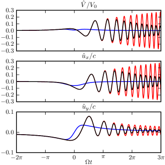
Figure 1: Evolution of the $k=1/H$ mode amplitudes according to the linear (red, attaining the largest values at late times) and nonlinear (black) equations of motion. The blue curves represent the corresponding vortical wave solutions (62) and (63). The linear solution was obtained by integrating the linearized equations of motion using a high order Runge-Kutta method.

The linear and nonlinear solutions are seen to agree closely during the leading phase $t<0$ and also during the early trailing phase $t>0$ after the wave excitation has taken place. This is consistent with the fact that the amplitude of the vortensity perturbation $\delta Q$ was chosen small enough to make the excitation process linear. Nonlinearity occurs later as the waves propagate. This is on account of the increasing amplitude implied as a consequence of wave momentum conservation (see Section 2.4 above). A consequence of nonlinearity and shock development is that the Fourier amplitudes $\hat{u}_{x}$ and $\delta\hat{V}$ do not continue to increase with time as predicted by the linear theory but instead attain maximum values and then decay. The maximum relative density perturbation is roughly 20%, which is attained at $t\sim{}3\pi/4\Omega$, is similar to that seen in nonlinear simulations of the MRI (Heinemann & Papaloizou, 2009b). It is interesting to note that although the nonlinear waves decay while the linear waves increase in amplitude they maintain the same phases at a given time. We will comment on this further below in Section 4.4.

The decay of the nonlinear wave amplitudes is due to a transfer of wave energy to smaller scales due to nonlinear mode coupling. That such energy transfer indeed occurs is illustrated in Figure 2 where we plot the specific volume $V$ as a function of $y_{0}$, over one wavelength, at three different times in the trailing phase. Already half an orbit after excitation, nonlinear steepening has lead to a notable distortion of the initial harmonic profile. After one orbit, further steepening has resulted in the formation of two shock fronts corresponding to the forward and backward propagating waves. These separate regions of almost constant specific volume. At this time the two shocks travel in opposite directions away from the central region. Yet another half of an orbit later, the spatial profile remains essentially unchanged, but the shock amplitudes have decreased by approximately a factor of two because of the energy dissipation associated with them.

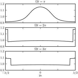
Figure 2: Spatial profile of the specific volume at different times in the trailing phase.

The spatial profiles of the velocity components and the specific volume perturbation three orbits after excitation are plotted in Figure 3. The shocks in the radial velocity $u_{x}$ are seen to be as pronounced as those in the relative specific volume perturbation $\delta{}V/V_{0}$. In this case they separate regions where the velocity varies almost linearly with $y_{0}$, corresponding to a sawtooth form. In comparison to $\delta{}V$ and $u_{x}$, the spatial variation in the azimuthal velocity field $u_{y}$ remains predominantly harmonic. As indicated in Figure 3, this sinusoidal variation corresponds to the non-oscillatory vortical wave solution that follows from (63). In contrast to this, the corresponding amplitudes obtained from (62) lead to negligibly small values of $\delta{}V/V_{0}$ and $u_{x}/c$. This suggests that in the case of $u_{y}$, the shock amplitude decays faster than the vortical wave amplitude, whereas the opposite seems to be the case for $\delta{}V$ and $u_{x}$. This is discussed further below.

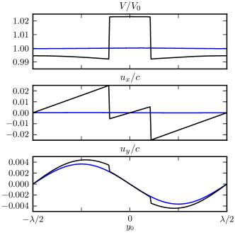
Figure 3: Spatial profiles of all fluid variables roughly three orbits after excitation ($\Omega{}t\approx 6\pi$). The black curve corresponds to the numerical solution. Also shown in blue are the corresponding vortical wave solutions (62) and (63).

4.3 Nonlinear damping

We note that when a forward propagating wave has attained a sawtooth form, equation (44), with $c_{0}=c_{1}=c$ which applies to the numerical simulations, gives $u_{x}$ as a function of the co-moving coordinate $\eta$ with a periodic extension for $|\eta|>\lambda/2$, with $\lambda$ being the azimuthal wave length of the original linear wave. The shock discontinuities are accordingly located at $\eta=(n+1/2)\lambda$, where $n{}\in\mathbb{Z}$ and the jump across the shock is given by

$$\Delta(u_{x})=\frac{5\lambda}{2q\Omega t^{2}}.$$ (64)

This applies to waves traveling in either direction as neither is preferred. Thus weakly nonlinear shock jumps decay quadratically in time. The decay of the shock amplitudes necessarily leads to a decay of the fluctuation energy per unit mass, defined as

$$\mathcal{E}=\frac{u_{x}^{2}+u_{y}^{2}}{2}+\frac{c^{2}}{V_{0}^{2}}\frac{\delta V^{2}}{2}.$$ (65)

Because for weakly nonlinear waves propagating in one direction, one of the Riemann invariants propagates while the other is constant, it follows that (64) gives the magnitude of the shock jump for both $u_{x}$ and $c\delta{}V/V_{0}$. From vortensity conservation, it follows that $u_{y}$ decays more rapidly than $\delta{}V$ and $u_{x}$ by one power of $t$ (see discussion in Section 3 above) and so may be dropped from (65) as $t\rightarrow\infty$. In this limit the fluctuation energy averaged over a wavelength associated with a pair of shock waves is given by

$$\langle\mathcal{E}\rangle=\frac{1}{6}\left(\frac{5\lambda}{2q\Omega t^{2}}\right)^{2}.$$ (66)

Thus the fluctuation energy at late time decays as $t^{-4}$.

We note that in the limit $t\rightarrow\infty$, the above description is ultimately independent of the initial wave amplitude. We have tested this inherently nonlinear expectation against the behavior of our numerical simulations. In Figure 4 we plot the fluctuation energy (65) for waves initiated with four different amplitudes of the vortensity perturbation $\delta{}Q$. According to the linear excitation mechanism described by Heinemann & Papaloizou (2009a), this amplitude, determines the amplitude of the excited linear wave. For the examples illustrated the fluctuation energies obtained shortly after excitation differ by almost two orders of magnitude. However, as $t$ approaches large values, the fluctuation energies associated with the numerical solutions all approach the predicted late-time fluctuation energy (66). This is because the more the initially linear wave is amplified, the sooner it becomes nonlinear, and larger amplitude waves decay faster than smaller amplitude ones.

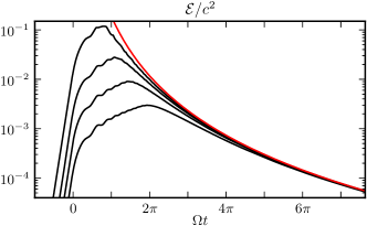
Figure 4: Time evolution of the fluctuation energy per unit mass $\mathcal{E}$, as defined by equation (65). Black curves not uppermost: Energy obtained numerically using the artificial viscosity method. Red and uppermost curve: Energy obtained from equation (66) obtained from weakly nonlinear theory, see Section 4.3.

4.4 Shock propagation

In this section we will investigate the space-time dependence of the nonlinear waves. We remind the reader that for the forward propagating weakly nonlinear solution described in Section 3.1, the co-moving coordinate is given by (46) as

$$\eta=y_{0}-c\tau-\frac{c\ln|\tau|}{4q\Omega}\left(1+\frac{\kappa^{2}\lambda^{2}}{24c^{2}}\right),$$ (67)

where we have now reverted back to quadratic time variable $\tau$ used in Section 3.1. For the backward propagating wave $c$ is replaced by $-c$ in (67). Apart from asymptotically insignificant amplitude (through $\lambda$) and logarithmic corrections, the functional form of the shock wave solution is the product of a time-dependent amplitude and a function of the phase $y_{0}-c\tau$ as is also the case for linear waves. Thus the speed at which the shock fronts propagate is approximately equal to the sound speed, being the phase speed of linear waves in the far trailing regime.

We are now in a position to understand the evolution of individual Fourier harmonics as obtained from the numerical solution of the nonlinear equations, as shown in Figure 1. There we see that while nonlinear effects do lead to a decrease in the oscillation amplitude, they do not seem to alter the oscillation period. This follows immediately from the fact that the linear and nonlinear waves maintain approximately the same phase as a function of time.

4.5 Shock wave profile

In Section 4.2 we illustrated the spatial profile of a pair of shock waves observed in a numerical simulation. This is characterized by a top-hat profile in the specific volume perturbation and a double sawtooth profile in the radial velocity. A similar double sawtooth profile is also seen in the azimuthal velocity, but there it is disguised by the spatially sinusoidal vorticity perturbation that we used as initial condition. As we will now demonstrate, all of these features can be understood from weakly nonlinear theory.

In Figure 5 we illustrate schematically the superposition of two counter-propagating sawtooth waves, corresponding to the weakly nonlinear asymptotic solutions derived in Section 3. The arrows indicated the direction of propagation. Note that the forward and backward propagating wave have the same slope. As we noted earlier, this is because the latter is obtained from the former by simultaneously reversing the sign of the wave amplitude and the spatial coordinate. Since the two sawtooth waves have the same slope, subtracting one from the other yields a top hat profile for the specific volume perturbation. Conversely, adding the two waves results in a double sawtooth profile for the radial velocity perturbation.

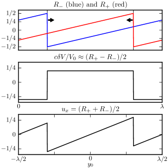
Figure 5: Sketch of the superposition of two counter-propagating sawtooth waves. The arrows indicated the direction of propagation. Note that the waves travel towards a region of low pressure (since $\delta{}p\sim 1/\delta{}V$).

We can gain additional confidence in the weakly nonlinear theory by testing it directly against the numerical data. In Figure 6, we plot analytic solutions on top of numerical solutions at a time corresponding to roughly three orbits after excitation. To achieve the best possible agreement, we have incorporated in the analytic solution both the dispersive correction to the sawtooth wave given by (50) as well as the stationary vortical wave that we used as initial condition.

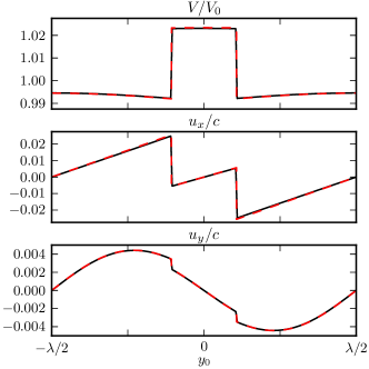
Figure 6: Comparison of wave forms roughly three orbits after excitation ($\Omega{}t\approx 6\pi$). Black: Numerical solution. Dotted red: Weakly nonlinear solution.

As Figure 6 shows, the analytic solutions are essentially indistinguishable from the numerical ones. We note that the only free parameter that enters the analytic solutions is the location of the shock front. The magnitude of the jump across the shock is in fact correctly predicted by (64). We also note that a superposition principle evidently holds. This confirms what we have argued for in Section 3.1, i.e. that weakly nonlinear, counter-propagating sawtooth waves do not interact to a good approximation.

Close inspection of the wave profile of the specific volume perturbation between shock fronts reveals that it is slightly curved. This curvature is a dispersive effect that is correctly captured by the dispersive correction to the leading order sawtooth solution. Unlike for $\delta{}V$, there is hardly any curvature in the wave profile of the radial velocity $u_{x}$. This is expected, as it turns out that the dispersive correction, which is quadratic in the spatial coordinate, enters $R_{+}$ and $R_{-}$ with opposite sign, so that it cancels out when their sum is taken to obtain $u_{x}$. We note that these effects cannot be attributed to the vortical wave as its amplitude is less than 1% of the shock amplitude. In addition, the curvature in the specific volume perturbation profile is everywhere concave. The vortical wave on the other hand would give rise to to a sinusoidal variation that is concave in one half of the domain and convex in the other.

Also illustrated in Figure 6 is the wave profile of the azimuthal velocity $u_{y}$. The analytic solution shown consists of a superposition of the vortical wave and the weakly nonlinear shock waves. The wave form is mostly sinusoidal, indicating that the vortical wave dominates. This is because in the case of $u_{y}$, the vortical wave decays as $t^{-1}$, whereas the shock waves decay as $t^{-3}$, so that the former will always dominate at late times.

For $\delta{}V$ and $u_{x}$, the vortical wave and the shock waves decay equally fast (as $t^{-2}$). In general, one might therefore expect to see the vortical wave at late times. Since this is not the case, we conclude that shortly after the initial wave excitation, the shock wave should be much larger in amplitude than the vortical wave. Inspection of Figure 1 shows that this is indeed the case.

5 Discussion and application to MRI simulations

We have considered the propagation of density waves in a shearing box. These were assumed to be functions only of the shearing coordinate $y+q\Omega xt$ and time $t$. The waves were presumed to have been excited by vortensity fluctuations produced by MRI turbulence as described by Heinemann & Papaloizou (2009a, b). In this process it is only the form of the vortensity fluctuation at the time when waves swing from being leading to trailing that is significant. Just after the swing inward and outward propagating waves are assumed, as found in simulations, to be in the linear regime. Subsequently, as the waves propagate, their wavelengths in the $x$ direction decreases, while the conservation of wave momentum results in increased amplitude, causing them to enter the nonlinear regime and the formation of shocks.

In Section 3 of this paper we developed an analytic theory that is applicable to the weakly nonlinear regime. We derived a modified Burgers equation governing the dynamics of weakly nonlinear waves, which contains terms describing nonlinear steepening, dispersion, and viscous diffusion. We obtained nonlinear sawtooth solutions with weak shocks valid for late times and estimated corrections resulting from dispersion.

In Section 4 we presented numerical solutions of the nonlinear equations without a small amplitude approximation. These led to sawtooth waves with a profile that was in excellent agreement with that obtained from the weakly nonlinear theory at late times, in particular with regard to rate of decay of the shock velocity jump being ultimately proportional to $t^{-2}$. The solutions constructed from the theory were composed of a combination of forward and backward propagating waves, resulting in a double sawtooth profile for the radial velocity $u_{x}$ and a top hat profile for the specific volume perturbation $\delta{}V$.

5.1 MRI simulations

An important issue is the extent to which the description of weakly nonlinear waves we have provided above applies to the density waves excited in MRI simulations. These waves are found to be ubiquitous in such simulations. As a typical example of what is found in many realizations we show in Figure 7 a snapshot of the (vertically integrated) mass and momentum densities found in a simulation described in Heinemann & Papaloizou (2009b). From this figure it is apparent that the wave structure is significantly more pronounced in $u_{x}$ and $\delta{}\rho/\rho_{0}\sim-\delta{}V/V_{0}$ than in the azimuthal velocity $u_{y}$. This is expected from our discussion in Section 4.2, which indicated that $u_{y}$ is dominated by the stationary vortical wave. In addition, Figure 7 indicates a top hat like profile in $\delta V$. To examine this more closely, Figure 8 shows plots of the fluid variables taken at a fixed value of $x$. These may be compared to the corresponding plots in Figure 5. It is seen that although there are superposed fluctuations in the MRI simulation, there is good agreement between the profiles: double sawtooth for $u_{x}$ and top hat for $\delta{}V$ (corresponding to an inverted top hat for the profile of $\delta\rho$). This correspondence is less clear for $u_{y}$, but this is not unreasonable on account of the expected dominance by vortical perturbations.

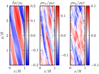
Figure 7: Pseudo-color images of the vertically integrated mass and momentum densities taken from the simulation described in Heinemann & Papaloizou (2009b).

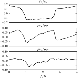
Figure 8: Cut through Figure 7 along $y$ at a fixed $x\approx 0.15$ (no average over $x$).

It should be noted that in an MRI simulation, spiral density waves propagate through a field of turbulent fluctuations, and it might be expected that the waves interact with these fluctuations. This could in general lead to wave front distortion and energy loses resulting from random secondary density wave generation through interaction of the primary wave with turbulent eddies (eg. Lighthill, 1953; Howe, 1971a, b; Ffowcs Williams & Howe, 1973). We also remark that a spiral density wave is expected to undergo wave front distortion as it propagates through a medium with local turbulent velocity and/or local sound speed fluctuations (eg. Hesselink & Sturtevant, 1988). This may occur in a stationary medium with no generation of secondary waves with different frequency.

We comment that a description of losses through wave-turbulence interactions by an effective turbulent viscosity is rather problematic. Such a description necessitates statistical averaging over many realizations of the system, see e.g. Balbus & Papaloizou (1999). Thus it most likely describes the possible variation that different realizations can display rather than the behavior of any one realization, where distortion of the wave profile rather than diffusion may occur, an issue that leads to interpretational difficulties, see Ffowcs Williams & Howe (1973) for an extensive discussion. These authors also point out that an effective turbulent viscosity description fails to meet the reasonable expectation that shock waves should be influenced mostly by small scale turbulent motions.

In support of the above view, we comment that experimental results presented by Plotkin & George (1972) for wave profiles associated with sonic booms propagating through a turbulent atmosphere indicate good agreement with non turbulent theory apart from random perturbations to the wave profile and a thickening of the shock front (that remains narrow on a macroscopic scale) (see also Giddings et al., 2001). Although the context differs, this view would appear to be consistent with the results presented in Figures 7 and 8.

Nonetheless, it is likely that interaction with disorganized turbulence causes the waves to decay more rapidly than predicted by our weakly nonlinear wave theory. An inspection of the results in Heinemann & Papaloizou (2009b) indeed indicates a decay rate faster than $t^{-2}$. However, this may be affected by the particular choices of Reynolds and Prandtl numbers that are made for numerical tractability. In this context it is important to note that the decay rate produced in the simple weakly nonlinear wave theory enunciated here gives, what we expect from the discussion above, to be a lower limit as far as the simulations are concerned and it does not differ greatly from what is actually observed. Thus the description of excited waves given by the simple theory and the current simulations is unlikely to be greatly modified when the transport coefficients are changed.

References

- Armitage (1998) Armitage P. J., 1998, ApJ, 501, L189+
- Balbus & Hawley (1991) Balbus S. A., Hawley J. F., 1991, ApJ, 376, 214
- Balbus & Hawley (1998) Balbus S. A., Hawley J. F., 1998, Reviews of Modern Physics, 70, 1
- Balbus & Papaloizou (1999) Balbus S. A., Papaloizou J. C. B., 1999, ApJ, 521, 650
- Ffowcs Williams & Howe (1973) Ffowcs Williams J. E., Howe M. S., 1973, Journal of Fluid Mechanics, 58, 461
- Fromang & Papaloizou (2007) Fromang S., Papaloizou J., 2007, A&A, 468, 1
- Gammie (1996) Gammie C. F., 1996, ApJ, 457, 355
- Gardiner & Stone (2005) Gardiner T. A., Stone J. M., 2005, in de Gouveia dal Pino, E. M. and Lugones, G. and Lazarian, A. ed., Magnetic Fields in the Universe: From Laboratory and Stars to Primordial Structures. Vol. 784 of American Institute of Physics Conference Series, Energetics in MRI driven Turbulence. pp 475–488
- Giddings et al. (2001) Giddings T. E., Rusak Z., Fish J., 2001, Journal of Fluid Mechanics, 429, 255
- Goldreich & Lynden-Bell (1965) Goldreich P., Lynden-Bell D., 1965, MNRAS, 130, 125
- Goodman & Rafikov (2001) Goodman J., Rafikov R. R., 2001, ApJ, 552, 793
- Hayes (1957) Hayes W. D., 1957, Journal of Fluid Mechanics, 2, 595
- Heinemann & Papaloizou (2009a) Heinemann T., Papaloizou J. C. B., 2009a, MNRAS, 397, 52
- Heinemann & Papaloizou (2009b) Heinemann T., Papaloizou J. C. B., 2009b, MNRAS, 397, 64
- Hesselink & Sturtevant (1988) Hesselink L., Sturtevant B., 1988, Journal of Fluid Mechanics, 196, 513
- Howe (1971a) Howe M. S., 1971a, Journal of Fluid Mechanics, 45, 785
- Howe (1971b) Howe M. S., 1971b, Journal of Fluid Mechanics, 45, 769
- Hunter & Keller (1983) Hunter J. K., Keller J. B., 1983, Communications on Pure and Applied Mathematics, 36, 547
- Landau & Lifshitz (1987) Landau L. D., Lifshitz E. M., 1987, Fluid Mechanics. Pergamon Press Ltd.
- Lighthill (1953) Lighthill M. J., 1953, in Proceedings of the Cambridge Philosophical Society Vol. 49 of Proceedings of the Cambridge Philosophical Society, On the energy scattered from the interaction of turbulence with sound or shock waves. p. 531
- Lin & Papaloizou (1996) Lin D. N. C., Papaloizou J. C. B., 1996, ARA&A, 34, 703
- Lynden-Bell & Ostriker (1967) Lynden-Bell D., Ostriker J. P., 1967, MNRAS, 136, 293
- Nelson (2005) Nelson R. P., 2005, A&A, 443, 1067
- Nelson & Papaloizou (2004) Nelson R. P., Papaloizou J. C. B., 2004, MNRAS, 350, 849
- Ogilvie & Lubow (1999) Ogilvie G. I., Lubow S. H., 1999, ApJ, 515, 767
- Papaloizou & Lin (1995) Papaloizou J. C. B., Lin D. N. C., 1995, ARA&A, 33, 505
- Parker (1992) Parker A., 1992, Proceedings: Mathematical and Physical Sciences, 438, 113
- Plotkin & George (1972) Plotkin K. J., George A. R., 1972, Journal of Fluid Mechanics, 54, 449
- von Neumann & Richtmyer (1950) von Neumann J., Richtmyer R. D., 1950, Journal of Applied Physics, 21, 232
- Yano (1996) Yano T., 1996, Shock Waves, 6, 313