Pattern formation in fast-growing sandpiles

Abstract

We study the patterns formed by adding $N$ sand-grains at a single site on an initial periodic background in the Abelian sandpile models, and relaxing the configuration. When the heights at all sites in the initial background are low enough, one gets patterns showing proportionate growth, with the diameter of the pattern formed growing as $N^{1/d}$ for large $N$, in $d$-dimensions. On the other hand, if sites with maximum stable height in the starting configuration form an infinite cluster, we get avalanches that do not stop. In this paper, we describe our unexpected finding of an interesting class of backgrounds in two dimensions, that show an intermediate behavior: For any $N$, the avalanches are finite, but the diameter of the pattern increases as $N^{\alpha}$, for large $N$, with $1/2<\alpha\leq 1$. Different values of $\alpha$ can be realized on different backgrounds, and the patterns still show proportionate growth. The non-compact nature of growth simplifies their analysis significantly. We characterize the asymptotic pattern exactly for one illustrative example with $\alpha=1$.

I Introduction

In the last two decades a large amount of study has been devoted to understanding various models of self-organized criticality, in particular, the Abelian Sandpile Model (ASM) (see dhar2006 ; redigleshouches for reviews). These have mainly dealt with the critical exponents of avalanches produced in sandpiles driven slowly in their critical steady state. But the ASM has other interesting properties, not directly related to its critical exponents. In particular, one sees very interesting and beautiful spatial patterns when many sand grains are added at a single point on an initially periodic background, and we relax the configuration using the ASM toppling rules. One such pattern on a square lattice is shown in Fig. 1.

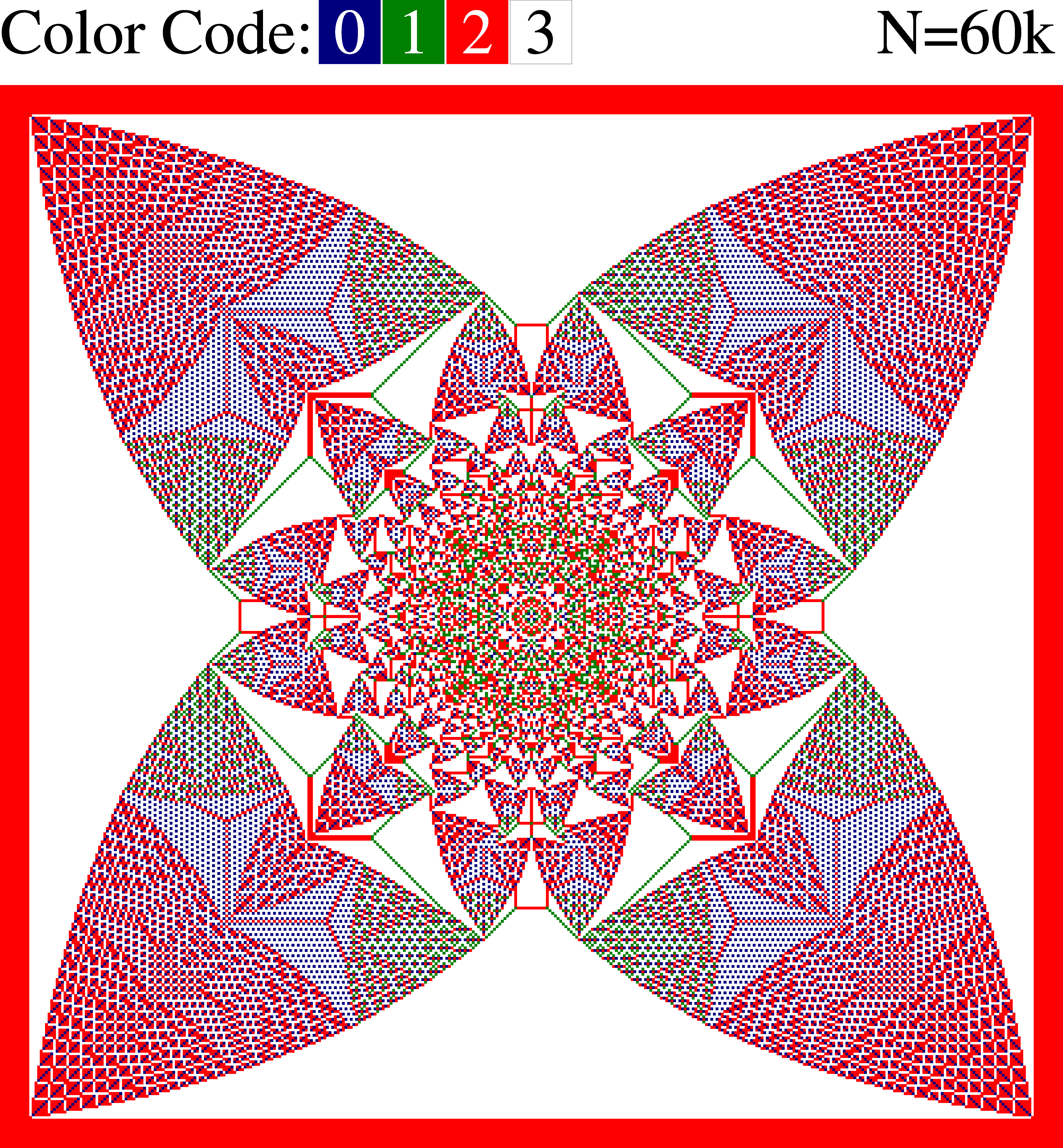
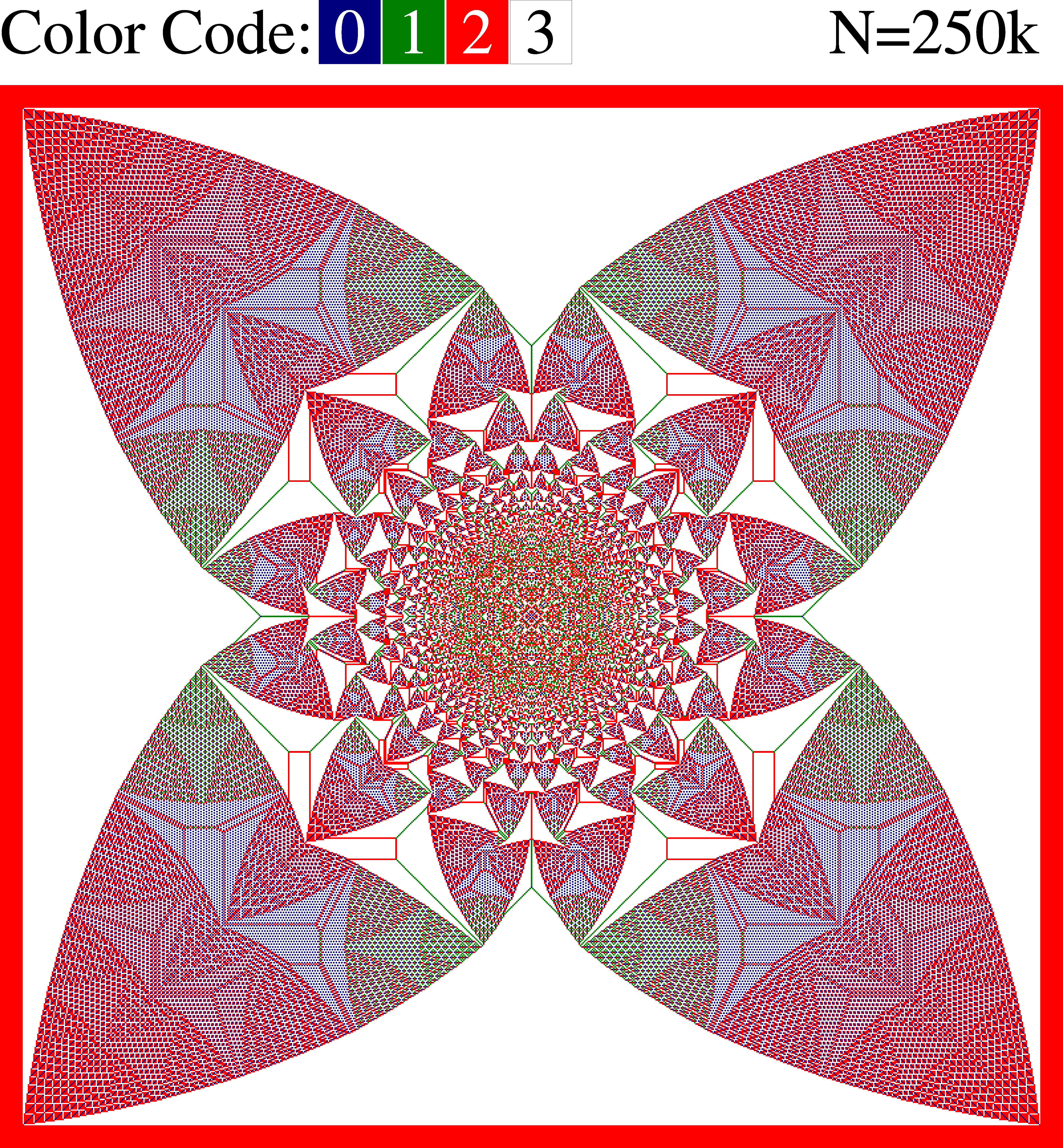
Figure 1: (Color online.) The stable configurations for the Abelian sandpile model on a square lattice, obtained by adding $N$ grains at the origin. In the initial configuration all heights are $2$. For comparison the size of the first figure has been enlarged by a factor $2$. (Details can be seen in the electronic version using zoom in).

Our interest in these patterns comes from several reasons. Firstly, these are analytically tractable examples of complex patterns that are obtained from simple deterministic evolution rules. Of course, there are many known examples of complex patterns obtained this way (e.g. Conway’s game of life earlierone ). But a detailed characterization of such patterns is usually not easy. The sandpile patterns studied here are special, as they are nontrivial, but of intermediate complexity, and are analytically tractable.

Secondly, growing sandpiles studied here are qualitatively different from the growth models that have been studied in physics literature earlier, such as the Eden model, the diffusion limited aggregation, or the surface deposition eden ; dla ; barabasi . These are the simplest models of proportionate growth, a well-known feature of biological growth in animals, where different parts of a growing animal grow at roughly the same rate, keeping their shape almost the same. In the models of growth studied earlier, growth is confined to some active outer region. The inner structures, once formed are frozen, and do not evolve further in time. This is not the case for the patterns studied in this paper. Figure 1 shows two patterns produced on the same background but with different values of the number $N$ of grains added. As $N$ increases, the pattern grows in size, but we see that while some new details emerge near the center, the relative proportions of different parts in the outer region of the pattern remains unchanged. As the pattern grows, different features, not only grow in size, but also are moved in space with time.

The third motivation for our study is some intriguing connection of these to the mathematics of discrete analytic functions. We have not explored this much, but will discuss briefly in an appendix.

There have been several earlier studies of the spatial patterns in sandpile models. First of them was by Liu et.al. liu . The asymptotic shape of the boundaries of the patterns produced in centrally seeded sandpile model on different periodic backgrounds was discussed in dhar99 . Borgne et.al. borgne obtained bounds on the rate of growth of these boundaries, and later these bounds were improved by Fey et.al. redig and Levine et.al. lionel2 . A detailed analysis of different periodic structures found in the patterns were first carried out by Ostojic ostojic who also first noted the exact quadratic nature of the toppling function within a patch. Wilson et.al. wilson have developed a very efficient algorithm to generate patterns for a large numbers of particles added, which allows them to generate pictures of patterns with $N$ up to $2^{26}$.

Other special configurations in the Abelian sandpile models, like the identity borgne ; identity ; caracciolo or the stable state produced from special unstable states, also show complex internal self-similar structures liu , which share common features with the patterns studied here. In particular, the identity configuration on the F-lattice has recently been shown to have similar spatial structures caracciolo .

There are other models, which are related to the Abelian sandpile model, e.g., the Internal Diffusion-Limited Aggregation (IDLA) lawler , Eulerian walkers (also called the rotor-router model) abhishek ; lionel1 ; propprotor , and the infinitely-divisible sandpile lionel2 , which also show similar structure. For the IDLA, Gravner and Quastel showed that the asymptotic shape of the growth pattern is related to the classical Stefan problem in hydrodynamics, and determined the exact radius of the pattern with a single point source gravner . Levine and Peres have studied patterns with multiple sources in these models, and proved the existence of a limit shapelionel3 . Limiting shapes for the non-Abelian sandpile has recently been studied by Fey. et.al. nonab .

The standard square lattice produces complicated patterns and it has not been possible to characterize them fully, so far. In an earlier paper myepl , we considered the pattern produced on a F-lattice (Fig. 2(a)), and determined exactly the sizes of different patches in the asymptotic pattern. The pattern produced by adding grains at one site on a background with a periodic chequerboard pattern of alternate sites with heights $1$ and $0$, is shown in the Fig. 2(b). In paper myjsp , we studied the patterns when sink sites are present, or when addition is made at more than one site. In paper myjsm , we have studied the effect of noise on such patterns.

If the average initial height in a background is high, one gets infinite avalanches, with the diameter of the pattern becoming infinite for finite number of particles added. Such backgrounds have been termed as ‘explosive’. In other cases, the diameter of the pattern is finite for any finite $N$, and increases as $N^{1/d}$ in $d$-dimensions. We call such a growth as compact growth. All the patterns studied in myepl ; myjsp ; myjsm showed compact proportionate growth. In this paper, we describe a remarkable class of patterns where the diameter remains finite for any finite $N$, but grows as $N^{\alpha}$, with $1/2<\alpha\leq 1$. We call such growth as non-compact proportionate growth. Characterization of these patterns, as will be shown, is simpler than in the compact case.

We found two classes of backgrounds, both infinite, on a directed triangular lattice (see Fig. 4), for which the growth is proportionate, with the growth exponent $\alpha=1$. Our numerical study shows, but we have no formal proof, that different backgrounds belonging to the same class produce the same asymptotic pattern. In addition, we found infinitely many backgrounds on the F-lattice which produce patterns with proportionate non-compact growth. However, in these cases the growth exponent $\alpha$ takes a different value, with $1/2<\alpha<1$ for each member.

There are some earlier works on the growth rate of the sandpile patterns. Different non-explosive backgrounds for a DASM were studied in redig ; lionel2 ; explosion . However, in all these examples, studied so far, the growth of the patterns is compact. For a DASM on a square lattice, it was shown explosion , that the pattern produced on a background of constant height $z\leq z_{c}-2$, is always enclosed inside a square whose width grows as $\sqrt{N}$.

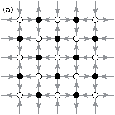
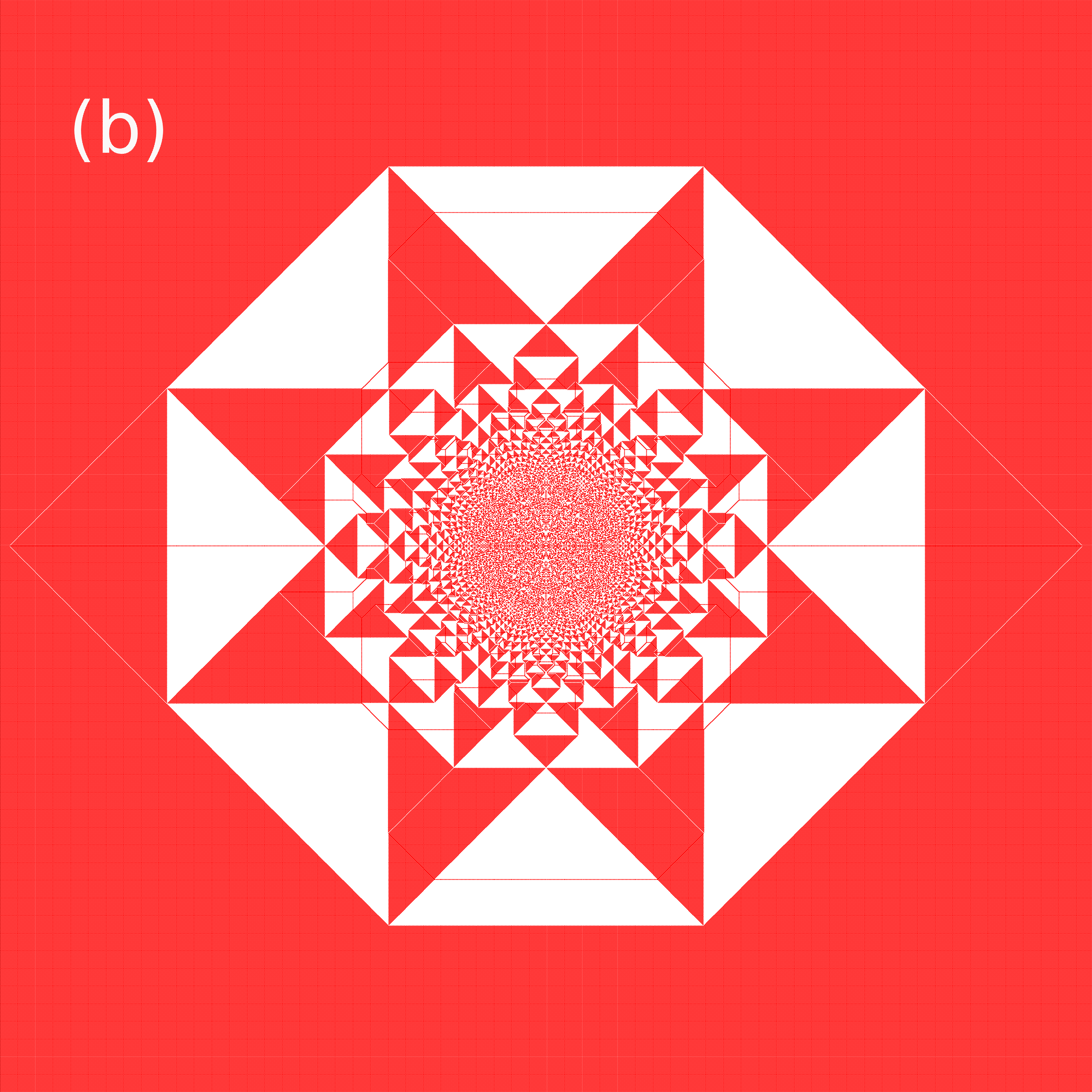
Figure 2: (Color online.) (a) A F-lattice with directed bonds, and a chequerboard distribution of grains on it. Unfilled circles denote height $z=1$ and filled ones $z=0$. (b) The stable configuration obtained by adding $10^{5}$ grains at the origin. Color code: red =0, white = 1. The apparent orange regions in the picture represent the patches with checkerboard configuration. (Details can be seen in the electronic version using zoom in.)

We also discuss the exact characterization of the pattern shown in Fig. 11, one of the two asymptotic patterns we have found with $\alpha=1$. This is described, as in the earlier studied case of compact growth myepl , in terms of the scaled toppling function. However, the analysis of non-compact patterns is actually simpler. Clearly, for $\alpha>1/d$, the mean excess density of particles in the toppled region is zero, for the asymptotic non-compact growth patterns. The patterns are made of large regions where the heights are periodic, and we call them as patches. We find that, inside each patch, the mean density is exactly the same as in the background, and the excess grains are concentrated along the patch boundaries. There are also some boundaries where excess grains density is negative. We show that this leads to the scaled toppling function being a piece-wise linear function of the rescaled coordinates. Thus, in each patch, the potential function is specified by only $3$ coefficients. In contrast, for the compact patterns, the scaled toppling function is a quadratic function of the coordinates in each patch myepl , and one has to determine $6$ coefficients for each patch, to determine the function fully.

We are able to reduce the problem of determining the asymptotic pattern in Fig. 11 to that of finding the lattice Green’s function on a hexagonal lattice. This is known to be expressible as integrals that can be evaluated in closed form atkinson , and this leads to a full solution of the problem. For the compact growth patterns studied earlier on F-lattice myepl ; myjsp , we define a discrete analytic function $F_{p}(z)$, which is the discrete analogue of the analytic function $z^{p}$, for any rational value of $p$, and show that the patterns can be characterized in terms of this function.

The plan of this paper is as follows: In section II, we discuss how different periodic background configurations give rise to different rates of growth. In section III, we describe two classes of periodic background configurations on a directed triangular lattice that give rise to patterns which show proportionate growth with $\alpha=1$. In section IV we argue that, for any pattern with non-compact proportionate growth the rescaled toppling function is piece-wise linear. In section V, we discuss exact characterization of the simplest of the patterns with $\alpha=1$. Patterns on the F-lattice, with $1/2<\alpha\leq 1$ are discussed in section VI. Section VII contains some concluding remarks and a discussion about connection to tropical polynomials. An appendix describes how the characterization of these patterns involves the theory of discrete analytic functions defined on many-sheeted discretized Riemann surfaces.

II The compact and non-compact growth patterns

The simplest growing patterns are found in the Manna-type sandpile models with stochastic toppling rules sasm . In these models, when the density of particles $\rho_{o}$ in the background is small, the avalanches are always finite. In the relaxed configuration, the toppled sites form a nearly circular region (see Fig. 3). The asymptotic pattern seems to be perfectly circular disc of uniform density, with an average density $\rho^{\star}$ inside the circle and $\rho_{o}$ outside. The value of $\rho^{\star}$ is independent of the background density $\rho_{o}$, and is equal to the unique steady state density of the corresponding self organized critical model with random sites of addition, and dissipation at the boundary sasm . The region inside the circle forgets about the initial height configuration, and is in the self-organized critical state. The boundary of the affected region is thin with a sharp transition of density from $\rho^{\star}$ to $\rho_{o}$. Then considering that, for large $N$, all the added grains are confined inside the circular region of diameter $2\Lambda$, we get

$$N=\left(\rho^{\star}-\rho_{o}\right)\pi\Lambda^{2}+\rm{Lower~{}order~{}in~{}}\Lambda.$$ (1)

Thus the pattern has a compact growth.

For densities $\rho_{o}$ close to, but below $\rho^{\star}$, sometimes a single particle addition can lead to very large increase in the size of the toppled region. However, probability of such large jumps decreases exponentially with size, and for any finite $N$, with probability $1$, avalanches remain finite. As long as $\rho_{o}$ is less than $\rho^{\star}$, the system relaxes, forming a pattern whose diameter grows as $\sqrt{N}$. Adding a single grain on a background of super-critical density ($\rho>\rho^{\star}$) gives rise to infinite avalanches, with non-zero probability. Then, with probability $1$, such backgrounds will lead to an infinite avalanche for some finite value of $N$. In higher dimensions also, a similar behavior is expected.

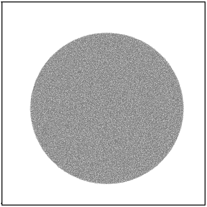
Figure 3: The pattern produced by adding $N=10^{5}$ grains at a single site on a stochastic ASM defined on an infinite square lattice, and relaxing the configuration. The initial configuration has all sites empty. The threshold height $z_{c}=2$, and on toppling two grains are transfered either to the vertical or horizontal neighbors, with equal probability. Color code: White=0, and Black=1.

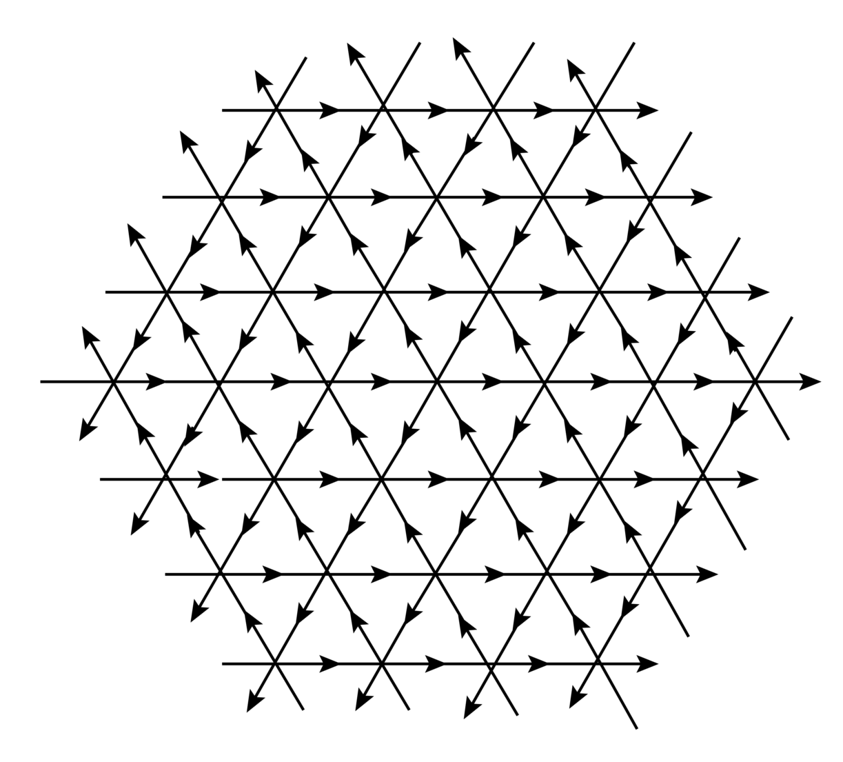
Figure 4: A directed triangular lattice.

In the models with deterministic relaxation rules there is no simple quantifier like critical density $\rho^{\star}$, separating the explosive and non-explosive backgrounds. Whether the periodic or random background is explosive or not depends in a complicated way on the built-in height correlations. For example consider the BTW model on a square lattice, where the steady state density $\rho^{\star}=17/8=2.125$ sasm . It has been shown that a background with a random assignment of height $3$ with probability $\epsilon$, on a sea of constant height $2$ is explosive, even for arbitrary small value of $\epsilon$ explosion , although the average density $\rho_{o}=2+\epsilon$ is much less than $\rho^{\star}$. On the other hand, it is also possible to construct a robust periodic background with density arbitrarily close to maximum stable height $3$ explosion .

We will show that there is a large class of backgrounds, with a range of densities, for which the growth is less than explosive, but more than compact.

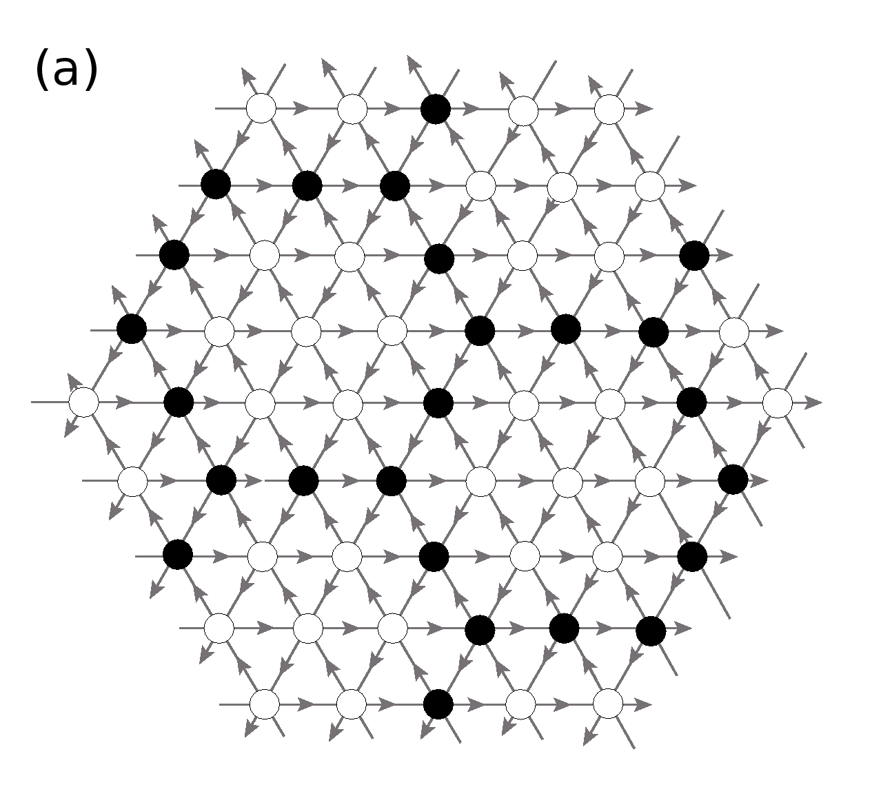
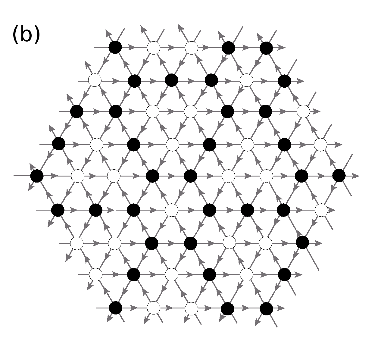
Figure 5: Examples of backgrounds of class I and II, respectively. The filled circles represent height $1$ and unfilled ones height $2$.

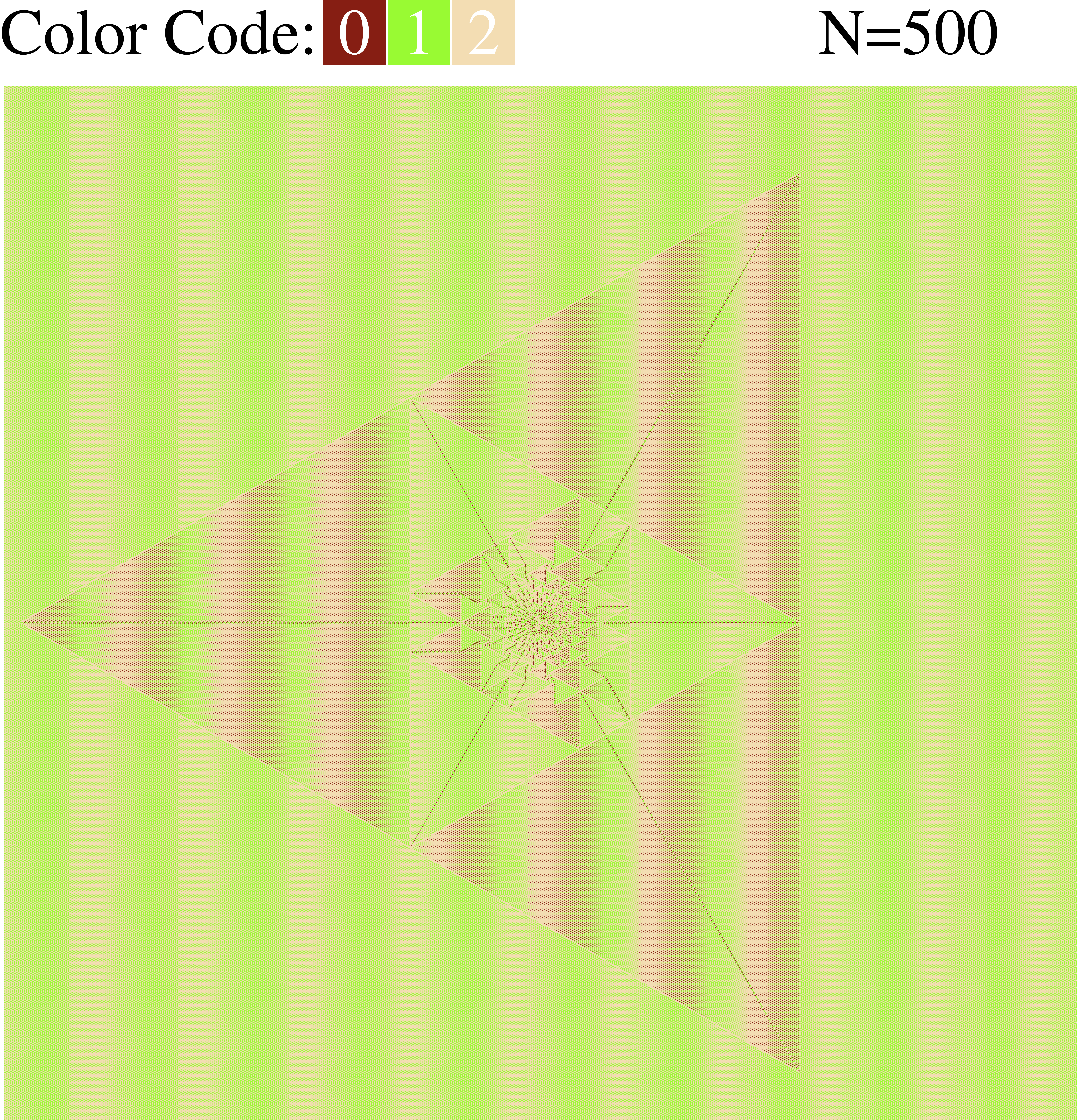
Figure 6: (Color online.) The class I pattern, formed by adding $N=500$ particles at the origin on the first background shown in Fig. 5. The apparent uniform green color of the background is actually a periodic structure. Details can be viewed in the electronic version using zoom in.

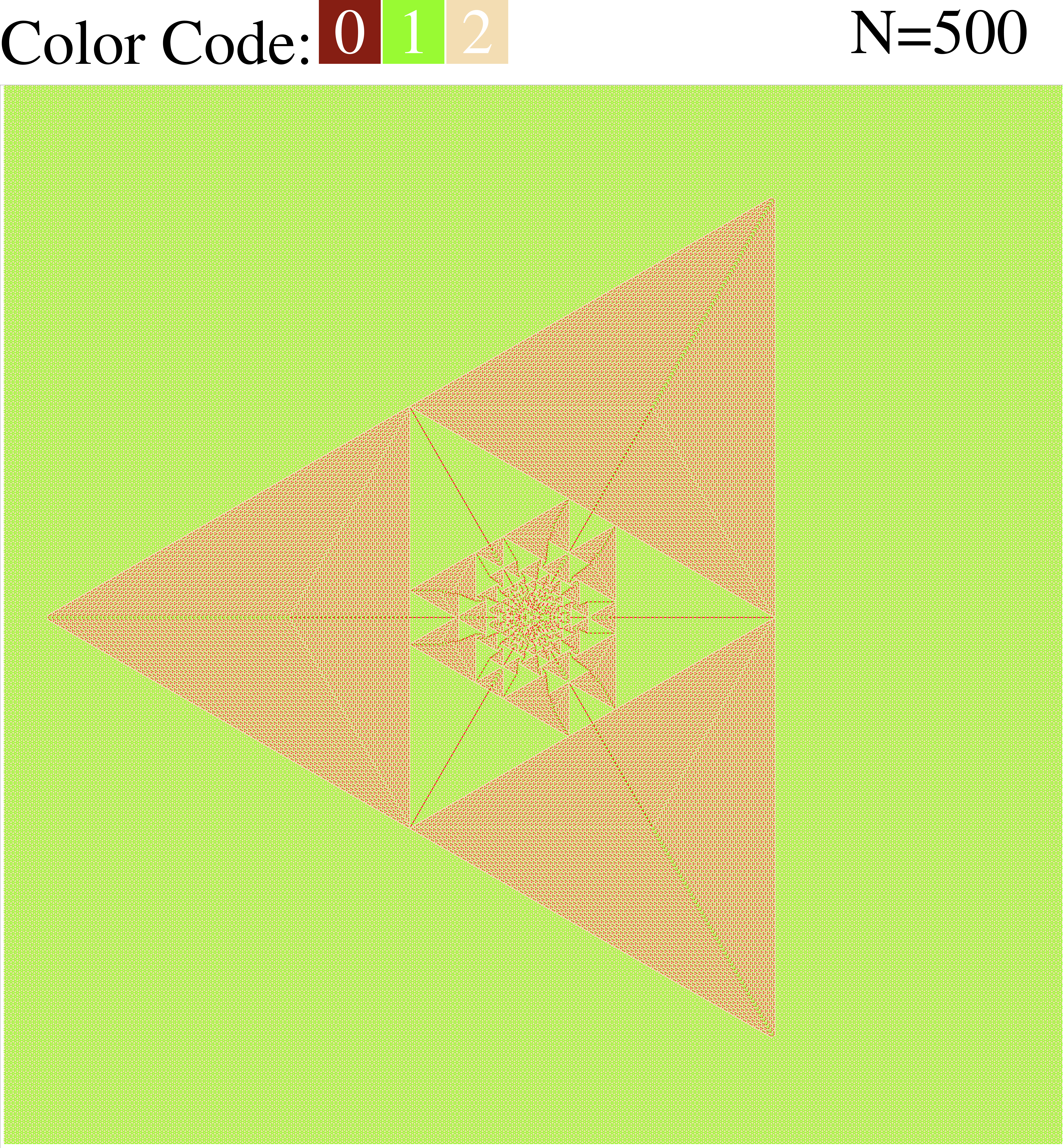
Figure 7: (Color online.) The class II pattern, formed by adding $N=500$ particles at the origin on the second background in Fig. 5. The apparent uniform green color of background is actually a periodic structure. Details can be viewed in the electronic version using zoom in.

III Examples of non-compact growth

We first discuss the patterns with $\alpha=1$. We start with a ASM on a directed graph corresponding to an infinite two dimensional triangular lattice, with each site having three incoming and three outgoing arrows (see Fig. 4). The threshold height $z_{c}=3$, for each site. If the height at any site is above or equal to $z_{c}$, it is unstable, and relaxes by toppling: in each toppling, three sand grains leave the unstable site, and are transferred one each along the directed bonds going out of the site.

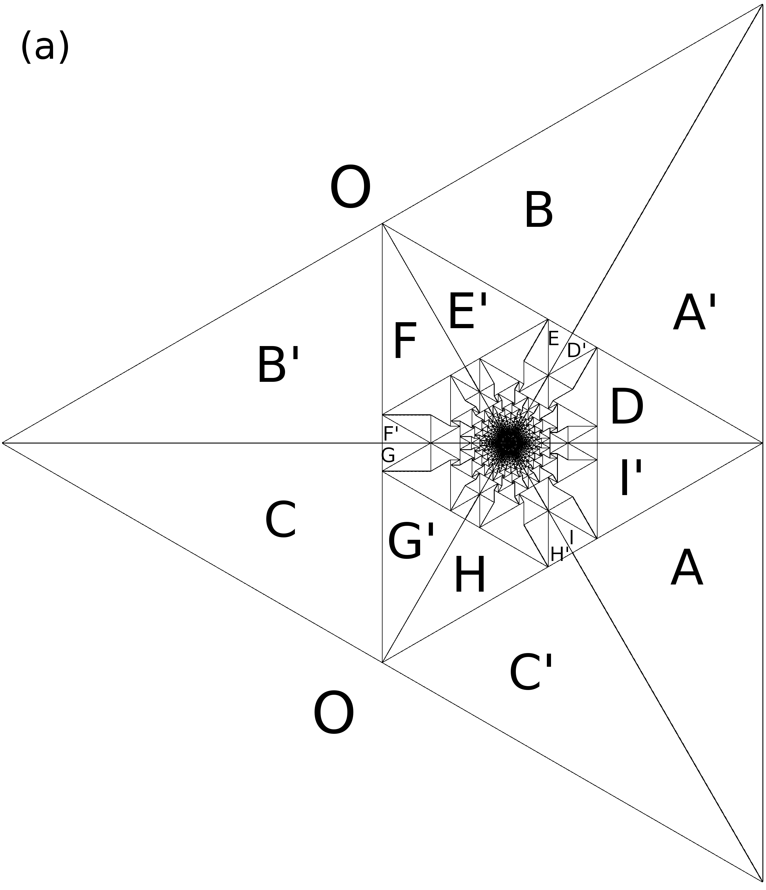
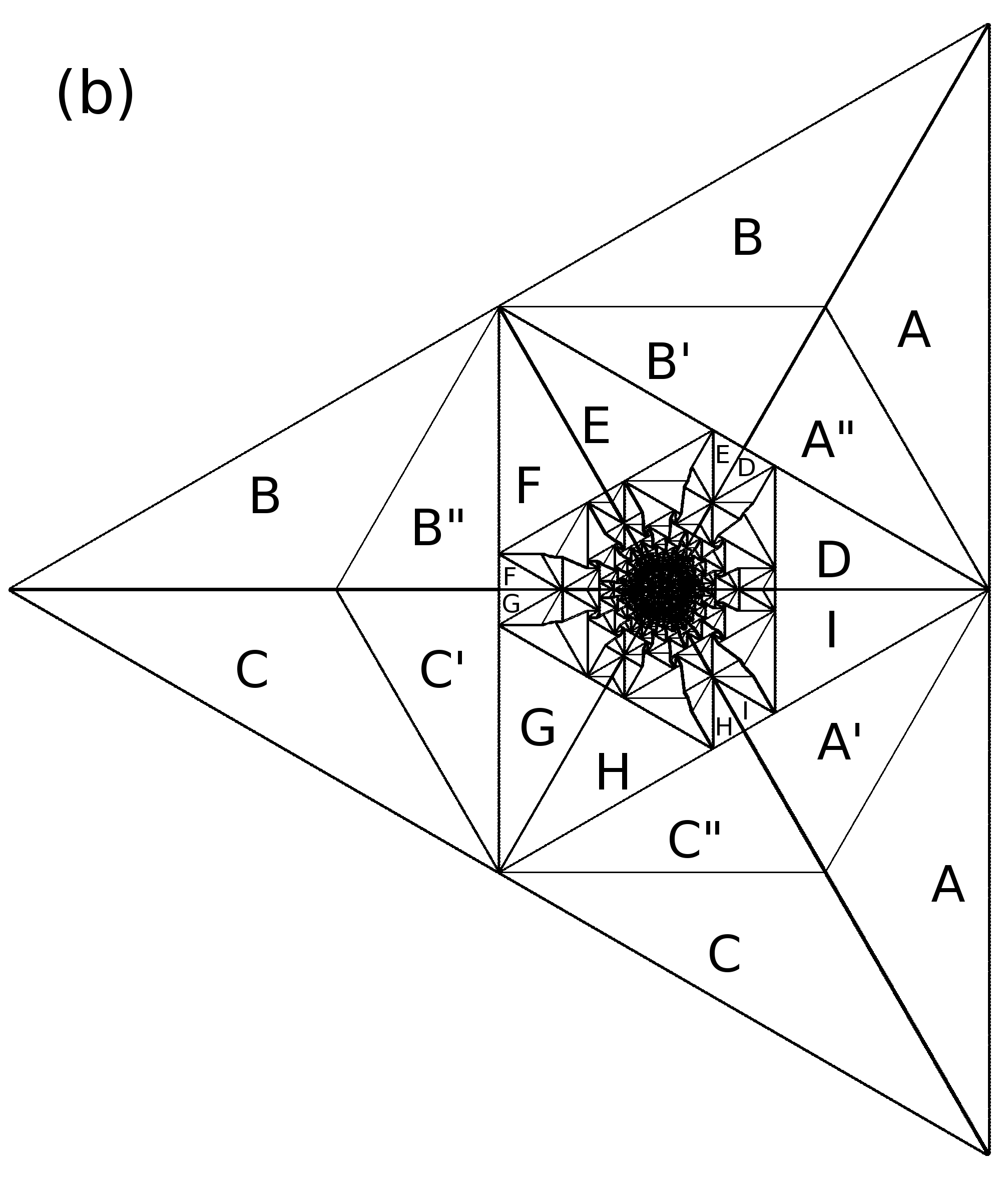
Figure 8: The patterns in terms of $Q\left(r\right)$, corresponding to those in Fig. 6 and 7. Sites with zero $Q\left(r\right)$ are colored white, and non-zero are colored black. The larger patches are given identifying labels.

We consider two classes of backgrounds on this lattice:

• Class I: We consider the lattice as made of triangular plaquettes, which are joined together to make tiles in the shape of regular hexagons with edges of length $l$. We cover the two-dimensional plane with these tiles. Sites that lie on the boundaries of these hexagons are assigned height $1$, and the rest of the sites have height $2$. Figure 5$(a)$ shows the background configuration for the case $l=2$.

• Class II: For these backgrounds, we cover the two-dimensional plane with tiles in the shape of equilateral triangles of edge-length $l$. The sites that lie on the boundaries of the triangles, and are shared by two triangles, are assigned height $1$, and remaining sites are assigned height $2$. Sites that are at the corners of triangular tiles, and shared by six of them, are also assigned heights $2$. The background configuration corresponding to $l=4$ is shown in figure 5$(b)$. The pattern made of triangular tiles with $l=3$ is same as the class I background with hexagon of edge-length $1$. Hence, only patterns formed with triangles of edge-length $l\geq 4$ will be said to be in this class.

The patterns produced by adding $N$ grains, where $N$ is large, at a single site on the two backgrounds in Fig. 5 are shown in Fig. 6 and 7. While the patterns look quite similar, a closer examination shows that they are not identical. In Fig. 7, there are extra lines of particles within the brownish patches which break each patch into smaller parts. In fact, with the identification of some patches having only a point in common, as discussed later, we can show that each patch breaks into exactly three patches. These three parts have similar periodic pattern, but with different orientations.

This differences can be seen more clearly in terms of the net excess change in height ${Q\left(R\right)}$ in a unit cell centered at $R$, where the unit cell is that of the background pattern.

$$Q\left(R\right)=\sum_{R^{\prime}\in\textrm{unit cell}}\Delta z(R+R^{\prime}),$$ (2)

where $\Delta z\left(R\right)$ is the change in height at site $R$. For example in the first background in Fig. 5 a unit cell is a hexagon of edge length $l=2$, and for the second background it is a parallelogram of each side length $l=4$. A site that is on the edge of the unit cell is counted with weight $1/2$, and a site on the corner of the hexagon with weight $1/3$, and on the corner of the parallelogram with weight $1/4$. By construction, the function $Q\left(r\right)$ is zero inside each patch, and non-zero along the boundaries between patches. The patterns in terms of these variables, corresponding to those in Fig. 6 and 7 are shown in Fig. 8.

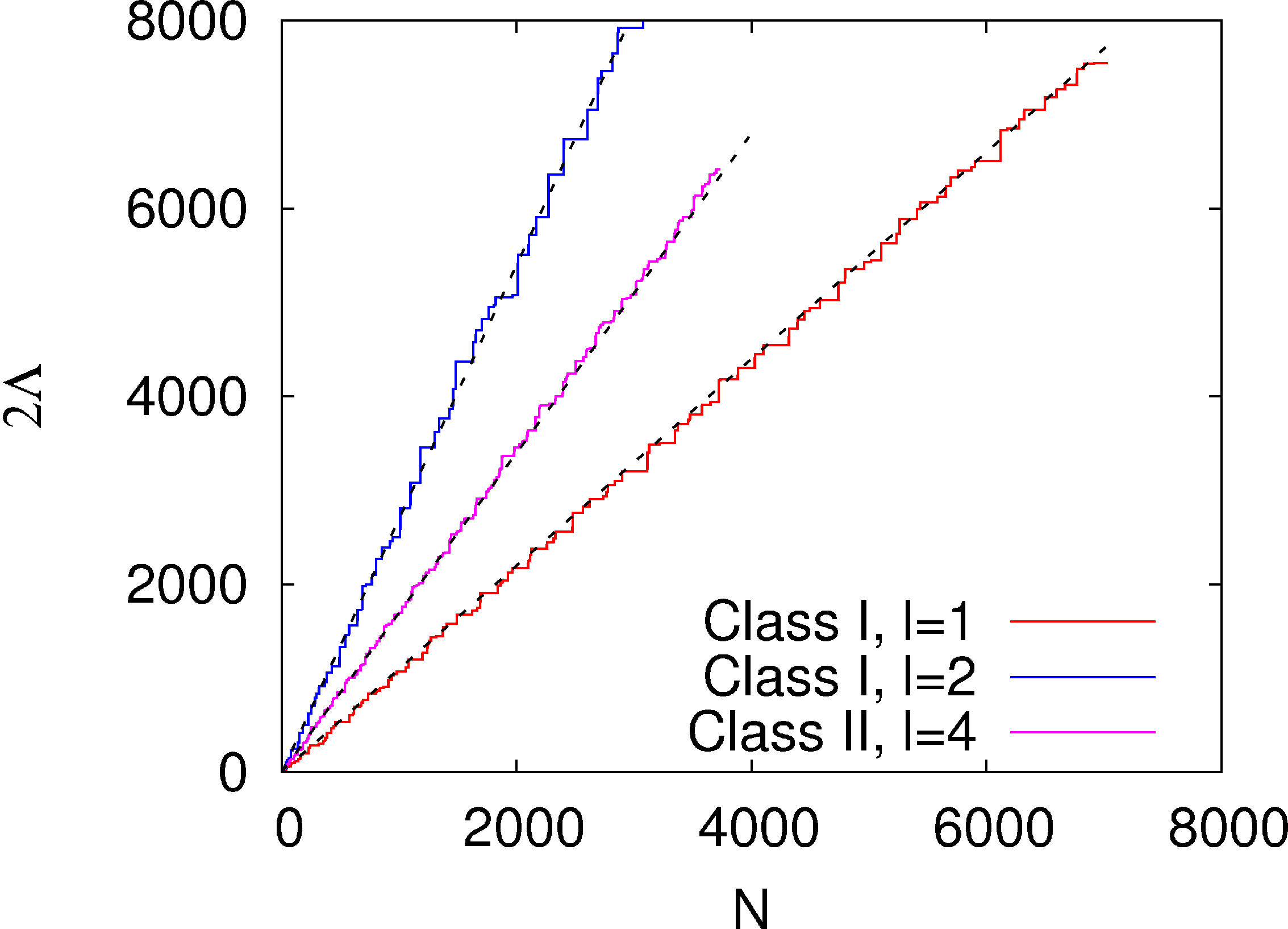
Figure 9: (Color online.) The diameter $2\Lambda$ of the patterns as a function of the number $N$ of added grains. The cases shown are (i) Class I, $l=1$, (ii) Class I, $l=2$, and (iii) Class II , $l=4$. The corresponding straight line fits have slopes given by $1.1$, $2.7$ and $1.7$ respectively.

We have seen that the patterns on these two classes of backgrounds exhibit proportionate growth, i.e., all the spatial features inside the patterns for large $N$, grow at the same rate with the diameter. We define the diameter $2\Lambda$, in general, for any pattern in this paper, as the height of the smallest rectangle containing it. For the patterns in Fig. 6 and Fig. 7, it is then the length of a side of the bounding equilateral triangle. This particular choice makes $2\Lambda$ as an integer multiple of $\sqrt{3}$, on the triangular lattice. We find that for both types of backgrounds in Fig. 5, the diameter of the pattern grows linearly with $N$ (Fig. 9).

IV Piece-wise linearity of the toppling function.

Considering the proportionate growth, let us define a rescaled coordinate $\vec{r}=\vec{R}/N^{\alpha}$, where $\vec{R}\equiv\left(x,y\right)$ is the position vector of a site on the lattice. The number of topplings at any site inside the pattern, scales linearly with $N$. Let us define

$$\phi\left(\vec{r}\right)=\lim_{N\rightarrow\infty}\frac{T_{N}(\vec{R})}{N}.$$ (3)

We now show, using an extension of the argument given in myepl , that the function $\phi$ is linear inside periodic patches in all the patterns with non-compact growth, i.e., with $\alpha>1/2$. Within a patch, the function $\phi(\vec{r})$ is expandable in Taylor series around any point $\vec{r}_{o}$, not on the boundary of the patch. Defining $\vec{r}_{o}\equiv\left(\xi_{o},\eta_{o}\right)$, and $\Delta\vec{r}_{o}\equiv\left(\Delta\xi,\Delta\eta\right)$ we have

$$\phi\left(\xi_{o}+\right. \Delta\xi,\left.\eta_{o}+\Delta\eta\right)-\phi\left(\xi_{o},\eta_{o}\right)$$ (4)

$$=d\Delta\xi+e\Delta\eta+\mathcal{O}\left(\Delta\xi^{2},\Delta\eta^{2},\Delta\xi\Delta\eta\right).$$

Consider any term of order $\geq 2$ in the expansion, for example, the term $\sim(\Delta\xi)^{2}$. This can only arise due to a term $\sim(\Delta x)^{2}N^{1-2\alpha}$ in the toppling function $T_{N}(\vec{R})$. Then, considering the fact that $T_{N}(\vec{R})$ is an integer function of $x$ and $y$, it is easy to see that this term would lead to discontinuous changes in $T_{N}(\vec{R})$ at intervals of $\Delta x\sim\mathcal{O}(N^{\alpha-1/2})$. As $\alpha>1/2$ for non-compact growth patterns, this leads to a change in the periodicity of heights at such intervals inside each patch which themselves are of size $\sim N^{\alpha}$. This would then result in many defect lines within a patch, in the pattern at large $N$. However there are no such features in Fig. 11. Therefore inside each periodic patch, $\phi(\vec{r})$ must be exactly linear in $\vec{r}$. In fact, it turns out that the integer toppling function $T_{N}(\vec{R})$ is exactly linear inside a patch even for any finite $N$, except for an additional periodic term of periodicity equal to that of the heights inside the patch.

Another consequence of the exact linearity of the potential function in each patch is that all patch boundaries in the asymptotic pattern are straight lines.

The argument finally relies on the two observed (not rigorously established) features of the patterns, i.e., there is proportionate growth, and that the patterns can be decomposed in terms of periodic patches which are themselves of size $\mathcal{O}\left(N^{\alpha}\right)$.

Let us write the toppling function $T_{N}(\vec{R})$ within a single patch $P$ as

$$T_{N}(\vec{R})=A_{P}+\vec{K}_{P}\cdot\vec{R}+T_{periodic}(\vec{R}),$$ (5)

where $T_{periodic}(\vec{R})$ is a periodic function of its argument with zero mean value. If $\hat{e}_{1}$ and $\hat{e}_{2}$ are the basis vectors at the unit cell of the periodic pattern then we have

$$T_{N}(\vec{R}+\hat{e}_{1})-T_{N}(\vec{R}) = \vec{K}_{P}\cdot\hat{e}_{1},$$

$$T_{N}(\vec{R}+\hat{e}_{2})-T_{N}(\vec{R}) = \vec{K}_{P}\cdot\hat{e}_{2}.$$ (6)

As $T_{N}(\vec{R})$ are integer valued functions, $\vec{K}_{P}\cdot\hat{e}_{1}$ and $\vec{K}_{P}\cdot\hat{e}_{2}$ can only take integer values. If $\hat{g}_{1}$ and $\hat{g}_{2}$ are the unit vectors in the reciprocal space of the super lattice of the periodic pattern,

$$\hat{g}_{i}\cdot\hat{e}_{j}=\delta_{ij}\textrm{~{} ~{} ~{} ~{} }i,j=1,2,$$ (7)

then $\vec{K}_{P}$ must be an integer linear combination of $\hat{g}_{1}$ and $\hat{g}_{2}$, and can be written as

$$\vec{K}_{P}=n_{1}\hat{g}_{1}+n_{2}\hat{g}_{2},$$ (8)

where $n_{1}$ and $n_{2}$ are some integers. For example, in the background pattern in Fig. 10, a choice of the basis vectors and its reciprocal vectors is

$$\hat{e}_{1}\equiv\left(\frac{3}{2},\frac{\sqrt{3}}{2}\right); \mathrm{~{}~{}~{}~{}~{}}\hat{e}_{2}\equiv\left(\frac{3}{2},-\frac{\sqrt{3}}{2}\right)$$

$$\hat{g}_{1}\equiv\frac{2}{3}\left(-\frac{1}{2},-\frac{\sqrt{3}}{2}\right); \mathrm{~{}~{}~{}~{}~{}}\hat{g}_{2}\equiv\frac{2}{3}\left(-\frac{1}{2},\frac{\sqrt{3}}{2}\right).$$ (9)

The fact that $K_{{}_{P}}$ is constant inside a patch, implies that the patches can be labeled by the pair of integers $\left(n_{1},n_{2}\right)$.

An interesting consequence of this linear dependence of $T_{N}(\vec{R})$ is that there are no transient structures within the patches. On increasing $N$, if the $A_{{}_{P}}$ function increases, all sites in the patch $P$, except possibly those at the patch boundaries, undergo same number of additional topplings.

V Characterizing the class I asymptotic patterns

We now discuss characterization of the asymptotic pattern of class I, showing $\alpha=1$. In this section we quantitatively characterize the asymptotic pattern for the case $l=1$. The background configuration is shown in Fig. 10. A site on the triangular lattice can be labeled uniquely by a pair of integers $\left(p,q\right)$, such that its position on a complex plane can be written as $\mathbf{R}=p+q\omega$, where $\omega=\exp\left(i2\pi/3\right)$ is a complex cube root of unity. Then, the height variables in the background pattern in Fig. 10, can be written as

$$h(p+q\omega) = 2\textrm{ if }p+q=0\textrm{ (mod 3),}$$ (10)

$$= 1\rm{~{}~{}~{}otherwise.}$$

The average height in the background, $\langle z\rangle=4/3$. The configuration of the pile produced on this background, by adding $N=3760$ grains at the origin is shown in Fig. 11.

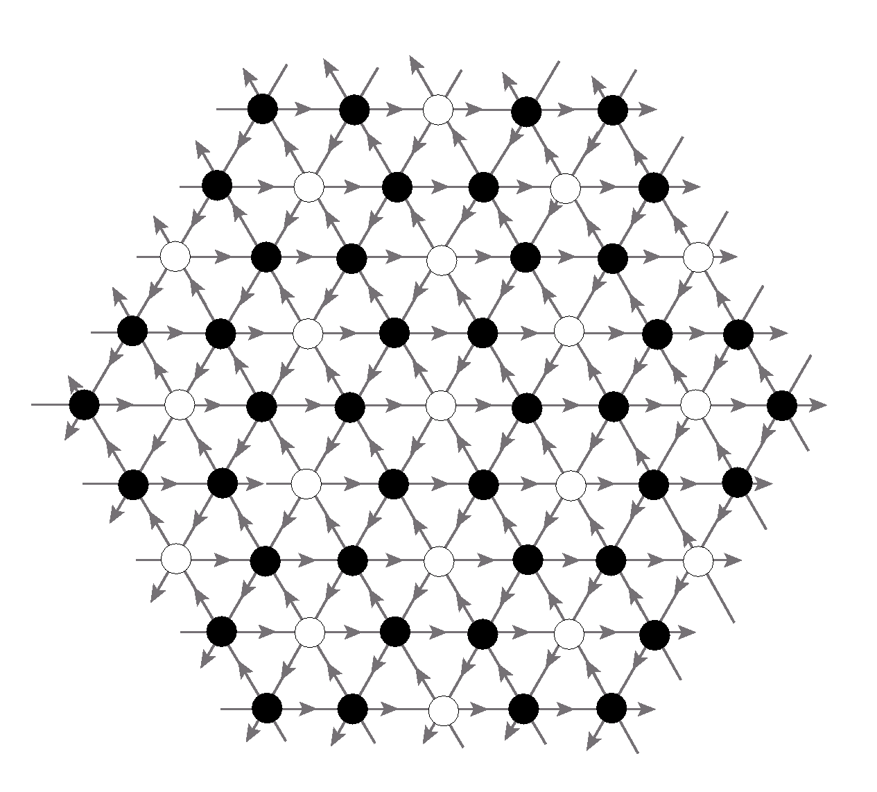
Figure 10: The background of class I corresponding to $l=1$. The filled circles represent height $z=1$ and unfilled ones $z=2$.

Figure 11: (Color online.) The pattern produced by adding $N=3760$ grains at a single site on the background in Fig. 10, and relaxing. Details can be seen in the online version using zoom-in

We see that the sites toppled due to addition of the grains are confined within an equilateral triangle. The pattern can be thought of as a union of patches, inside which the heights are periodic. A zoom-in showing the height configuration with five patches meeting at a point is shown in Fig. 12. There are only two types of periodic patches seen: one is like the background, where the sites of height $2$ are surrounded by sites of height $1$, and the other with heights $0$ surrounded by heights $2$. Then, the average height $\langle z\rangle$ inside both types of patches are same. In fact, it is equal to that of the background, $\langle z\rangle=4/3$.

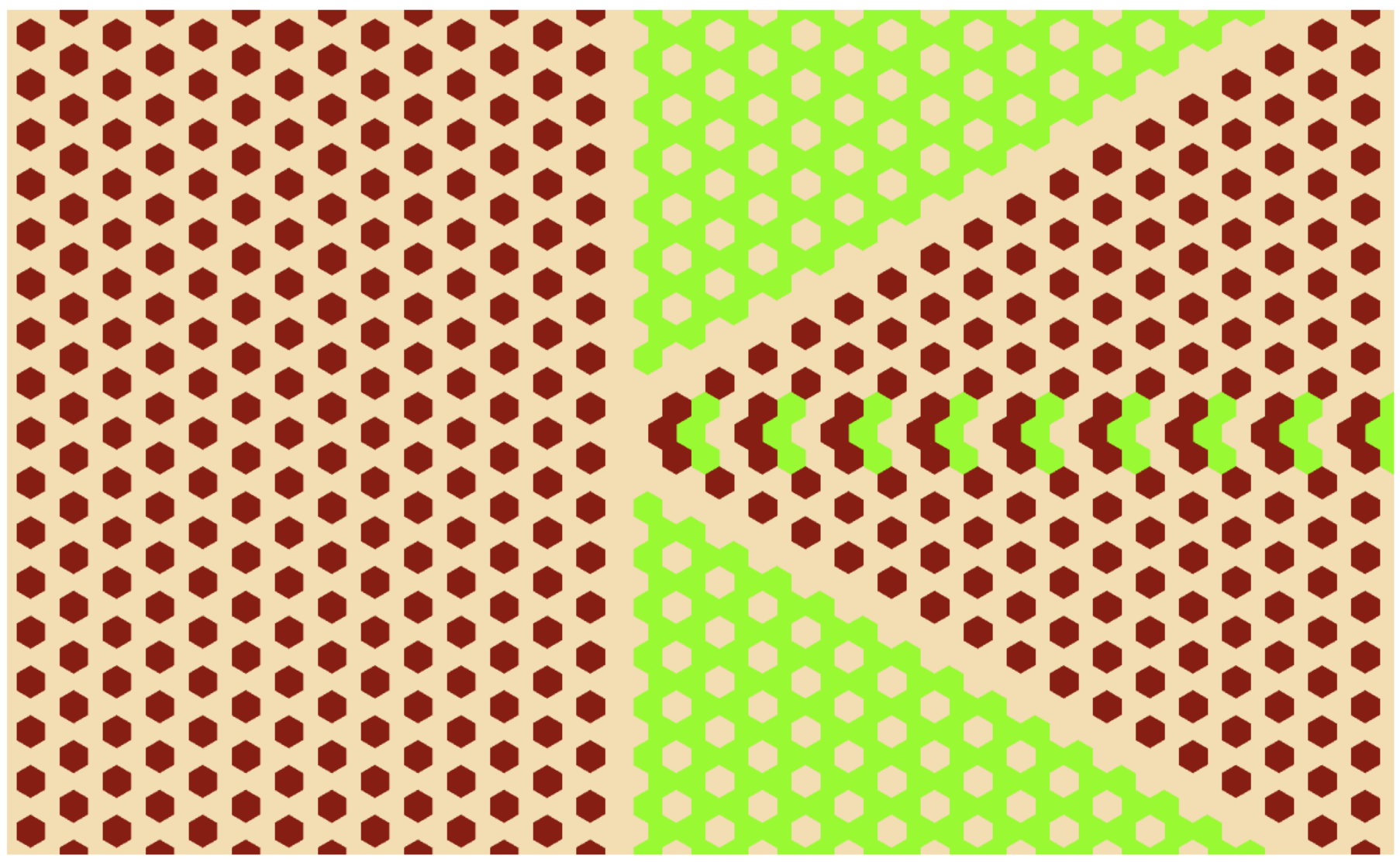
Figure 12: (Color online.) An example of patch boundaries in Fig. 11 meeting each other. Each filled hexagon represents Wigner cell around a site, and the color in them denotes height of that site. The color code is same as in Fig. 11.

The patches in the outer region of the pattern are big, and they become smaller, and more numerous as we go inwards. Along the common boundary of adjacent patches, we see line-like defect structures, and only along these lines the density is different from the background. In Fig. 12, one can also see the periodicity of the structures along the patch boundaries. Some patch boundaries, like the horizontal boundary in Fig. 12, have a deficit of particles compared to the background.

The boundaries of the patches are seen more clearly in terms of $Q(\mathbf{R})$ variables, as shown in figure 8(a), where we have labelled different patches as $\mathbf{A,A^{\prime},B,B^{\prime}}...$ etc..

The dependence of $2\Lambda$ on $N$ for this background is shown in Fig. 9. We see that the diameter for the pattern grows asymptotically linearly with $N$, but it grows in bursts: it remains constant for a long interval as more and more grains are added, and suddenly increases by a large amount at certain values of $N$. For example, at $N=3721$, the $2\Lambda$ is $2276\sqrt{3}$, and it jumps to a value $2408\sqrt{3}$ when one more grain is added. Let $J_{max}(N_{m})$ denote the size of the maximum jump in $2\Lambda$ encountered, as $N$ is varied from $1$ to $N_{m}$. In Fig. 13, we have plotted the variation of $J_{max}(N_{m})$ with $N_{m}$. The graph is consistent with a power-law growth, with a power around $1/2$. Thus the fractional size of the bursts decreases for large $N$.

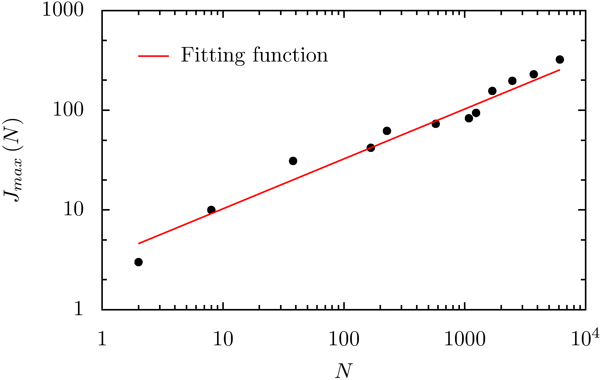
Figure 13: $J_{max}(N)$ for the background in Fig. 10 has a square root dependence on $N$ with a fitting function $3.25\sqrt{x}$.

.

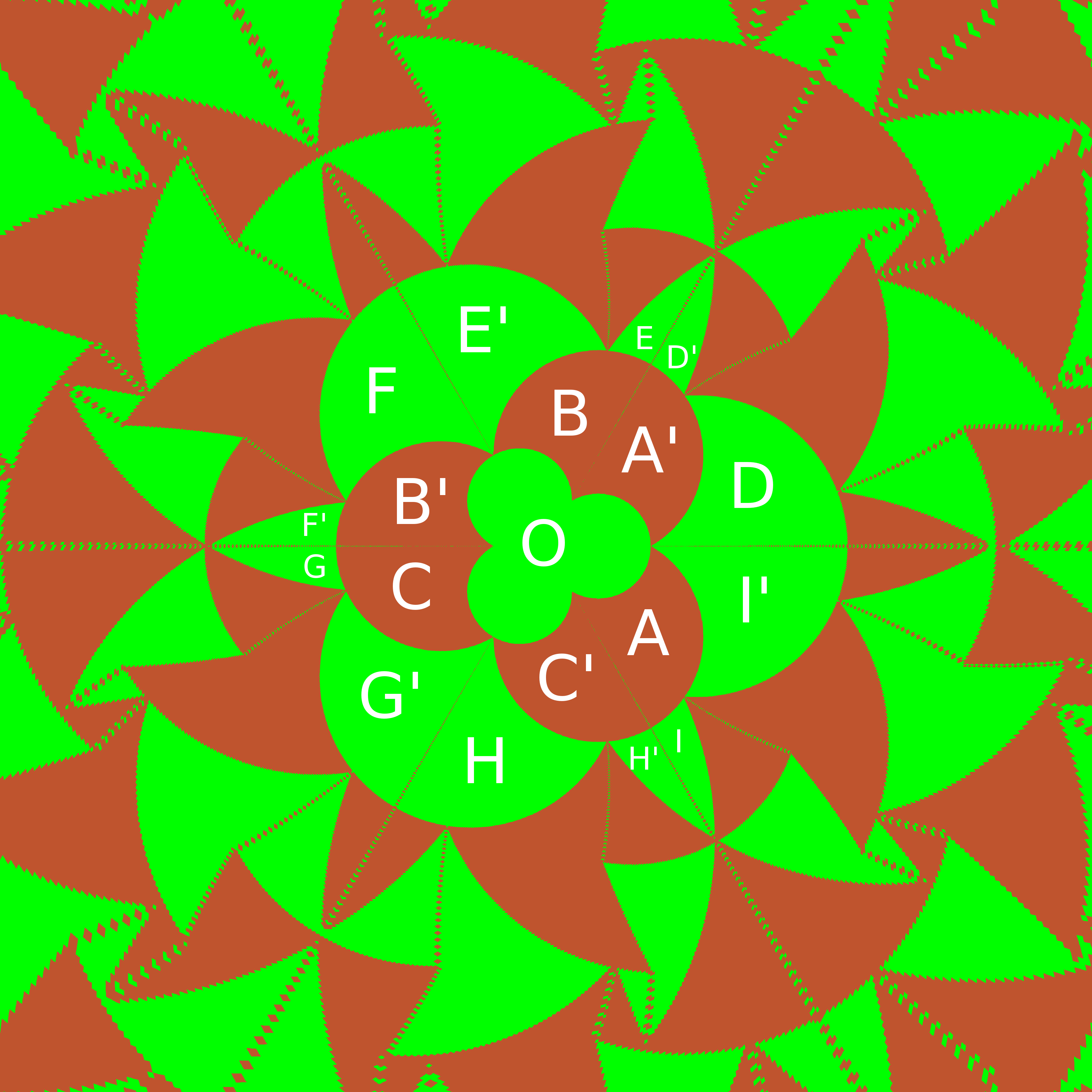
Figure 14: The $1/\mathbf{\bar{R}}$ transformation of the pattern in Fig. 11, where $\mathbf{\overline{R}}$ is the complex conjugate of $\mathbf{R}$. Labels are the same as used in Fig. 8(a).

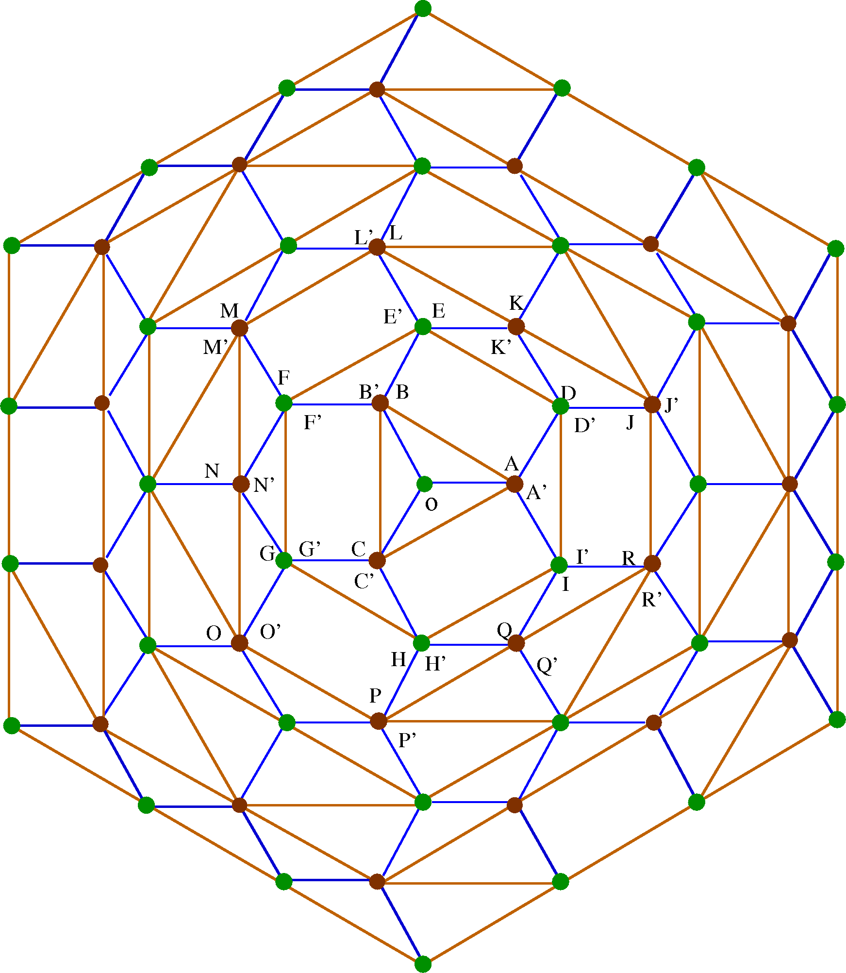
Figure 15: The adjacency graph of patches in the pattern in Fig. 11. The vertices corresponding to the brownish and greenish patches in the pattern are denoted by different colors. The pair of patches labeled by the alphabets and its corresponding primed alphabets in Fig. 8(a) are represented by same vertex on the graph.

We define scaled complex coordinates $\mathbf{r}=\mathbf{R}/N$, where $\mathbf{R}=p+q\omega$ is the complex coordinate of the site $\left(p,q\right)$. We define the rescaled toppling function for this pattern as

$$\phi\left(\mathbf{r}\right)=\lim_{N\rightarrow\infty}\frac{\sqrt{3}T_{N}\left(\mathbf{r}N\right)}{2N}.$$ (11)

Then it is easy to see that $\nabla\phi=\left(\partial_{\xi}\phi,\partial_{\eta}\phi\right)$ is equal to the mean flux of particles at $\mathbf{r}$. If we consider a small line element $d\mathbf{l}\equiv\left(d\xi,d\eta\right)$, then the net flux of particles across the line $d\mathbf{l}$ equals $N\nabla\phi\cdot d\mathbf{l}$. Then, the conservation of sand grains implies that the toppling function $T_{N}\left(\mathbf{R}\right)$ satisfies the equation

$$\nabla_{\circ}^{2}T_{N}\left(\mathbf{R}\right)=\delta z\left(\mathbf{R}\right)-N\delta\left(\mathbf{R}\right),$$ (12)

where $\nabla_{\circ}^{2}$ is the finite-difference operator on the lattice, corresponding to the Laplacian $\nabla^{2}$. It is easy to see that this implies that the scaled potential function $\phi$ satisfies the Poisson equation

$$\nabla^{2}\phi\left(\mathbf{r}\right)=\Delta\rho\left(\mathbf{r}\right)-\delta\left(\mathbf{r}\right),$$ (13)

where $\Delta\rho\left(\mathbf{r}\right)$ is the areal density of excess grains at $\mathbf{r}$. It is related to $\langle\Delta z\left(\mathbf{r}\right)\rangle$, the mean excess grain density per site by

$$\Delta\rho\left(\mathbf{r}\right)=\frac{2}{\sqrt{3}}\langle\Delta z\left(\mathbf{r}\right)\rangle.$$ (14)

The piece-wise linearity of $\phi$ simplifies the analysis of the pattern, significantly. The potential function can be characterized by only three parameters. Using Eq. (8), (9) and (11), for each patch $P$, we can find a pair of integers $\left(m,n\right)$ such that the potential in patch $P$ is characterized by

$$\phi\left(\mathbf{r}\right)=-\frac{1}{2\sqrt{3}}\left(\mathbf{D}_{m,n}\overline{\mathbf{r}}+\overline{\mathbf{D}}_{m,n}r\right)+f_{m,n},$$ (15)

where

$$\mathbf{D}_{m,n}=m+n\omega,$$ (16)

and $f_{m,n}$ is a real number, constant everywhere inside the patch. Here $\overline{z}$ denotes the complex conjugate of $z$.

Each patch is characterized by a complex number $\mathbf{D}_{m,n}$ which is the coefficient in the potential function $\phi\left(\mathbf{r}\right)$ of the patch. In the complex $\mathbf{D}$-plane, each patch with labels as in Fig. 8(a) can then be represented by a point. We connect two patches by a line if they share a common boundary. Then the resulting figure, shown in Fig. 15, is the adjacency graph of the patches.

We can determine the connectivity structure of this graph, without knowing the full potential function in each patch. We first take $1/\mathbf{\bar{R}}$ transformation of the pattern. This is shown in Fig. 14. Some of the bigger patches are denoted by capital alphabets in Fig. 8(a) and their corresponding patches on the transformed pattern in Fig. 14. The patches A and $\textbf{A}^{\prime}$ in Fig. 8(a) are adjacent to the outer region O through the same vertical boundary. Matching the values of the function $\phi(\mathbf{r})$ and fixing the discontinuity in its normal derivatives at the boundary, it is easy to see that $\phi(\mathbf{r})$ has the same functional form in the patches A and $\textbf{A}^{\prime}$. In fact, it is convenient to imagine that the boundary between O and A moved to the right by an infinitesimal amount, so that it does not touch the patches D and $\textbf{I}^{\prime}$, and then A and $\textbf{A}^{\prime}$ would actually join to form a single connected patch A. We thus consider A and $\textbf{A}^{\prime}$ as one patch, and both can be represented as one point on the $\mathbf{D}$-plane. Similarly, we identify B and $\textbf{B}^{\prime}$, C and $\textbf{C}^{\prime}$, etc. Then the adjacency graph can be constructed by joining the sites on the $\mathbf{D}$-plane, according to the adjacency of patches in Fig. 14.

It turns out that the patches corresponding to $m+n=2\left(\right.$mod$\left.3\right)$ do not appear in the pattern, and the adjacency graph, as shown in Fig. 15, is a hexagonal lattice with some extra edges shown in brown color. These extra edges connect all the vertices at same distance from the origin $\left(0,0\right)$ (in the $L^{1}$ metric), and also connect some of the diagonally opposite sites on the rectangular faces of the graph as shown in figure.

The charge density $\Delta\rho\left(\mathbf{r}\right)$ is zero inside the patches, and the excess grains due to addition are distributed along the patch boundaries, leading to nonzero line charge densities separating neighboring patches. Then the density function $\Delta\rho\left(\mathbf{r}\right)$ is a superposition of the line charge densities along the patch boundaries. There are three kinds of line charges of charge density $\lambda=-1/\sqrt{3}$, $1$, and $2/\sqrt{3}$.

From the electrostatic analogy, it is seen that $\phi\left(\mathbf{r}\right)$ is continuous across the common boundary between neighboring patches, and its normal derivative is discontinuous by an amount equal to the line charge density $\lambda$ along the boundary. Let $P$ and $P^{\prime}$ be the two neighboring patches with the equation of the boundary between them

$$\mathbf{r}=|\mathbf{r}|\exp\left(i\theta\right)+\mathbf{A},$$ (17)

such that the patch $P^{\prime}$ is on the left of the boundary. Then using the continuity condition, it is easy to show that

$$\mathbf{D}_{p^{\prime}}-\mathbf{D}_{p} = i\lambda\sqrt{3}\exp\left(i\theta\right)\rm{~{}and~{}}$$

$$f_{p^{\prime}}-f_{p} = Re[\overline{\mathbf{A}}\left(\mathbf{D}_{p^{\prime}}-\mathbf{D}_{p}\right)]/\sqrt{3},$$ (18)

where $\overline{\mathbf{A}}$ is the complex conjugate of $\mathbf{A}$. We note that, there are only six different types of patch boundaries in the pattern, with angle $\theta$ an integer multiple of $\pi/6$.

It is easy to check that the matching conditions along the edges of hexagonal lattice (denoted by blue solid line in Fig. 15) are sufficient to determine $D_{m,n}$ for all the vertices. The line charge density $\lambda=-1/\sqrt{3}$ for the patch boundaries corresponding to these edges. Also, the potential function $\phi=0$, for the vertex at the origin, and hence, $D$ and $f$ both vanishes. Then using the matching condition, it is easy to check that, the values of $D_{m,n}$ are consistent with the form in Eq. (16).

The function $f_{m,n}$ satisfies the discrete Laplace’s equation on the underlying hexagonal lattice of the adjacency graph i.e.

$$\sum_{m^{\prime},n^{\prime}}f_{m^{\prime},n^{\prime}}-3f_{m,n}=0\textrm{ ~{} ~{} ~{} for }\left(m,n\right)\neq 0,$$ (19)

where $\left(m^{\prime},n^{\prime}\right)$ denotes the three neighbors of the vertex $\left(m,n\right)$ on the hexagonal lattice. This can be checked from the concurrency condition of patch boundaries. For example consider the edges $\mathbf{OA}$, $\mathbf{DA^{\prime}}$ and $\mathbf{I^{\prime}A}$ on the adjacency graph. The corresponding patch boundaries in the pattern intersect at the same point (Fig. 8(a)). Then it is easy to check using the matching condition in Eq.(18) that,

$$f_{O}+f_{D}+f_{I}=3f_{A}.$$ (20)

Similar equations hold for the other vertices.

In the region outside the pattern, where none of the sites toppled, the potential function $\phi\left(z\right)=0$. This corresponds to $m=n=0$, and $f_{0,0}=0$. The solution of the Laplace’s equation with the above boundary condition can be written in the following integral form atkinson

$$f_{m,n}=\frac{I}{4\pi^{2}}\int_{-\pi}^{\pi}\int_{-\pi}^{\pi}\frac{1-\cos\left(k_{1}(2m-n)/3+k_{2}n\right)}{1-\left(\cos{2k_{2}}+2\cos{k_{1}}\cos{k_{2}}\right)/3}dk_{1}dk_{2},\rm{~{}~{}~{}~{}~{}~{}~{}}\textrm{ for $m+n=0$ (mod $3$)},$$ (21)

where $I$ is a normalizing constant, which determines the pattern up to a scale factor. For the sites with $m+n=1$ (mod $3$), $f_{m,n}$ are the average of those corresponding to the neighboring sites. As an example the potential function in region A, and $\textbf{C}^{\prime}$ is

$$\phi_{{}_{\textbf{A}}}(\mathbf{r}) = \frac{I}{3}-\frac{\xi}{\sqrt{3}},$$ (22)

$$\phi_{{}_{\textbf{C}^{\prime}}}(\mathbf{r}) = \frac{I}{3}+\frac{1}{\sqrt{3}}\left(\frac{1}{2}\xi+\frac{\sqrt{3}}{2}\eta\right),$$ (23)

where $\mathbf{r}=\xi+i\eta$, and $i=\sqrt{-1}$. Then the equation of the patch boundary between patches A and O is

$$\xi=I/\sqrt{3},$$ (24)

and that of the boundary between patches $\textbf{C}^{\prime}$ and O is

$$\sqrt{3}\xi+3\eta+2I=0.$$ (25)

Equivalently, the length of an edge of the bounding equilateral triangle of the pattern is equal to $2IN$, for large $N$.

The constant $I$ in Eq. (21) can be calculated using the form of the potential function near the site of addition. As noted, the function $\phi$ can be considered as the potential due to line charges along the patch boundaries and a point charge of unit amount at the origin. Then, close to the origin the solution diverges logarithmically as $\widetilde{\phi}\left(\mathbf{r}\right)=-\left(2\pi\right)^{-1}\log\left(|\mathbf{r}|\right)$, and the potential function is an approximation to this solution by a piece-wise linear function. Then, there are coordinates $\mathbf{r_{o}}$ inside each patch $\left(m,n\right)$ with $|m|+|n|$ large, where the $\phi$ and its first derivatives are equal to $\tilde{\phi}$ and its first derivatives, respectively. Then,

$$2\sqrt{3}\frac{\partial}{\partial\overline{\mathbf{r}}}\widetilde{\phi}\left(\mathbf{r}\right)|_{\mathbf{r_{o}}} \simeq -\mathbf{D}_{m,n}\rm{~{}~{}and~{}~{}}$$

$$-\frac{1}{2\sqrt{3}}\left\{\mathbf{D}_{m,n}\overline{\mathbf{r_{o}}}+\overline{\mathbf{D}}_{m,n}\mathbf{r_{o}}\right\}+f_{m,n} \simeq -\frac{1}{2\pi}\log\left(|\mathbf{r_{o}}|\right).$$

The above two equations imply

$$f_{m,n}\simeq\frac{1}{2\pi}\log\left(|m+n\omega|\right),$$ (27)

for $|m|+|n|$ large. Comparing it with the Eq. (21) for large $|m|+|n|$ we find that the numerical constant $I=1/\sqrt{3}$. This determines the potential function completely, and thus characterizes the pattern. For example, as in figure 8(a), the equation of the rightmost boundary of the pattern, using Eq. (24) is $x=N/3$. Equations of other boundaries of patches can be calculated similarly. For example, the reduced coordinates of the point where the patches $D$ and $D^{\prime}$ meet in Fig. 8(a), is determined by the condition that it is a common point of patches $D$, $J$ and $A^{\prime}$, and that the function $\phi$ is continuous.

$$f_{1,0}-\frac{1}{\sqrt{3}}\xi = f_{2,1}-\frac{1}{\sqrt{3}}\left(\frac{3}{2}\xi+\frac{\sqrt{3}}{2}\eta\right)$$ (28)

$$= f_{3,1}-\frac{1}{\sqrt{3}}\left(\frac{5}{2}\xi+\frac{\sqrt{3}}{2}\eta\right).$$

Then using the values $f_{1,0}=1/3\sqrt{3}$, $f_{2,1}=1/2\sqrt{3}$, and $f_{3,1}=7/6\sqrt{3}-1/\pi$ atkinson we get the reduced coordinates of this point as

$$\left(\xi,\eta\right)=\left(\frac{2}{3}-\frac{\sqrt{3}}{\pi},-\frac{1}{3\sqrt{3}}+\frac{1}{\pi}\right).$$ (29)

Equivalently, the height of the bounding equilateral triangle increases as $2N/\sqrt{3}\simeq 1.154N$. The estimated slope of the fitting line in Fig. 9 is 1.1, in reasonable agreement with the theory. However, even though the exact function $\Lambda(N)$ has large fluctuations of number theoretic origin, the estimated slope is noticeably lower than the calculated asymptotic value. To examine this discrepancy closer, we have plotted in Fig. 16 the discrepancy $2\Delta\Lambda=2N/\sqrt{3}-2\Lambda(N)$ as a function of $N$. We find that this appears to increase with $N$ as $N^{3/4}$, for large $N$. The reason for this behavior is not understood yet.

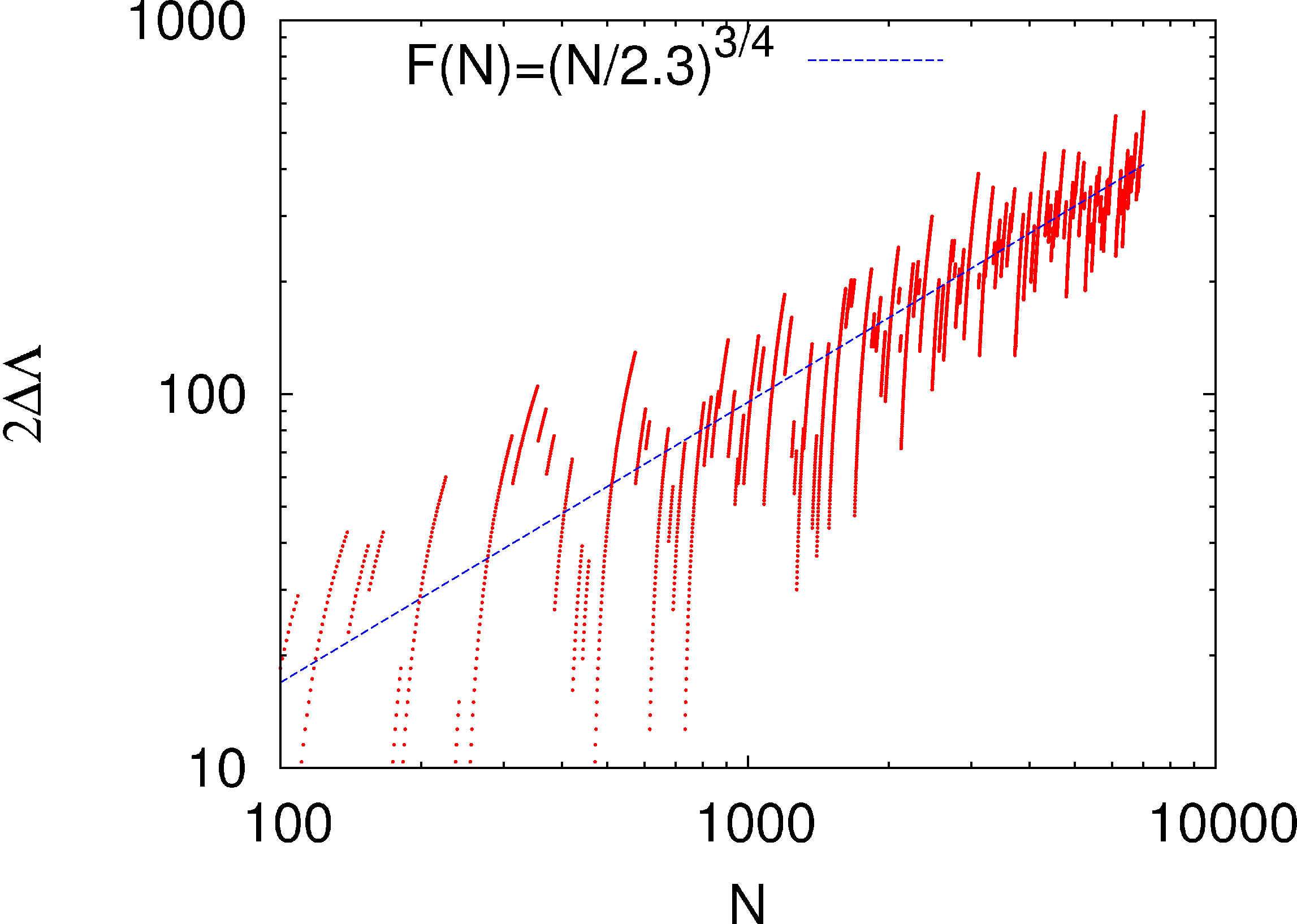
Figure 16: The discrepancy $2\Delta\Lambda$ between the actual height of bounding triangle, and the asymptotic value $2N/\sqrt{3}$ plotted as a function of $N$. The straight line shows a simple power-law fit with power $3/4$.

For backgrounds, with $l>1$, our numerical results suggest that there is a crossover length $R^{\star}(l)$, and initially, for $R<R^{\star}(l)$, the avalanches grow “explosively” in size. As a result, the number of particles inside a disc of radius $R^{\star}$ in the final pattern is less than that in the initial background. The net flux of particles going out of the disc increases with $R$ until the radius becomes of order $R^{\star}$. After this, the large-scale properties of the pattern are the same as that of $l=1$ pattern, with the number of particles added $A_{\ell}N$, where $A_{\ell}$ is an $\ell$-dependent constant. In particular, the size of the pattern is $A_{\ell}$ -times the size of the pattern for $l=1$ with same $N$. The crossover length $R^{\star}$ is expected to grows as $\sqrt{N}$.

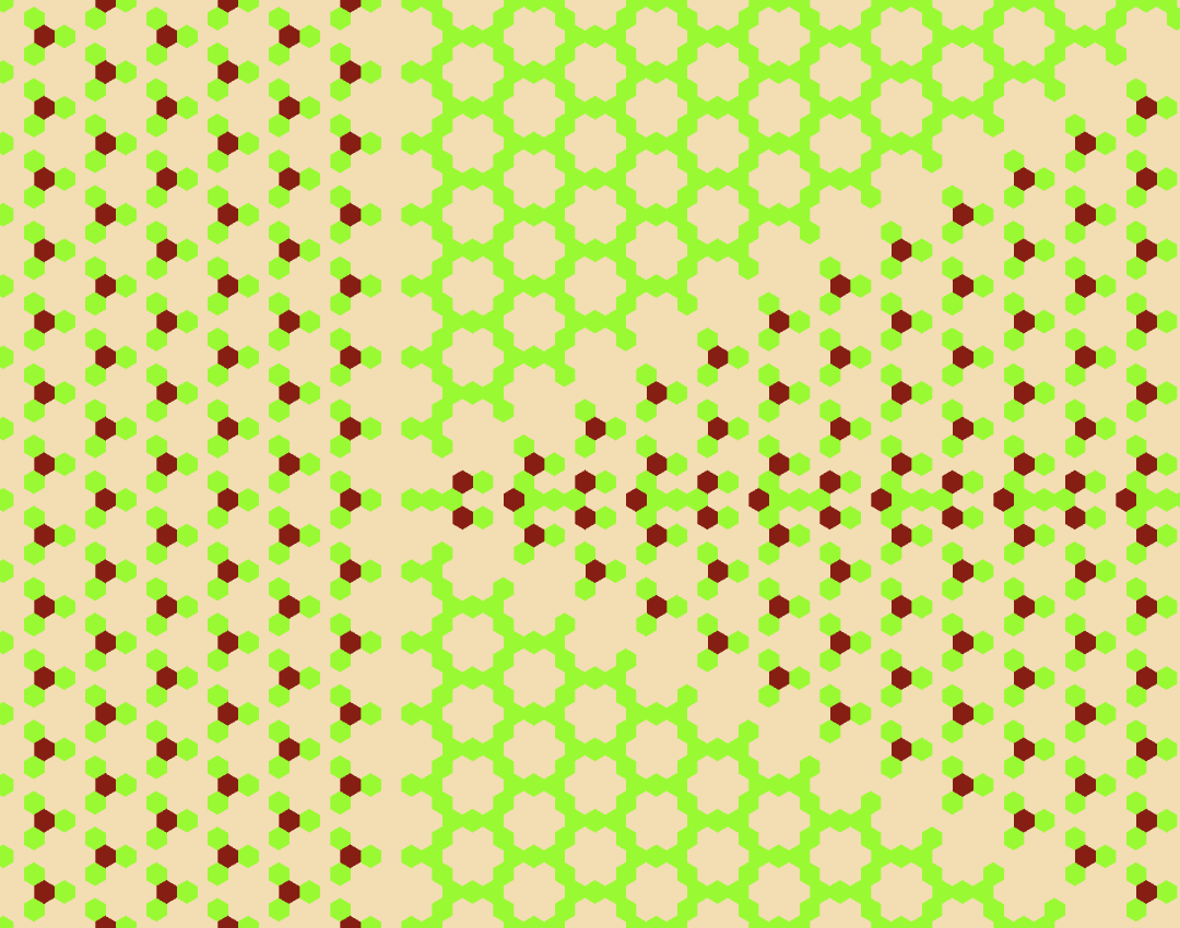
Figure 17: An example of five patches meeting at a point, for a pattern on the background of Class $I$, $\ell=2$. It is easy to check that the line charge density for the vertical boundary $\lambda=-1/\sqrt{3}$, same as in Fig. 12. The color code is same as in Fig. 11.

For a background with $\ell>1$, the basis vectors at the unit cell are $\ell\hat{e}_{1}$ and $\ell\hat{e}_{2}$, where $\hat{e}_{1}$, $\hat{e}_{2}$ are the basis vectors for $\ell=1$ background (see Eq. (9)). Then the reciprocal basis vectors are $\hat{g}_{1}/\ell$ and $\hat{g}_{2}/\ell$. From the observed patterns, we find that the line charge densities remain same for any $\ell$ (see Fig. 17 for an example of the patch boundaries). This implies that $n_{1}$ and $n_{2}$ in eq. (8) are constrained to be multiples of $l$. Writing $n_{1}=lm$, $n_{2}=ln$, we see that the patches can be labeled by the same pair of integers $\left(m,n\right)$ as in the $\ell=1$ case, and the potential function $\phi_{(l)}\left(\mathbf{r}\right)$ for general $l$ is related to the $l=1$ case by simple scaling:

$$\phi_{(\ell)}\left(\mathbf{r}\right)=A_{\ell}\phi_{(1)}\left(\frac{\mathbf{r}}{A_{\ell}}\right),$$ (30)

where $A_{\ell}$ is a scale factor. For $\ell=2$, $3$, $4$ and $5$ the values of $A_{\ell}$ are approximately $2.34$, $3.38$, $4.41$ and $5.37$, respectively. We note that $A_{\ell}$ increases approximately linearly with $\ell$.

VI Non-compact patterns with exponent $\alpha<1$

On the F-lattice, after some experimentation, we found that the background pattern having the periodicity of the tiling of plane with tilted rectangles, shown in Fig. 18, produces patterns with interesting non-compact growth. We studied rectangles with aspect ratio $l:(l+1)$, and the rectangles are tilted by $45^{\circ}$ to the x-axis. Two such periodic backgrounds are shown in Fig. 19. In these background patterns, the sites with height zero, are arranged along the boundaries of tilted rectangles with two possible orientations, and rest of the sites have height one. The stable height-patterns generated by adding $N$ particles and relaxing the configuration on these two backgrounds are shown in Fig. 20 and Fig. 21, respectively. The growing boundaries of the patches in the patterns are shown, in terms of the $Q$ variables, in Fig. 22 and 23, respectively. Again, we see that the patch boundaries are straight lines, with rational slopes. The plot of diameter $2\Lambda$ vs N, for these two patterns are shown in Fig. 24. We see that the growth exponent $\alpha$ is approximately $0.6$ for figure 20 and $0.725$ for figure 21. In general, value of the exponent $\alpha$ is in range $1/2<\alpha<1$, and approaches value $1$ as density $\rho_{o}$ of the background becomes close to $1$.

There are unresolved areas of apparent solid color in the patterns, taking up a sizable fraction of the total area, e.g., two large regions of red color on both sides of Fig. 22. In these regions, the pattern appears to be complex, suggesting either a large number of patch boundaries, or patches of non-zero areal excess charge density. However, the fractional area of these regions decreases with larger $N$. Also on comparing patterns with different $l$, we have seen that the fractional area of such regions decreases as $l$ increases. A more detailed study of these patterns seems like an interesting problem for future investigations.

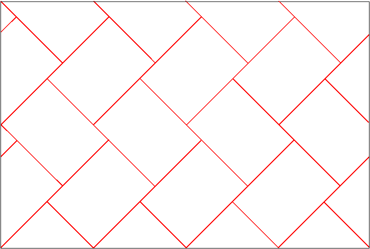
Figure 18: A schematic representation of the periodic tiling of the plane using tilted rectangles. Background height patterns with such periodicities on the F-lattice give rise to non-compact growth with the growth-exponent between $1/2$ and $1$

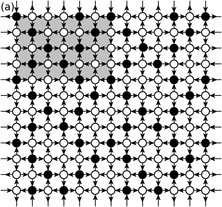
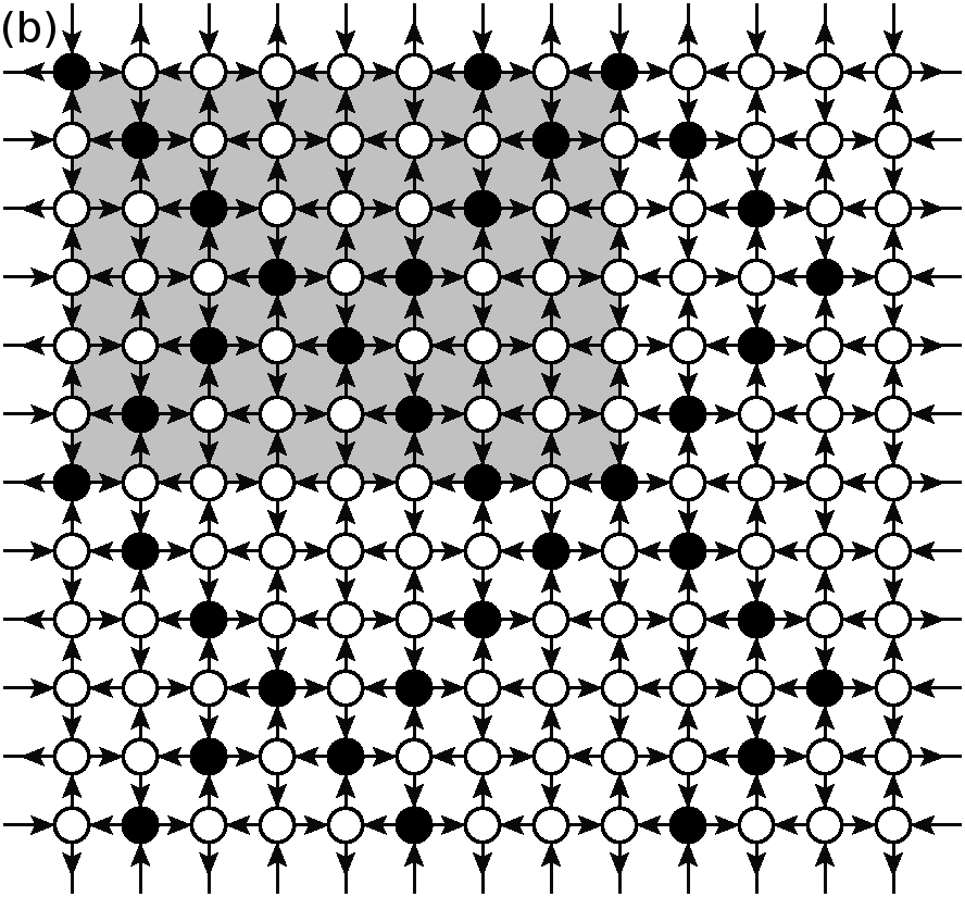
Figure 19: The two backgrounds studied on the F-lattice. Unit cells of the periodic distribution of particles are shown by gray rectangular shades. The filled circles represent height $0$ and unfilled ones $1$.

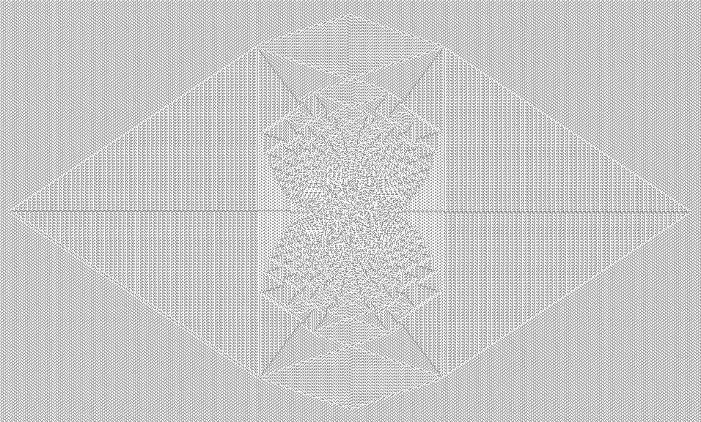
Figure 20: The pattern produced on the first background in Fig. 19, by adding $N=2200$ grains at a single site, and relaxing the configuration. Color code: White$=1$ and Black$=0$. Details can be viewed in the electronic version using zoom in.

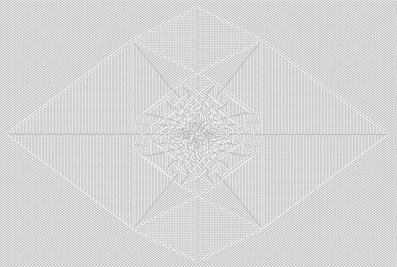
Figure 21: The pattern produced on the second background in Fig. 19 by adding $N=600$ grains at a single site, and relaxing the configuration. Color code: White$=1$ and Black$=0$. Details can be viewed in the electronic version using zoom in.

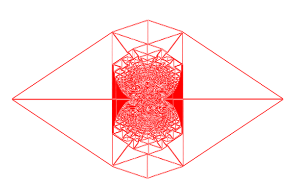
Figure 22: The pattern in terms of $Q(r)$, showing the boundaries of patches corresponding to Fig. 20. Color code: White$=0$ and Red$=$Non-zero. Details can be viewed in the electronic version using zoom in.

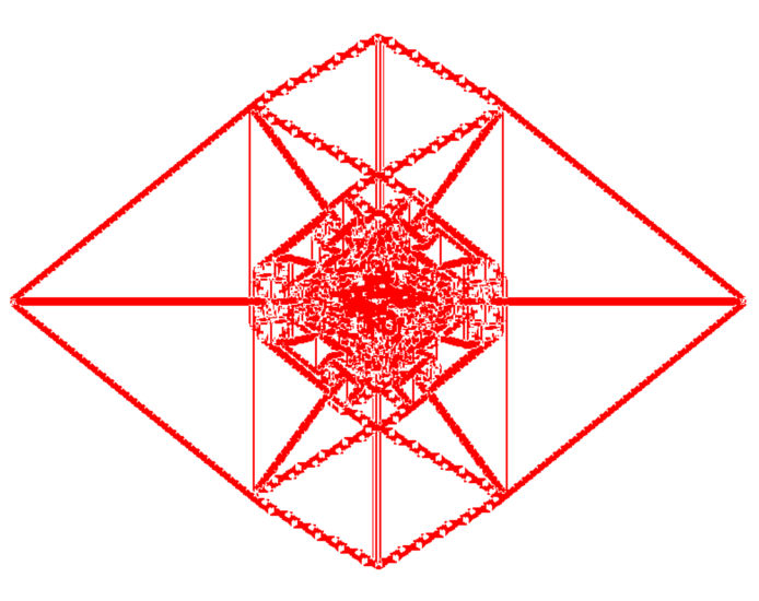
Figure 23: The pattern in terms of $Q(r)$, showing the boundaries of patches corresponding to Fig. 21. Color code: White$=0$ and Red$=$Non-zero. Details can be viewed in the electronic version using zoom in.

VII Summary and concluding remarks

In this paper, we have studied two dimensional patterns formed in Abelian sandpile models by adding particles at one site on an initial periodic background, where the diameter of the pattern grows as $N^{\alpha}$, with $\alpha>1/2$. Using some features observed in the pattern of adjacency of patches as an input, we are able to determine the exact asymptotic pattern in the specific case with $\alpha=1$, on a class $I$ background.

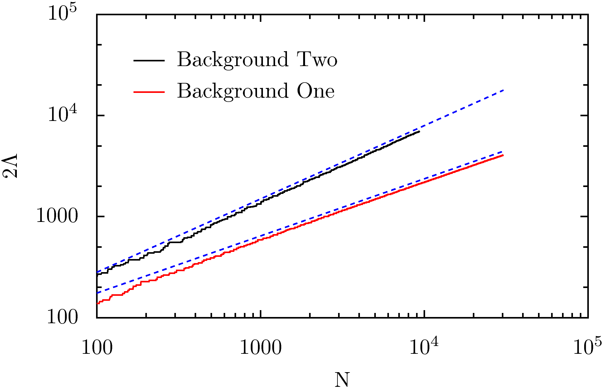
Figure 24: The change in diameter as a function of $N$, for the patterns on the two backgrounds in Fig. 19. The numerical results fit well with straight lines of slope $0.6$ and $0.725$, for the backgrounds one and two, respectively.

The patterns on class $II$ backgrounds can also be characterized similarly. As noted earlier, some of the patches split into smaller parts. By using the $1/\overline{\mathbf{R}}$ transformation, we can again determine the structure of the adjacency graph. The graph for the pattern in Fig. 8(b) is shown in Fig. 25. It is a periodic lattice where half of the vertices of the hexagonal lattice are replaced by $3$ vertices (colored in brown). The exact D-values for different patches can be easily determined. The determination of $f_{m,n}$ for this pattern then requires the solution of the Laplace’s equation on this graph. It can be shown that a slight alteration of the graph, by drawing the missing edges in the small triangles shown in pink colors, does not change the pattern. Then the solution of the Laplace’s equation can be reduced to the solution of a resistor network on this modified graph. The later can be further reduced to the resistor network on a hexagonal lattice, discussed by Atkinson et.al. atkinson , using the well-known $Y-\Delta$ transformation. We omit details of the analysis here.

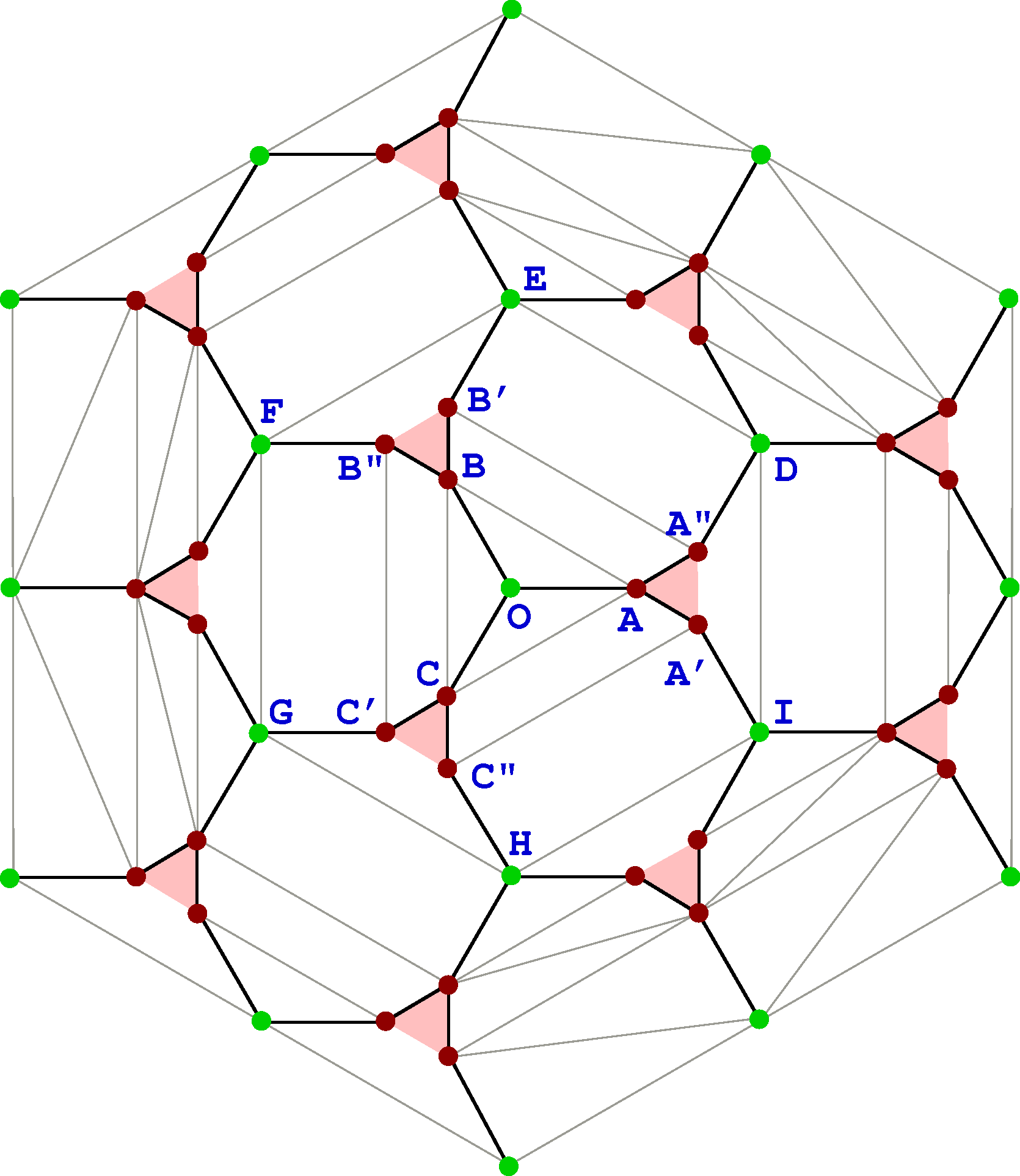
Figure 25: The adjacency graph of the patches in the pattern in Fig. 8(b). The vertices corresponding to the brownish and greenish patches in the pattern (Fig.7) are denoted by different colors.

An important feature of the non-compact patterns is that, it can be characterized by a piece-wise linear function. This characterization is simpler than that of the patterns with compact growth, where one requires piece-wise quadratic polynomials. We have shown that there are infinitely many backgrounds, on which the patterns have non-compact growth. It would be desirable to determine the exact value of $\alpha$ for different backgrounds showing non-compact growth studied in Sec. VI.

Another interesting question is a possible connection of this problem to tropical algebra tropical . In tropical mathematics, one defines operations similar to ‘addition’ and ‘multiplication’ (denoted by $\oplus$ and $\otimes$ here) by

$$a\oplus b = \textrm{max}\left\{a,b\right\},$$

$$a\otimes b = a+b,$$ (31)

where $a$, $b$ are real parameters. Familiar properties of addition and multiplication operators, like commutativity, associativity, existence of identity, distributive property continues to hold in the new definition. One can then define polynomials in several variables. The graph of a tropical polynomial is a piecewise linear function which is also convex. For example, consider the tropical function

$$f(x)=a\otimes x^{2}\oplus b\otimes x\oplus c.$$ (32)

In terms of standard algebra

$$f(x)=max\left\{a+2x,bx,c\right\}.$$ (33)

The graph corresponding to this function is shown in Fig. 26

We note that for the pattern discussed in section $4$, the potential function is piece-wise linear. It seems plausible that tropical polynomials may be useful to describe this function. In fact, tropical geometry have been discussed as possibly related to sandpile models norine ; propp2 . For small values of $N$, our numerical study showed that $\phi$ is convex, if restricted to one sextant. However, for larger $N$, as shown in Fig. 27, we see that $\phi$ is not convex even within one sextant. We conclude that it is not possible to represent the potential $\phi$ as a simple tropical polynomial.

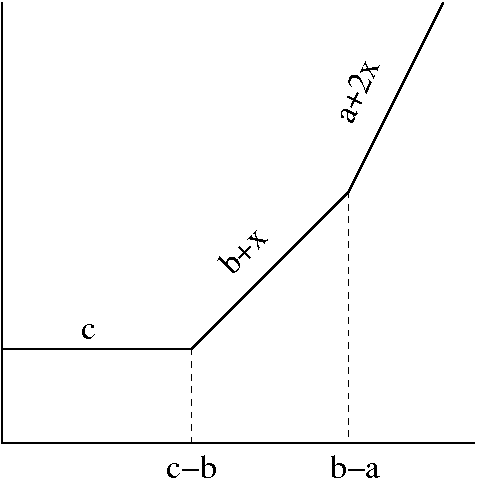
Figure 26: Graph corresponding to the tropical function in equation (32)

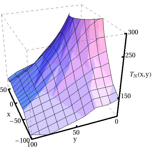
Figure 27: (Color online.) Three dimension plot of the integer toppling function $T_{N}\left(x,y\right)$ for a triangular pattern like in Fig. 11, but with $N=800$. The plot shows a zoomed-in section in the region $y\geq 0$ and $y+\sqrt{3}x\geq 0$.

Appendix A Relation to the theory of discrete analytic functions

The sandpile patterns we studied are characterized in terms of discrete analytic functions (DAF) on different discretizations of the complex plane. For the pattern in Fig. 11, it is the DAF on a hexagonal lattice, which increases logarithmically at large distances as in Eq. (27).

Studies of DAF started with the work of Kirchhoff on resistor networks hu ; cserti ; Doyle , and has been studied subsequently by many others duffin ; mercat . However, we have not encountered any work on DAF on many sheeted Riemann surfaces. In the following we present a way to determine DAF on a square discretization of Riemann surfaces.

Consider a square grid of points $z=m\epsilon+in\epsilon$, where $m,n$ are integers and $\epsilon$ is the lattice spacing. Let $f\left(m\epsilon,n\epsilon\right)$ be a complex function defined at every site on the grid. The function $f$ is defined to be discrete analytic laszlo if it satisfies the discrete Cauchy Riemann condition

$$\frac{f\left(z_{3}\right)-f\left(z_{1}\right)}{z_{3}-z_{1}}=\frac{f\left(z_{4}\right)-f\left(z_{2}\right)}{z_{4}-z_{2}},$$ (34)

at all elementary squares on the grid as shown in Fig. 28.

In complex analysis, simple examples of analytic functions are $z^{n}$, and any polynomial of $z^{n}$ is also analytic. For DAF, it is clear, using the linearity of equation (34), that sum of DAF is also discrete analytic. However, not all positive integer powers of $z$ are discrete analytic. It is easy to check that the functions $1$, $z$, $z^{2}$, $z^{3}$ are discrete analytic, but $z^{4}$ is not. We can however construct polynomial functions of $Re(z)$ and $Im(z)$, that are discrete analytic. Two such examples are $z^{4}-z\overline{z}\epsilon^{2}$ and $z^{5}-5z^{2}\overline{z}\epsilon^{2}/2$.

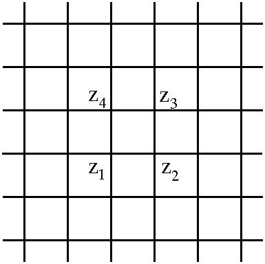
Figure 28: A square grid on the complex plane.

We define a function $F_{n}(z,\epsilon)$ as a homogeneous polynomial in $z$, $\overline{z}$ and $\epsilon$, of degree $n$, which is a DAF. Using homogeneity, we have

$$F_{n}(z,\epsilon)=a^{n}F_{n}(\frac{z}{a},\frac{\epsilon}{a}),$$ (35)

and then using $a=\epsilon$, we can express $F_{n}(z,\epsilon)$ in terms of $F_{n}(z,1)$. This fixes $F_{n}(z,\epsilon)$ up to a multiplicative constant. The normalization is fixed by requiring that as $\epsilon$ tends to zero, $F_{n}\left(z,\epsilon\right)\rightarrow z^{n}$. Then using Cauchy Riemann conditions it is easily seen that $F_{n}(z,\epsilon)$, for all integers $n\geq 0$, has a series expansion in $\epsilon^{2}$ of the form

$$F_{n}(z,\epsilon)=z^{n}\left[1+\frac{\epsilon^{2}}{z^{2}}g_{1}^{(n)}(\frac{\overline{z}}{z})+\frac{1}{2!}\frac{\epsilon^{4}}{z^{4}}g_{2}^{(n)}(\frac{\overline{z}}{z})+\cdots\right],$$ (36)

where

$$g_{1}^{(n)}(x) = -\frac{1}{n-3}\binom{n}{4}x,$$ (37)

$$g_{2}^{(n)}(x) = \frac{7!}{(4!)^{2}}\frac{1}{n-6}\binom{n}{7}x^{2},$$ (38)

$$g_{3}^{(n)}(x) = -\frac{10!}{(4!)^{3}}\frac{1}{n-9}\binom{n}{10}x^{3}-\frac{27}{n-7}\binom{n}{8}x,$$

and so on. For an integer $n$, this series will terminate after a finite number of terms, and all of them can be determined iteratively.

It is possible to analytically continue the functions for rational values of $n$. For example,

$$g_{1}^{(n)}(x)=-\frac{\Gamma(n+1)}{4!\Gamma(n-2)}x.$$ (40)

Then, this analytic continuation of $F_{n}(z,\epsilon)$ provides us the discrete analytic functions which in the limit $|z|\rightarrow\infty$ grows as $z^{n}$, for any real positive values of $n$. It is interesting to note that the function $D_{m,n}$, used in myepl to characterize the pattern in Fig. 2(b), is equal to $F_{1/2}(z=m+in,\epsilon=1)$, up to a multiplicative constant. The patterns in the presence of a line of sinks, or near wedges studied in myjsp involve other rational values. For example, for the pattern near a line sink, one requires the function $F_{1/3}(z,1)$.

References

- [1] D. Dhar. Theoretical studies of self-organized criticality. Physica A: Statistical and Theoretical Physics, 369(1):29–70, 2006.
- [2] F. Redig. Mathematical aspects of the abelian sandpile model, Les Houches lecture notes. http://www.math.leidenuniv.nl/redig/sandpilelectures.pdf, 2005.
- [3] L. S. Schulman and P. E. Seiden. Statistical mechanics of a dynamical system based on Conway’s game of life. Journal of Statistical Physics, 19:293–314, 1978.
- [4] H. J. Herrmann. Geometrical cluster growth models and kinetic gelation. Physics Reports, 136(3):153 – 224, 1986.
- [5] T. A. Witten and L. M. Sander. Diffusion-limited aggregation. Phys. Rev. B, 27(9):5686–5697, 1983.
- [6] Barabasi L. and Stanley H. E. Fractal Concepts in Surface Growth. Cambridge University Press, 1995.
- [7] S. H. Liu, T. Kaplan, and L. J. Gray. Geometry and dynamics of deterministic sand piles. Phys. Rev. A, 42(6):3207–3212, 1990.
- [8] D. Dhar. Studying Self-Organized Criticality with Exactly Solved Models. arXiv:cond-mat/9909009, 1999.
- [9] Y. Le Borgne and D. Rossin. On the identity of the sandpile group. Discrete Math., 256(3):775–790, 2002.
- [10] A. Fey and F. Redig. Limiting shapes for deterministic centrally seeded growth models. Journal of Statistical Physics, 130:579–597, 2008.
- [11] L. Levine and Y. Peres. Strong spherical asymptotics for rotor-router aggregation and the divisible sandpile. Potential Analysis, 30:1–27, 2009.
- [12] S. Ostojic. Patterns formed by addition of grains to only one site of an abelian sandpile. Physica A: Statistical Mechanics and its Applications, 318(1):187 – 199, 2003.
- [13] D.B. Wilson. Sandpile aggregation pictures on various lattices. http://research.microsoft.com/en-us/um/people/dbwilson/sandpile/.
- [14] M. Creutz. Abelian sandpiles. Comput. Phys., 5:198–203, 1991.
- [15] S. Caracciolo, G. Paoletti, and A. Sportiello. Explicit characterization of the identity configuration in an abelian sandpile model. Journal of Physics A: Mathematical and Theoretical, 41(49):495003, 2008.
- [16] G.F. Lawler, M. Bramson, and D. Griffeath. Internal diffusion limited aggregation. Ann. Probab., 20(4):2117–2140, 1992.
- [17] V. B. Priezzhev, Deepak Dhar, Abhishek Dhar, and Supriya Krishnamurthy. Eulerian walkers as a model of self-organized criticality. Physical Review Letters, 77:5079–5082, 1996.
- [18] L. Levine and Y. Peres. Spherical asymptotics for the rotor-router model in . Indiana Univ. Math. J., 57:431–450, 2008.
- [19] A.E. Holroyd, L. Levine, K. Meszaros, Y. Peres, J. Propp, and D.B. Wilson. Chip-firing and rotor-routing on directed graphs. In In and Out of Equilibrium II, Progress in Probability, volume 60, 2008.
- [20] J. Gravner and J. Quastel. Internal DLA and the stefan problem. Ann. Prob., 28(4):1528–1562, 2000.
- [21] L. Levine and Y. Peres. Scaling limits for internal aggregation models with multiple sources. Journal d’Analyse Mathématique, 111(1):151–219, 2010.
- [22] A. Fey and H. Liu. Limiting shapes for a non-abelian sandpile growth model and related cellular automata. ArXiv e-prints, 2010.
- [23] D. Dhar, T. Sadhu, and S. Chandra. Pattern formation in growing sandpiles. EPL, 85(4):48002, 2009.
- [24] T. Sadhu and D. Dhar. Pattern formation in growing sandpiles with multiple sources or sinks. Journal of Statistical Physics, 138:815–837, 2010.
- [25] T. Sadhu and D. Dhar. The effect of noise on patterns formed by growing sandpiles. Journal of Statistical Mechanics: Theory and Experiment, 2011(03):P03001, 2011.
- [26] A. Fey, L. Levine, and Y. Peres. Growth rates and explosions in sandpiles. Journal of Statistical Physics, 138:143–159, 2010.
- [27] D. Atkinson and F. J. Van Steenwijk. Infinite resistive lattices. Am. J. Phys., 67(6):486–492, 1999.
- [28] D. Dhar. The abelian sandpile and related models. Physica A: Statistical Mechanics and its Applications, 263(1-4):4 – 25, 1999.
- [29] D. Speyer and B. Sturmfels. Tropical mathematics. Mathematics Magazine, 82:163–173(11), 2009.
- [30] Matthew Baker and Serguei Norine. Riemann-roch and abel-jacobi theory on a finite graph. Advances in Mathematics, 215(2):766 – 788, 2007.
- [31] L. Levine and J. Propp. What is a sandpile? Notices of the AMS, 57:976–979, 2010.
- [32] F. Y. Wu. The potts model. Rev. Mod. Phys., 54(1):235–268, 1982.
- [33] József Cserti. Application of the lattice green’s function for calculating the resistance of an infinite network of resistors. Amer. J. Phys., 68(10):896–906, 2000.
- [34] Peter G. Doyle and J. Laurie Snell. Random Walks and Electric Networks. Mathematical Association of America, Washington, DC, 1984.
- [35] R. J. Duffin. Basic properties of discrete analytic functions. Duke Mathematical Journal, 23(2):335–363, 1956.
- [36] C. Mercat. Discrete Riemann surfaces and the Ising model. Commun. Math. Phys., 218:177–216, 2001.
- [37] L. Lovsz. Discrete Analytic Functions: An Exposition., pages 241–273. Int. Press, Somerville, MA, second edition, 2004.