Diffusion dynamics in a Tevatron store

Abstract

A separator failure during a store in 2002 led to a drop in luminosity, to increased emittance growth and to a drop in beam lifetimes. We show that a simple diffusion model can be used to explain the changes in emittance growth and beam lifetimes.

1 Introduction

Emittance growth of beams when they are in collision occurs due to many sources: beam-beam interactions, magnetic nonlinearities, intra-beam scattering, scattering off the residual gas and possibly others. The dynamics of the emittance growth is complicated and it depends strongly on the tunes. It is not always clear that the dynamics can be described by a diffusion process at all particle amplitudes in each beam. However in one store early in Run II, there was a sudden drop in a separator voltage in the Tevatron and the subsequent enhanced emittance growth and intensity lifetime drop could be described by a simple diffusion model. In this report we analyze the luminosity drop, compare the measured value with the expected drop and analyze the change in beam lifetimes. We show how a simple model of diffusive emittance growth and a change in physical aperture provides a quantitative explanation for the change in lifetimes.

2 Separator failure and luminosity drop

After about 13.5 hours into store 1253 (April 26, 2002), the voltage on the bottom plate of the horizontal separator at A49 dropped from a value of -90kV to -25kV. This immediately lowered the luminosity at CDF and D0. The emittance growth rate increased and the lifetimes of both protons and anti-protons fell. Table 1 shows some of the key beam and machine parameters.

$\beta_{x}^{*}$ at CDF, D0	0.35m
Horizontal tune	$\nu_{x}$ = 20.585
Observed Luminosity drop at CDF	41.4%
Observed Luminosity drop at D0	42.3%
Total proton beam intensity before drop	5.78 $\times 10^{12}$
Initial emittances (p and pbar) $\epsilon_{x},\epsilon_{y}$ [$\pi$mm-mrad]	22, 21
Estimated final emittances $(p,\bar{p})$ [$\pi$mm-mrad]	(26 - 30, 25 - 29)
Average emitt. growth rate [$\pi$mm-mrad/hr]	0.3-0.5
Length of store [hrs]	15
Location of BPMs nearest to CDF [m]	7.5 upstream and downstream
BPM upstream of CDF	$\beta_{x}$= 159.5 m, $\psi_{x}=2\pi\times$ 20.337
BPM downstream of CDF	$\beta_{x}$= 160.44 m, $\psi_{x}=2\pi\times$ 0.238
A49H Separator	$\beta_{x}$= 867.67m, $\psi_{x}=2\pi\times$ 20.329

Table 1: Relevant beam and machine parameters in Store 1253.

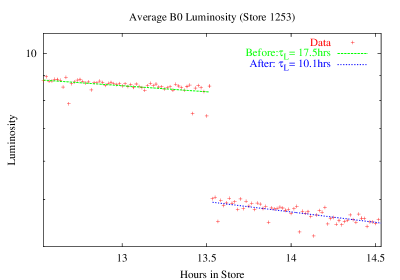
Figure 1: Average CDF Luminosity (raw data) and fits before and after the separator failure. The luminosity at CDF dropped by 41% right after the separator failure.

Figure 1 shows the measured luminosity drop at the CDF experiment after the separator failure. The luminosity at D0 dropped by a similar amount.

2.1 Closed orbit shift at CDF and D0

Here we estimate the orbit change as a consequence of the change in separator voltage at A49. The shift in the closed orbit due to a kick $\Delta\theta$ can be found from

$$\Delta x(s)=\frac{\Delta\theta\sqrt{\beta_{sep}\beta(s)}}{2\sin\pi\nu_{x}}\cos[\pi\nu_{x}-|\psi(s)-\psi_{sep}|]$$ (1)

where $\beta_{sep},\beta(s)$ are the beta functions at the separator and at $s$ respectively, $\psi(s),\psi_{sep}$ are the phase advances from a reference point to $s$ and the separator respectively and $\nu_{x}$ is the horizontal tune. The kick resulting from the electric field ${\cal E}$ across the separator plates of length $L$ on a particle of energy $E$ is given approximately by $\Delta\theta={\cal E}L/E$. At 980 GeV, a change in voltage of 65 kV across the separator plates with a gap of 5cm results in a kick of

$$\Delta\theta=3.41\mu{\rm rad}$$ (2)

Using the above expressions we find that the proton’s horizontal closed orbit would move by

$$\Delta x_{co}(CDF)|_{sep}=29.9\mu{\rm m},\;\;\;\;\;\;\;\;\Delta x_{co}(D0)|_{sep}=-30.3\mu{\rm m}$$ (3)

The orbit separation $d_{co}$ between the beams at the IPs would be twice the above value if the protons and anti-protons undergo the same but opposite changes in orbit. However the beam-beam kick with separated beams also induces an orbit shift and this will be larger for the anti-protons. Calculation of the beam-beam induced orbit kick requires that we know the separation between the beams, but that is precisely the quantity that we want to predict. We will approximate the beam-beam induced orbit kick by assuming that the beam separation is twice the shift in the proton orbit. In that case, the beam-beam kick assuming round Gaussian beams is

$$\Delta x^{\prime}_{bmbm}=8\pi\xi\epsilon\frac{x+d}{(x+d)^{2}+y^{2}}\left\{1-\exp[-\frac{(x+d)^{2}+y^{2}}{2\sigma^{2}}]\right\}$$ (4)

where $\xi$ is the beam-beam parameter, $\epsilon$ is the un-normalized rms emittance and $d$ is the horizontal separation between the beams. Extracting the dipole part of the kick,

$$\Delta x^{\prime}_{bmbm}(0,0)=8\pi\xi\epsilon\frac{1}{d}\left\{1-\exp[-\frac{d^{2}}{2\sigma^{2}}]\right\}$$ (5)

Since the sign of the pbar orbit offsets at CDF and D0 due to the separators have opposite signs, the kicks experienced by the anti-protons due to the dipole beam-beam kicks at CDF and D0 have opposite signs. Hence the contribution of the beam-beam kicks at CDF and D0 to the orbit shift at CDF is

$$\Delta x_{co}(CDF)|_{BB}=\frac{\beta^{*}|\Delta x^{\prime}_{bmbm}|}{2\sin\pi\nu_{x}}\left[\cos\pi\nu_{x}-\cos(\pi\nu_{x}-|\psi_{x}(D0)-\psi_{x}(CDF)|)\right]$$ (6)

We have assumed here that the beta functions at the IPs did not change much.

From the average proton bunch intensity of $N_{p}=1.61\times 10^{11}$ and an expected proton emittance of 30$\pi$ at this stage of the store (this number is found later by a self-consistent calculation), we find that the beam-beam parameter for anti-protons at this stage was $\xi=3.92\times 10^{-3}$. Hence the beam-beam kick using the value of the orbit offset found in Equation (3) is

$$\Delta x^{\prime}_{bmbm}(CDF)=5.14\mu{\rm rad}$$ (7)

while at D0, the kick has the opposite sign. Note that this kick is larger than the kick due to the change in the separator voltage, cf. Eq. (2). However because of the small beta function at the IPs, the change in orbit due to these beam-beam kicks is quite small,

$$\Delta x_{co}(CDF)|_{BB}=-0.42\mu{\rm m}$$ (8)

using Equation (6). This is almost two orders of magnitude smaller than the orbit shift due to the separator and can be neglected.

The predicted luminosity in terms of the luminosity ${\cal L}_{0}$ before the separator failure is found from

$${\cal L}={\cal L}_{0}\exp[-\frac{d_{co}^{2}}{2(\sigma_{p}^{2}+\sigma_{\bar{p}}^{2})}]$$ (9)

where $d_{co}\approx 2\Delta x_{co}|_{sep}$. This calculation depends on the emittances at the time of the failure. With the initial emittances and average emittance growth rates shown in Table 1, the proton emittances after 13.5 hrs were likely to be in the range (26, 30)$\pi$mm-mrad and anti-proton emittances (25, 29)$\pi$mm-mrad. We find using the orbit shifts in Eq. (3) (virtually the same at CDF and D0) and the low and high end of the emittance range,

$$\frac{\Delta{\cal L}}{\cal L}=0.47,\;\;\;\;(\epsilon_{p}=26,\epsilon_{pbar}=25)$$

$$\frac{\Delta{\cal L}}{\cal L}=0.42\;\;\;\;(\epsilon_{p}=30,\epsilon_{pbar}=29)$$ (10)

These values are to be compared with the observed relative drops in luminosity of 0.414 at CDF and 0.423 at D0. This suggests that the emittances were more likely at the higher end of the quoted range.

Another test of the optics is to propagate the measured orbit changes at the BPMs closest to CDF back to CDF using

$$\Delta x(s_{2})=\sqrt{\frac{\beta(s_{2})}{\beta(s_{1})}}\frac{\cos[\pi\nu-|\psi(s_{2})-\psi_{sep}|]}{\cos[\pi\nu-|\psi(s_{1})-\psi_{sep}|]}\Delta x(s_{1})$$ (11)

where $s_{1}$ is the location of a BPM and $s_{2}$ is the location of an IP. This expression does not depend on the kick angle at the separator nor upon the beta function at the separator.

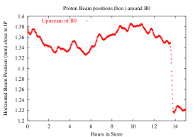
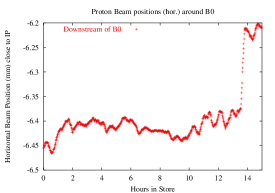
Figure 2: Proton horizontal beam position at BPMs upstream and downstream of CDF. The jump in position coincides with the separator failure

From Figure 2 we observe that just before the failure, the proton horizontal position was relatively steady at 1.349 mm, then it falls for about 15 minutes after which it stabilized at 1.217 mm. Similarly at the downstream BPM, the horizontal positions at these same times are -6.375 mm and -6.214 mm. This slow decay in the position is related to the long integration time (about 15 mins) of these collision point monitors(CPMs).

The observed shifts at the CPMs around CDF were

$${\rm Upstream}:\;\;\;\Delta x_{U}^{obs}=-0.132\;{\rm mm}\;\;\;\;\;\;\;\;\;\;\;\;\;\;\;\;\;\;{\rm Downstream}:\;\;\;\Delta x_{D}^{obs}=0.161\;{\rm mm}$$ (12)

Propagating these orbit shifts to the IP, we find using the upstream BPM that the expected orbit shift at CDF and relative luminosity drops are

$$\Delta x_{co}(CDF)=0.0285\;{\rm mm},\;\;\;\;\;\;\Rightarrow\frac{\Delta{\cal L}}{\cal L}(CDF)=0.384$$ (13)

while using the downstream BPM, we find

$$\Delta x_{co}(CDF)=0.0241\;{\rm mm},\;\;\;\;\;\;\Rightarrow\frac{\Delta{\cal L}}{\cal L}(CDF)=0.293$$ (14)

This calculation shows that the upstream BPM was more consistent with the observed luminosity drop. This may indicate either more errors downstream from the IP to the CPM (this is unlikely since there is only the detector between the IP to the CPM) or that this downstream CPM reading was less reliable.

3 Lifetimes and emittance growth times

The luminosity in terms of beam parameters is

$${\cal L}=\frac{3\gamma f_{rev}M_{b}N_{p}N_{\bar{p}}}{\pi\beta^{*}(\epsilon_{N,p}+\epsilon_{N,\bar{p}})}{\cal H}(\frac{\beta^{*}}{\sigma_{s}})$$ (15)

where $f_{rev}$ is the revolution frequency, $M_{b}$ is the number of bunches in each beam, $N_{p},N_{\bar{p}}$ are the proton and anti-proton bunch intensities respectively, $\epsilon_{N,p},\epsilon_{N,\bar{p}}$ are the 95% emittances of the beams, $\sigma_{s}$ is the rms bunch length and ${\cal H}$ is the hourglass form factor

$${\cal H}(z)=\sqrt{\pi}ze^{z^{2}}(1-\Phi(z)),\;\;\;\;\;\;\;\Phi(z)=\frac{2}{\sqrt{\pi}}\int_{0}^{z}e^{-t^{2}}dt$$ (16)

The average bunch length in Store 1253 was 2.6 nano-seconds or $\sigma_{s}=78$cm. With $\beta^{*}=35$cm, the hourglass reduction factor for $z\equiv\beta^{*}/\sigma_{s}=0.45$ is ${\cal H}(z)=0.51$.

The luminosity lifetime can be calculated from the beam parameters by taking the logarithmic derivatives. Defining the luminosity and intensity lifetimes as

$$\frac{1}{\tau_{\cal L}}=-\frac{1}{\cal L}\frac{d{\cal L}}{dt},\;\;\;\;\;\;\;\;\;\frac{1}{\tau_{p}}=-\frac{1}{N_{p}}\frac{dN_{p}}{dt},\;\;\;\;\;\;\;\frac{1}{\tau_{\bar{p}}}=-\frac{1}{N_{\bar{p}}}\frac{dN_{\bar{p}}}{dt}$$ (17)

while the longitudinal bunch length and transverse emittance growth times are

$$\frac{1}{\tau_{s}}=\frac{1}{\sigma_{s}}\frac{d\sigma_{s}}{dt},\;\;\;\;\;\;\;\;\;\frac{1}{\tau_{\epsilon_{\perp}}}=\frac{1}{\epsilon_{N,p}+\epsilon_{N,\bar{p}}}\frac{d}{dt}(\epsilon_{N,p}+\epsilon_{N,\bar{p}})$$ (18)

Then the luminosity lifetime is

$$\frac{1}{\tau_{\cal L}}=\frac{z}{\cal H}\frac{d{\cal H}}{dz}\frac{1}{\tau_{s}}+\frac{1}{\tau_{p}}+\frac{1}{\tau_{\bar{p}}}+\frac{1}{\tau_{\epsilon_{\perp}}}$$ (19)

Here $z=\beta^{*}/\sigma_{s}$. Using the expression for the hour-glass form factor ${\cal H}$, this can be rewritten as an expression for the emittance growth rate,

$$\frac{1}{\tau_{\epsilon_{\perp}}}=\frac{1}{\tau_{\cal L}}-(1-\frac{2z}{\cal H}+2z^{2})\frac{1}{\tau_{s}}-\frac{1}{\tau_{p}}-\frac{1}{\tau_{\bar{p}}}$$ (20)

We calculate the emittance growth time $\tau_{\epsilon_{\perp}}$ from the measured values of the other time scales. This is useful because at this stage in Run II the synchrotron light monitor was not available, so there was no direct measurement of the transverse emittance growth rate during the store.

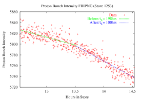
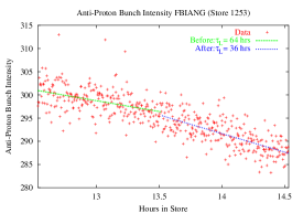
Figure 3: Proton bunch intensity (left) and anti-proton bunch intensity (right) before and after the separator failure. Note the change in slope at around 13.5 hours

Figure 3 shows the proton and anti-proton bunch intensities an hour before and after the separator failure. There is a clear change in the intensity lifetimes before and after the failure.

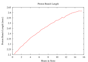
Figure 4: Proton bunch length during the store. The separator failure occurred about at 13.5 hours into the store.

Figure 4 shows the bunch length as a function of time over the store. There is evident growth in the bunch length over the 15 hours of the store but from the data then available (bunch lengths every 15 minutes) it was not possible to discern a change in the growth of the bunch length after the separator failure. We assume that the growth rates of the bunch length were the same an hour before and an hour after the failure. Table 2 shows the measured lifetimes and growth times and the calculated transverse emittance growth time before and after the failure.

	Before separator failure	After separator failure
Luminosity lifetime [hrs]	17	10
Proton lifetime [hrs]	198	100
Anti-proton lifetime [hrs]	64	36
Average Bunch length [nsec]	2.6	2.6
Bunch length growth time [hrs]	81.5	81.5
Transverse Emittance growth time [hrs]	24.5	15.3

Table 2: Lifetimes and growth times from data 1 hour before and an hour after the separator failure. The transverse emittance growth rates are calculated from Equation (3.6).

3.1 Beam lifetime

The separator failure changed the beam orbits around the ring. The changes in the proton orbit were calculated using a MAD optics file. The maximum horizontal orbit change was 1.8$\sigma$ radially outwards while the rms orbit change was 0.59$\sigma$. In the vertical plane, the maximum orbit shift was about 1.8$\sigma$ downwards but the rms orbit change was smaller, 0.24$\sigma$, as expected. An important consequence of the change in orbit is a change in physical aperture. Since the collimators define the limiting aperture, movement towards them would reduce the physical aperture.

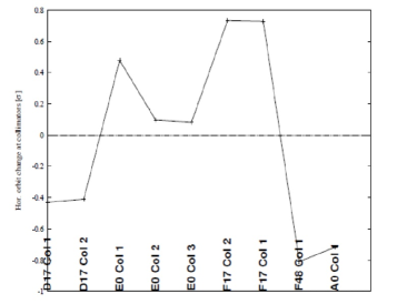
Figure 5: Change in the horizontal proton orbit (in units of the rms beam size) at the collimators due to the separator failure. The largest change was at the F17 collimators where the protons moved by about 0.73 $\sigma$ to the radial outside.

Figure 5 shows the simulated proton horizontal orbit change at several collimators in the ring. The largest change at a collimator location was about 0.73$\sigma$ towards the F17 collimator.

We have seen that the emittance growth rate increased and the orbits changed significantly after the separator failure. Could these two phenomena explain the sharp drop in beam lifetime?

We assume that the beam density distribution function evolves according to the diffusion equation. For simplicity we will consider the transverse distribution function can be decoupled as the product of horizontal $\rho_{x}$ and vertical $\rho_{y}$ distribution functions and consider only the evolution of $\rho_{x}$,

$$\frac{\partial}{\partial t}\rho_{x}=\frac{\partial}{\partial J_{x}}\left[D(J_{x})\frac{\partial\rho_{x}}{\partial J_{x}}\right]$$ (21)

Here $D(J_{x})$ is the diffusion coefficient in the action $J_{x}=[x^{2}+(\beta_{x}x^{\prime}+\alpha_{x})^{2}]/\beta_{x}$. The limiting physical aperture is assumed to be in the horizontal plane at an amplitude $A_{x}$ and corresponding action at the aperture is $J_{A}=A_{x}^{2}/\beta_{x}$. Under the assumption of independence of the transverse planes, the total number of particles in the beam at time $t$ can be written as $N(t)=N_{0}N_{x}(t)N_{y}(t)$ where $N_{0}$ is the initial number of particles, $N_{x}$ is a scaled time dependent number defined by

$$N_{x}(t)=\int_{0}^{J_{A}}\rho_{x}(J_{x},t)\;dJ_{x},\;\;\;N_{x}(0)=1$$ (22)

and a similar expression for $N_{y}$. We assume that particles that diffuse out to the aperture $J_{A}$ are lost.

The beam emittance $\epsilon_{x}$ is related to the average action which is defined as

$$\langle J_{x}\rangle=\int_{0}^{J_{A}}J_{x}\rho_{C}(J_{x},t)\;dJ_{x}$$ (23)

where $\rho_{C}$ is the conditional density which accounts for the particle number changing in time and hence is defined as $\rho_{C}=\rho_{x}/N_{x}$. From the definition it is clear that $\rho_{C}$ is normalized to unity at all times. It follows from the diffusion equation that the average action evolves as

$$\frac{d}{dt}\langle J_{x}\rangle=\int_{0}^{J_{A}}D^{\prime}(J_{x})\rho_{C}\;dJ_{x}+[J_{A}-\langle J_{x}\rangle]D(J_{A})\frac{\partial\rho_{C}}{\partial J_{x}}(J_{A})$$ (24)

If the density falls sufficiently rapidly and the aperture is far enough away from the beam, then $\partial\rho_{C}(J_{A})/\partial J_{x}\rightarrow 0$ and the second term in the above equation can be dropped. With this simplification,

$$\frac{d}{dt}\langle J_{x}\rangle=\int_{0}^{J_{A}}D^{\prime}(J_{x})\rho_{C}\;dJ_{x}$$ (25)

If the diffusion coefficient increases linearly with the action,

$$D(J_{x})=D_{0}J_{x}$$ (26)

then it follows

$$\frac{d}{dt}\langle J_{x}\rangle=D_{0}$$ (27)

The effective transverse emittance calculated from the luminosity was found to increase nearly linearly with time during stores, we may therefore assume that Equation (26) is valid, at least in the core of the beam.

We can now calculate time scales associated with the diffusive motion. The mean escape time for particles to travel to the absorbing boundary at $J_{A}$ is defined as [2]

$$t_{esc}=\int_{0}^{J_{A}}\frac{J_{x}}{D(J_{x})}\;dJ_{x}$$ (28)

Assuming Equation (26), we obtain

$$t_{esc}=\frac{J_{A}}{D_{0}}$$ (29)

This escape time is related to the beam lifetime.

The lifetime can be calculated by a more complete analysis as in Edwards and Syphers [1]. The diffusion equation can be solved analytically when the diffusion coefficient is linear or quadratic in the action. With a linear dependence as assumed above, the density at time $t$ is

$$\rho_{x}(J_{x},t)=\sum_{n}c_{n}J_{0}(\lambda_{n}\sqrt{\frac{J_{x}}{J_{A}}})\exp[-\frac{\lambda_{n}^{2}}{4}\frac{D_{0}t}{J_{A}}]$$ (30)

where

$$c_{n}=\frac{1}{J_{1}^{2}(\lambda_{n})J_{A}}\int_{0}^{J_{A}}\rho_{0}(\frac{J_{x}}{J_{A}})J_{0}(\lambda_{n}\sqrt{\frac{J_{x}}{J_{A}}})\;dJ_{x}$$ (31)

$J_{0},J_{1}$ are the zeroth and first order Bessel functions, the $\lambda_{n}$’s are the $n$’th roots of $J_{0}$ and $\rho_{0}$ is the initial density. For an initially Gaussian distribution in phase space, the distribution in action is an exponential,

$$\rho_{0}(J_{x})=\alpha\exp[-\frac{\alpha J_{x}}{J_{A}}]\;,\;\;\;\;\;\;\alpha=\frac{A^{2}}{2\sigma_{x}^{2}}$$ (32)

Assuming that the beam is sufficiently far from the aperture, the coefficients $c_{n}$ simplify in this case to

$$c_{n}=\frac{1}{J_{1}^{2}(\lambda_{n})}\exp[-\frac{\lambda_{n}^{2}}{4\alpha}]$$ (33)

Keeping only the first and dominant term in the solution for the density Equation (30), the scaled partial number of particles $N_{x}$ in the beam simplifies to

$$N_{x}(t)\simeq\frac{2}{\lambda_{1}J_{1}(\lambda_{1})}\exp[-\frac{\lambda_{1}^{2}}{2}(\frac{\sigma_{x}}{A})^{2}]\exp[-\frac{\lambda_{1}^{2}}{4}\frac{D_{0}t}{J_{A}}]$$ (34)

We assume that the lifetime was determined by particles reaching the horizontal aperture first. It follows that the lifetime defined as

$$t_{L}=-\frac{N_{x}}{dN_{x}/dt}=\frac{4}{\lambda_{1}^{2}}\frac{J_{A}}{D_{0}}\simeq 0.7\frac{J_{A}}{D_{0}}$$ (35)

This expression is very close to the mean escape time $t_{esc}$ calculated in Equation (29).

We will now use Equation (35) to relate the beam lifetimes before and after the separator failure. Equating

$$D_{0}\equiv\frac{d\epsilon_{x}}{dt}=\frac{\epsilon_{0}}{\tau_{\epsilon}}$$ (36)

where $\epsilon_{0}$ is the initial emittance and $\tau_{\epsilon}$ is the emittance growth time. Then

$$t_{L}=0.7\frac{J_{A}}{\epsilon_{0}}\tau_{\epsilon}$$ (37)

Before the separator failure, the beam aperture was approximately $6\sigma$ at one or more of the collimators. Hence before the failure, $J_{A}=(6\sigma)^{2}/\beta_{x}$. After the failure the beam moved closer to the physical aperture by 0.7$\sigma$. Hence $J_{A}=(5.3\sigma)^{2}/\beta_{x}$ after the failure.

$$\Rightarrow\frac{t_{L}({\rm after})}{t_{L}({\rm before})}=\frac{J_{A}({\rm after})}{J_{A}({\rm before})}\frac{\tau_{\epsilon}({\rm after})}{\tau_{\epsilon}({\rm before})}$$ (38)

From Table 2 we find that $\tau_{\epsilon}({\rm before})=24.5$hrs and $\tau_{\epsilon}({\rm after})=15.3$hrs. Hence

$$\frac{t_{L}({\rm after})}{t_{L}({\rm before})}=(\frac{5.3}{6})^{2}\frac{15.3}{24.5}=0.49$$ (39)

From Table 2 we find that the ratio of the measured lifetimes is $=100/198=0.51$. Hence the predictions of the one dimensional theory are in very good agreement with the observed drop in lifetime. The increased emittance growth after the separator failure may have been due to multiple sources resulting from the change in orbits including change in tunes, increased long-range beam-beam effects from smaller separations at some locations and larger nonlinear fields in some magnets etc.

No matter what the sources of emittance growth were, we have shown that the drop in lifetime after the separator failure was consistent with a simple model of diffusive emittance growth and the beam center moving closer to a physical aperture.

References

- [1] D. Edwards and M.J. Syphers,An Introduction to the Physics of High Energy Accelerators, John Wiley (1993)
- [2] C.W. Gardiner,Handbook of Stochastic Methods, Springer-Verlag (1985)