Percolation in phase transition Critical phenomena in thermodynamics Stochastic process

Percolation Theory on Interdependent Networks
Based on Epidemic Spreading

Abstract

We consider percolation on interdependent locally treelike networks, recently introduced by Buldyrev et al., Nature 464, 1025 (2010), and demonstrate that the problem can be simplified conceptually by deleting all references to cascades of failures. Such cascades do exist, but their explicit treatment just complicates the theory – which is a straightforward extension of the usual epidemic spreading theory on a single network. Our method has the added benefits that it is directly formulated in terms of an order parameter and its modular structure can be easily extended to other problems, e.g. to any number of interdependent networks, or to networks with dependency links.

On September 28, 2003, Italy experienced its most severe blackout in over 20 years [1]. The blackout’s severity was later attributed to the fact that an initial failure on the physical power grid disrupted not only the grid, itself, but also a computer network that depended on this grid for electricity [1, 2]. Since the grid’s substations were, in turn, dependent on this computer network for their regulation, further failures in the grid ensued as communication among the stations was lost. Ultimately, recursive cascading failures throughout both networks occurred, and both networks changed from percolating to non-percolating [1, 2, 3, 4]. While this is a spectacular example of percolation on interdependent networks, it is, by no means the only one: in fact, most real-world networks can be seen as having some interdependency [5, 6, 7]. A clear description of how perturbations propagate through such networks – i.e. of how perturbations can effect percolation (fragmentation) – is essential to understanding systems involving interdependence, including economic markets, interrelated technological and infrastructural systems, social networks, disease dynamics, or human physiology.

Recent models of percolation on interdependent networks have been described in terms of failures cascading back and forth between the networks  [2, 3, 4]. While there is no doubt that percolation on interdependent networks can be seen as a cascading phenomenon, the mathematics behind such a description is cumbersome and far from transparent. Here we simplify matters by omitting all aspects of cascading and treat percolation on interdependent networks as an epidemic spreading process in complete analogy to ordinary percolation. If one wants to consider cascades explicitly, this can be done in a second step, after the phase transition itself is well understood. We also show that percolation on dependency networks [4, 8], which are single networks composed of both connectivity links and dependency links, can be described within the same paradigm.

Both the theory of [2, 3, 4] and the present paper deal only with locally treelike random networks, for which mean field theory based on generating functions becomes exact in the large system limit. The cascade-based studies in [2, 3, 4] considered site percolation networks from which a certain fraction $1-p$ of nodes had been removed. On general networks (including lattices), this site dilution can lead to a topological modification of the networks [9], but in the present cases it just leads to a trivial rescaling of the number of nodes and links. Thus we can restrict ourselves, without loss of generality, to the case $p=1$ and only consider bond percolation, which further simplifies the discussion.

In the following, we first recall the theory of epidemic spreading (ordinary percolation theory) on single networks [10, 11], and then demonstrate how this can be easily adjusted to accommodate percolation on interdependent networks or on dependency networks. We only consider the limit of large networks, where the number of nodes $N\to\infty$.

(i) Single network - First consider a single (isolated) random network with mean degree $z$, with an epidemic spreading from some starting node. Let $S_{i}$ be the probability that node $i$ is infected during this epidemic (i.e. that it is part of the infinite percolating cluster). Its average over all nodes, denoted as $S$, is taken as the order parameter of the model. The probability that node $i$ is not infected is equal to the chance that none of its neighbors are infected through their remaining links:

$$1-S_{i}=\prod_{\langle ij\rangle}(1-S^{\prime}_{j}),$$ (1)

where the product runs over all neighbors of $i$ and $S^{\prime}_{j}$ is the probability that node $j$ is infected through a randomly chosen edge not attached to $i$. When the graph is locally treelike, all $S^{\prime}_{j}$ are independent. Averaging Eq. (1) over all nodes gives then

$$S=1-\sum_{k}p(k)(1-S^{\prime})^{k}\equiv 1-G_{0}(1-S^{\prime}),$$ (2)

where $p(k)$ is the probability that a node has $k$ links and $G_{0}(x)$ is the corresponding generating function $G_{0}(x)\equiv\sum_{k}p(k)x^{k}$. Similarly, one can write down the equation for $S^{\prime}$

$$S^{\prime}=1-\sum_{k}{kp(k)\over z}(1-S^{\prime})^{k-1}\equiv 1-G_{1}(1-S^{\prime}),$$ (3)

where $z=G^{\prime}_{0}(1)$ and $G_{1}(x)\equiv G^{\prime}_{0}(x)/z$. For any given degree distribution we can first solve Eq. (3) to obtain $S^{\prime}$, and then insert it into Eq. (2) to obtain $S$. The percolation transition threshold $z_{c}$ is given by $S=0$ for $z<z_{c}$ and $S>0$ for $z>z_{c}$ [10, 11].

For instance, the degree distribution of Erdös-Rényi (ER) graphs [12, 11] is Poissonian. Therefore,

$$G_{0}(1-S^{\prime}) = \sum_{k}{e^{-z}z^{k}\over k!}(1-S^{\prime})^{k}=e^{-zS^{\prime}}$$ (4)

$$= G_{1}(1-S^{\prime}).$$

Thus, $S=S^{\prime}$ and Eqs. (2) and (3) give simply $S=1-e^{-zS}$. Defining $f(S)=S-1+{e}^{-zS}$, one can find the solution $S(z)$ by solving $f(S)=0$ graphically, as shown in Fig. 1. A continuous (‘second order’) phase transition is clearly evident in the inset of Fig. 1.

Figure 1: Graphical solutions for ordinary percolation on a single ER network. The inset shows the continuous change of order parameter $S$ as $z$ increases.

Equations (2) and (3), are the order parameters for a single network, where $S$ represents the probability that a randomly chosen node places in the infinite percolating cluster and $S^{\prime}$ is the same probability, but defined when we pick an edge randomly and look at the end node. These equations act as fundamental ‘building blocks’ or ‘modules’ for treating analogously the probability, on fully or partially interdependent networks, to be connected to the infinite percolating clusters.

(ii) Two fully interdependent networks - Consider now two networks $\cal{A}$ and $\cal{B}$, where each node in ${\cal A}$ depends only on one node in ${\cal B}$ and vice versa. In order for a node in network ${\cal A}$ to be part of the percolating cluster, its partner in ${\cal B}$ must also be part of that cluster. Since this mapping is one-to-one we can merge each node in ${\cal A}$ with its partner in ${\cal B}$ to have one set of nodes, each with two sets of links. We define $\cal{AB}$-clusters as subsets of nodes connected both in $\cal{A}$ and in $\cal{B}$. More precisely a set of nodes $C=\{i_{1},i_{2},\ldots i_{m}\}$ is an $\cal{AB}$-cluster if any two points $i,j\in C$ are connected by two paths: one path using only links $\in\cal{A}$ and nodes only $\in C$, and the other using only links $\in\cal{B}$ and also using nodes only $\in C$. We do not allow paths that involve nodes outside $C$, so $\cal{AB}$-clusters are self-sustaining [9].

The probability that any node belongs to the infinite $\cal{AB}$-cluster is equal to the probability to be linked to it both via $\cal{A}$- and via $\cal{B}$-links. That is, a node looks out at its ${\cal A}$-links to see if it has a neighbor on the percolating ${\cal AB}$-cluster. It also looks out via its ${\cal B}$ links. Only if it has a neighbor via both sets of links is it a member of this cluster. Therefore $S$ is simply a product of the right hand side of Eq. (2) for networks ${\cal A}$ and ${\cal B}$,

$$S=(1-G^{\cal{A}}_{0}(1-S^{\prime}_{\cal{A}}))(1-G^{\cal{B}}_{0}(1-S^{\prime}_{\cal{B}})),$$ (5)

where the superscripts (subscripts) $\cal{A}$ and $\cal{B}$ refer to networks $\cal{A}$ and $\cal{B}$ respectively and $S_{\cal{A}}=S_{\cal{B}}=S$. Here, $S^{\prime}_{\cal{A}}$ (and analogously $S^{\prime}_{\cal{B}}$) is defined as the probability that a node reached by following a random $\cal{A}$-link is in the ${\cal AB}$-cluster. For this to happen, its partner node – which is a random node from the point of view of network $\cal{B}$ – has also to be connected to the ${\cal AB}$-cluster via $\cal{B}$-links. $S^{\prime}_{\cal{A}}$ and $S^{\prime}_{\cal{B}}$ are different from each other since they depend on the degree distribution of each network. When choosing edges at random, the end node of a randomly chosen edge in network $\cal{A}$ belongs to the $\cal{AB}$-cluster only when its partner node in network $\cal{B}$ is concurrently a member of this cluster, and vice versa. The probabilities of these events occurring – $S^{\prime}_{\cal{A}}$ and $S^{\prime}_{\cal{B}}$ – are given by

$$S^{\prime}_{\cal{A}} = (1-G^{\cal{A}}_{1}(1-S^{\prime}_{\cal{A}}))(1-G^{\cal{B}}_{0}(1-S^{\prime}_{\cal{B}})),$$

$$S^{\prime}_{\cal{B}} = (1-G^{\cal{B}}_{1}(1-S^{\prime}_{\cal{B}}))(1-G^{\cal{A}}_{0}(1-S^{\prime}_{\cal{A}})).$$ (6)

Figure 2: Graphical solutions for the percolating cluster on two fully coupled ER networks with the same mean degree $z$. The inset shows a discontinuous change of order parameter $S$ as $z$ increases.

Using this and Eq. (4) for two interdependent ER networks with mean degrees $z_{\cal{A}}$ and $z_{\cal{B}}$ gives

$$S=(1-e^{-z_{\cal A}S})(1-e^{-z_{\cal B}S}).$$ (7)

In particular, when $z_{\cal{A}}=z_{\cal{B}}=z$, the order parameter obeys

$$S=(1-e^{-zS})^{2}.$$ (8)

Defining $g(S)=S-(1-e^{-zS})^{2}$, one can find graphically the value of $S$ as a function of $z$ that solves $g(S)=0$ (see Fig. 2). This solution shows a discontinuous (‘first order’) phase transition (inset of Fig. 2), contrary to the result for the single network in Fig. 1. Demanding $g(S)=g^{\prime}(S)=0$ we find a critical point $S_{c}=0.511699\cdots$ and $z_{c}=2.455407\cdots$. The value of $z_{c}$ agrees with that given for ER networks in [2, 9] and our explicitly determined value of the order parameter just above the critical point, $S_{c}$, can also be obtained from appropriate combinations of their results.

For the general case $z_{\cal{A}}\neq z_{\cal{B}}$, defining

$$h(S)=S-(1-e^{-z_{\cal A}S})(1-e^{-z_{\cal B}S}),$$ (9)

we obtain a line of discontinuous transition points from the conditions $h(S)=0$ and $h^{\prime}(S)=0$. Assuming $h(S)=0$, the second condition can be written as

$$h^{\prime}(S) = 1-z_{\cal A}e^{-z_{\cal A}S}(1-e^{-z_{\cal B}S})-z_{\cal B}e^{-z_{\cal B}S}(1-e^{-z_{\cal A}S})$$ (10)

$$= 1-{{z_{\cal A}S~{}e^{-z_{\cal A}S}}\over{1-e^{-z_{\cal A}S}}}-{{z_{\cal B}S~{}e^{-z_{\cal B}S}}\over{1-e^{-z_{\cal B}S}}}$$

$$= 1-{{x}\over{e^{x}-1}}-{{y}\over{e^{y}-1}}=0,$$

where $x=z_{\cal A}S$ and $y=z_{\cal B}S$. This gives a one-parameter set of solutions $y(x)$, from which $S_{c}$ can be obtained using Eq. (7). Finally, $z_{\cal A}$ and $z_{\cal B}$ are obtained by $z_{\cal A}=x/S$ and $z_{\cal B}=y/S$. The resulting discontinuous phase transition line is shown in Fig. 3(b), where $z_{\cal A}=1$ and $z_{\cal B}=1$ act as asymptotes. In the inset of Fig. 3(b), the jump size $S_{c}$ is shown as a function of the ratio $z_{\cal A}/z_{\cal B}$ (only $z_{\cal A}/z_{\cal B}<1$ is shown, since the transition line is symmetric about the line $z_{\cal A}=z_{\cal B}$). The full dependence of $S$ on $z_{\cal A}$ and $z_{\cal B}$ is shown in Fig. 3(a).

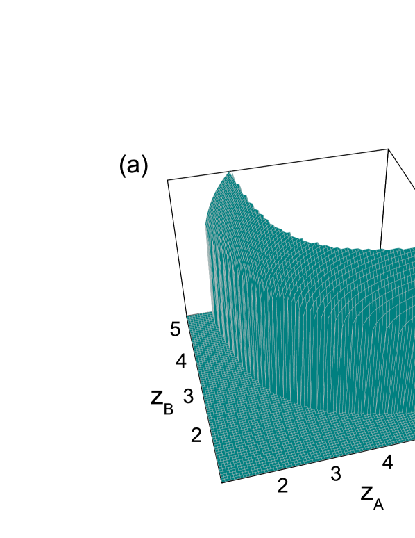
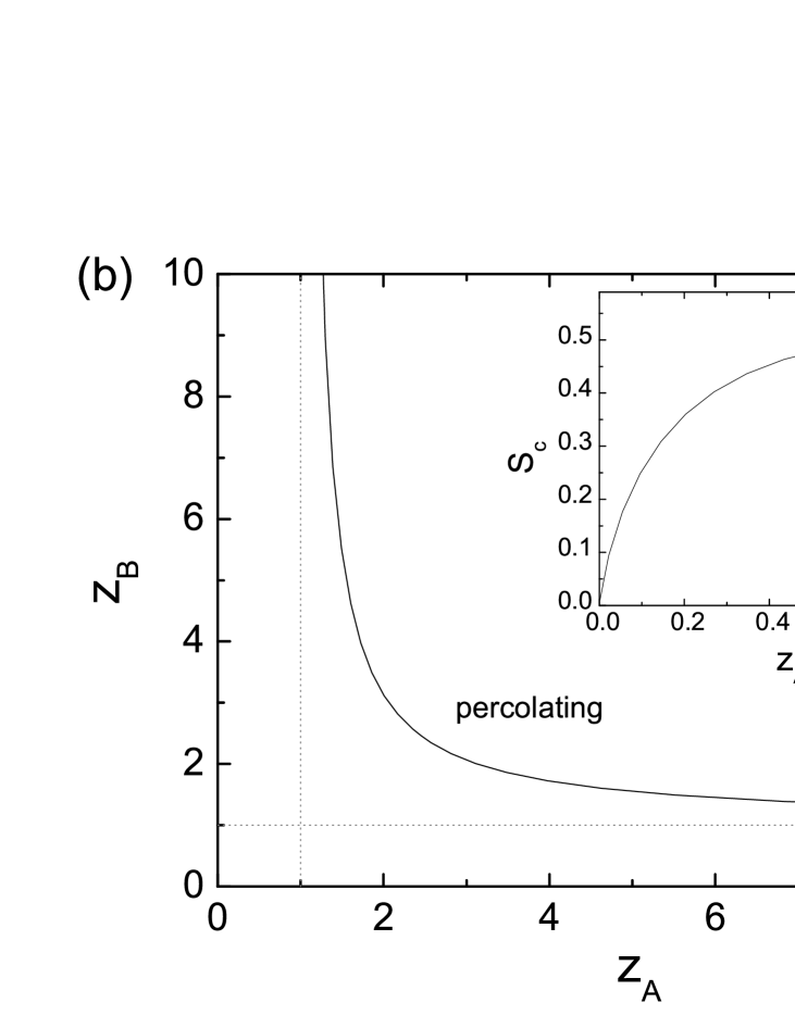
Figure 3: (a) $S$ as a function of $z_{\cal A}$ and $z_{\cal B}$ for Eq. (7). (b) The discontinuous phase transition line on the plane of $z_{\cal A}$ and $z_{\cal B}$. It is symmetric about the line $z_{\cal A}=z_{\cal B}$. In the inset, the jump size $S_{c}$ at the transition line is shown as a function of the ratio $z_{\cal A}/z_{\cal B}$.

(iii) An arbitrary number of interdependent networks - Our approach is easily extended to treat coupling of more than two networks [13]. For $M$ networks, Eqs. (5) and (6) can be simply replaced by

$$S = \prod_{m=1}^{M}(1-{G^{m}_{0}(1-S^{\prime}_{m})}),$$

$$S^{\prime}_{m} = \frac{1-{G^{m}_{1}(1-S^{\prime}_{m})}}{1-{G^{m}_{0}(1-S^{\prime}_{m})}}~{}S.~{}$$ (11)

This is due to the fact that in order to be part of the infinite percolating cluster each node must, by definition, be connected to it via all of the $M$ networks. Order parameters and transition points can be obtained in an analogous way and the transition is discontinuous for any $M>1$.

(iv) Partially interdependent networks - Assume now that two networks are not totally interdependent. In network $\cal{A}$ only a fraction $q_{\cal{A}}$ of the nodes are dependent on a node in network $\cal{B}$. To be on the percolating cluster, a node has to be connected to the cluster via ${\cal A}$ links and the node on which it depends has to be connected to the cluster via ${\cal B}$ links. Similarly a fraction $q_{\cal B}$ of nodes in network $\cal{B}$ depend on a node in $\cal{A}$. Note that here one node from a network depends only on one node from the other network, i.e., each node can have only one dependency link, which can be unidirectional or bidirectional [3]. In that case, in general we must expect that the two order parameters $S_{\cal{A}}$ and $S_{\cal{B}}$ are different. They indicate the chance that a randomly picked node in $\cal{A}$ (resp. $\cal{B}$) is a member of the percolating $\cal{AB}$-cluster.

Let us first discuss the symmetric case $q_{\cal{A}}=q_{\cal{B}}=q$. If a given node in network $\cal{A}$ does not depend on network $\cal{B}$ (which happens with probability $1-q$), it is a member of the percolating ${\cal AB}$-cluster iff at least one of its neighbors in $\cal{A}$ is also a member of that cluster. On the other hand, with probability $q$, the node does depend on a node in $\cal{B}$. In that case, in order for it to be part of the percolating ${\cal AB}$-cluster, its dependency partner also must be connected via network $\cal{B}$ to at least one node in that cluster. Therefore, the probability $S_{\cal{A}}$ can be expressed by summing the conditional probability to be connected multiplied by the corresponding probability to be dependent ($q$) or not ($1-q$):

$$S_{\cal{A}} = q(1-G^{\cal{A}}_{0}(1-S^{\prime}_{\cal{A}}))(1-G^{\cal{B}}_{0}(1-S^{\prime}_{\cal{B}}))$$ (12)

$$+(1-q)(1-G^{\cal{A}}_{0}(1-S^{\prime}_{\cal{A}}))$$

$$= (1-G^{\cal{A}}_{0}(1-S^{\prime}_{\cal{A}}))(1-qG^{\cal{B}}_{0}(1-S^{\prime}_{\cal{B}})).~{}$$

Similarly,

$$S^{\prime}_{\cal{A}}=(1-G^{\cal{A}}_{1}(1-S^{\prime}_{\cal{A}}))(1-qG^{\cal{B}}_{0}(1-S^{\prime}_{\cal{B}})).~{}$$ (13)

By symmetry, another pair of conditions exists for network $\cal{B}$:

$$S_{\cal{B}} = (1-G^{\cal{B}}_{0}(1-S^{\prime}_{\cal{B}}))(1-qG^{\cal{A}}_{0}(1-S^{\prime}_{\cal{A}})),$$

$$S^{\prime}_{\cal{B}} = (1-G^{\cal{B}}_{1}(1-S^{\prime}_{\cal{B}}))(1-qG^{\cal{A}}_{0}(1-S^{\prime}_{\cal{A}})).$$ (14)

More generally, if $q_{\cal{A}}\neq q_{\cal{B}}$,

$$S_{\cal{A}} = (1-G^{\cal{A}}_{0}(1-S^{\prime}_{\cal{A}}))(1-q_{\cal{A}}G^{\cal{B}}_{0}(1-S^{\prime}_{\cal{B}})),$$

$$S^{\prime}_{\cal{A}} = (1-G^{\cal{A}}_{1}(1-S^{\prime}_{\cal{A}}))(1-q_{\cal{A}}G^{\cal{B}}_{0}(1-S^{\prime}_{\cal{B}})),$$

$$S_{\cal{B}} = (1-G^{\cal{B}}_{0}(1-S^{\prime}_{\cal{B}}))(1-q_{\cal{B}}G^{\cal{A}}_{0}(1-S^{\prime}_{\cal{A}})),$$

$$S^{\prime}_{\cal{B}} = (1-G^{\cal{B}}_{1}(1-S^{\prime}_{\cal{B}}))(1-q_{\cal{B}}G^{\cal{A}}_{0}(1-S^{\prime}_{\cal{A}})).$$ (15)

Again, these four coupled equations involve nothing more complicated than (weighted) products of the network-specific fundamental factors from Eqs. (2) and (3). Together, they give the behavior of the order parameters $S_{\cal{A}}$ and $S_{\cal{B}}$. These expressions are completely equivalent to the more complicated results in [3]. If $q_{\cal{A}}=q_{\cal{B}}=q=1$, these equations reduce to Eqs. (5) and (6).

If $q_{\cal{A}}=q_{\cal{B}}=q\neq 1$ and if the two networks have the same degree distribution, $S_{\cal{A}}=S_{\cal{B}}=S$. For example, if two ER networks having the same mean degree $z$ are coupled with the dependency probability $q\neq 1$, the solution is simply

$$S=(1-e^{-zS})(1-qe^{-zS}).$$ (16)

The solution $S$ can now be expressed as a function of both $z$ and $q$. When $q=0$, $S(z)$ shows a continuous transition, since now both networks are fully independent. On the other hand, when $q=1$, the transition is discontinuous. A crossover from second order behavior to first order behavior at the tricritical point $q_{c}$ is observed as $q$ is increased from 0 to 1. In analogy to Eq. (9), we now define

$$h(S)=S-(1-e^{-zS})(1-qe^{-zS}),$$ (17)

The tricritical point is found by demanding $S=h(S)=h^{\prime}(S)=h^{\prime\prime}(S)=0$, which gives $q_{c}=1/3$ and $z_{c}=3/2$ [3].

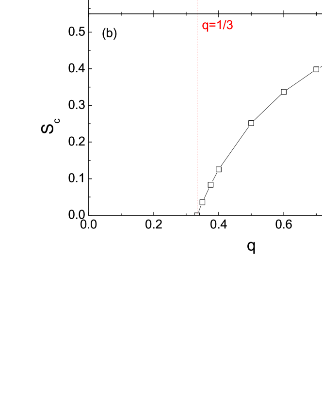
Figure 4: (Color online) (a) Percolation transition points for two partially coupled ER networks with the same mean degree $z$ at different values of the dependency $q$. (b) The jump size $S_{c}$ at the transition point. The first order phase transition line ($q>1/3$) meets the second order phase transition line ($q<1/3$) at $q=1/3$. The red dotted line indicates the tricritical point $(q_{c},z_{c})=(1/3,3/2)$.

For $q>q_{c}$, we can find the first order transition point by considering $h(S)=0$ and $h^{\prime}(S)=0$. The subsequent analysis is straightforward and follows closely our previous method. Its results are displayed in Fig. 4.

Let us briefly discuss the case $q_{\cal{A}}=q_{\cal{B}}=q$ and $z_{\cal{A}}\neq z_{\cal{B}}$ of ER networks, which was not treated before. In this case, also $S_{\cal{A}}\neq S_{\cal{B}}$, and we have to solve the coupled equations

$$h_{\cal{A}}(S_{\cal{A}})=S_{\cal{A}}-(1-e^{-z_{\cal{A}}S_{\cal{A}}})(1-qe^{-z_{\cal{B}}S_{\cal{B}}})=0,$$ (18)

$$h_{\cal{B}}(S_{\cal{B}})=S_{\cal{B}}-(1-e^{-z_{\cal{B}}S_{\cal{B}}})(1-qe^{-z_{\cal{A}}S_{\cal{A}}})=0.$$

The percolation transition is obtained by imposing in addition $h^{\prime}_{\cal{A}}(S_{\cal{A}})=h^{\prime}_{\cal{B}}(S_{\cal{B}})=0$. Defining again $x=z_{\cal{A}}S_{\cal{A}}$ and $y=z_{\cal{B}}S_{\cal{B}}$, we find

$$\left(1-{{x}\over{e^{x}-1}}\right)\left(1-{{y}\over{e^{y}-1}}\right)={{qx}\over{e^{x}-q}}\times{{qy}\over{e^{y}-q}}~{}~{}.$$ (19)

For given $q$ this is solved graphically (Fig. 5). The values of $S_{\cal{A}}$ and $S_{\cal{B}}$ at the transition point are then obtained from Eq. (18). If they vanish, the transition is continuous, otherwise it is discontinuous. Results are shown in Fig. 5 for $q=1/2$. If $q$ decreases, the two tricritical points move together. They coalesce at $z_{\cal{A}}=z_{\cal{B}}=3/2$ when $q\to 1/3$.

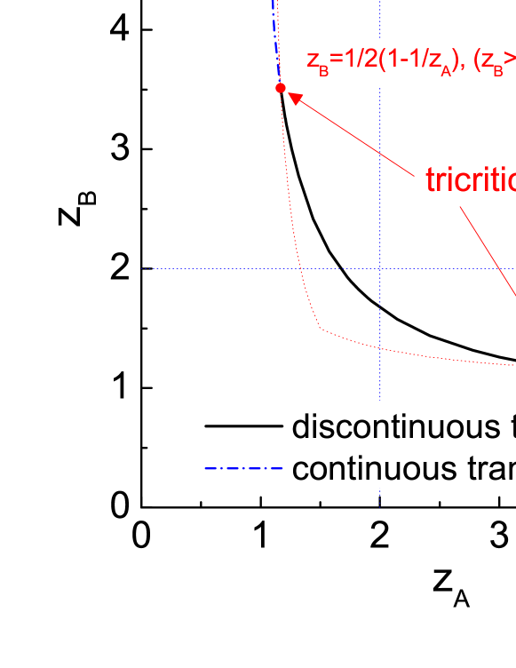
Figure 5: (Color online) Phase transition line at $q=1/2$ for different $z_{\cal{A}}$ and $z_{\cal{B}}$. The black solid line indicates the first order transition line and the blue dash-dot line represents the second order transitions. They meet two tricritical points (red bullets). The tricritical points move along the red dotted line as $q$ changes. When $q=1/3$, the tricritical points meet at $z_{\cal{A}}=z_{\cal{B}}=3/2$.

(v) Dependency networks - A dependency network [4, 8] is a single network that contains two types of links, connectivity links and dependency links. In the simplest case each node in the network depends on one other node in that network and all dependencies are mutual. In order for a node to be connected to the infinite self-sustaining cluster both it and its partner must be part of that cluster. For random networks this leads immediately to Eqs. (5) and (6) where the subscripts ${\cal A}$ and ${\cal B}$ are dropped since there is only one network. In the case that only a fraction $q$ of nodes have dependency links we get Eqs. (12) and (13), again dropping the subscripts labelling the networks. Again the type of transition depends on the value of $q$, with a tricritical point separating the two regimes.

In the most general case where a node has $m$ dependency links with probability $p(m)$ the resulting equations are

$$S=\sum_{m=0}^{N-1}p(m)(1-G_{0}(1-S^{\prime}))^{m+1},$$

$$S^{\prime}=(1-G_{1}(1-S^{\prime}))\sum_{m=0}^{N-1}p(m)(1-G_{0}(1-S^{\prime}))^{m}.$$

Again the precise behavior reflects the extent to which the network is dependent, with a low dependency regime exhibiting a continuous transition in the universality class of ordinary percolation and a high dependency regime exhibiting a first order transition, with crossover controlled by a tricritical point. Similar arguments can be used to derive the general case for interdependent networks where a single node has dependencies to $m$ other networks with probability $p(m)$. In that case the equations are more complicated because each network’s structure may be different and they will have different order parameters, but the arguments used to derive the equations are precisely the same. The above does not apply to networks with directed (non-mutual) dependencies, for which different arguments apply.

In summary, we consider percolation on various interdependent or dependency networks, pointing out the close analogy to epidemic spreading on single networks without these dependencies. Our arguments are much more straightforward, both conceptually and mathematically, than previous ones built on cascades of failures. We should however stress that they apply, like those of [2, 3, 4, 13, 8] only to random locally treelike graphs. For interdependent networks that are correlated with each other [14] or that are spatially embedded [9, 15] the transition is in general not first order, and the interdependency can make the transition even less sharp than in ordinary percolation [9, 15]. For these more realistic cases no analytical theory is yet available.

References

- [1] V. Rosato, et al., Int. J. Crit. Infrastruct. 4, 63 (2008).
- [2] S. V. Buldyrev, R. Parshani, G. Paul, H. E. Stanley, and S. Havlin, Nature 464, 1025 (2010).
- [3] R. Parshani, S. V. Buldyrev, and S. Havlin, Phys. Rev. Lett. 105, 048701 (2010).
- [4] R. Parshani, S. V. Buldyrev, and S. Havlin, Proc. Natl. Acad. Sci. USA 108, 1007 (2011).
- [5] Y. Moreno, R. Pastor-Satorras, A. Vázquez, and A. Vespignani, Europhys. Lett. 62, 292 (2003).
- [6] A. E. Motter, Phys. Rev. Lett. 93, 098701 (2004).
- [7] M. Kurant and P. Thiran, Phys. Rev. Lett. 96, 138701 (2006).
- [8] A. Bashan and S. Havlin, arXiv:1106.1631 (2011).
- [9] S.-W. Son, P. Grassberger, and M. Paczuski, arXiv:1108.3863 (2011).
- [10] M. E. J. Newman, Phys. Rev. Lett. 95, 108701 (2005).
- [11] M. E. J. Newman, S. H. Strogatz, and D. J. Watts, Phys. Rev. E 64, 026118 (2001).
- [12] B. Bollobás, Random Graphs (Academic Press, London, 1985).
- [13] J. Gao, S.V. Buldyrev, S. Havlin, and H.E. Stanley, arXiv:1010.5829 (2010).
- [14] R. Parshani, C. Rozenblat, D. Ietri, C. Ducruet, and S. Havlin, arXiv:1010.4506 (2010).
- [15] S.-W. Son P. Grassberger, and M. Paczuski, to be published.