Temperature dependent compressibility in graphene and 2D systems

Abstract

We calculate the finite temperature compressibility for two-dimensional semiconductor systems, monolayer graphene, and bilayer graphene within the Hartree-Fock approximation. We find that the calculated temperature dependent compressibility including exchange energy is non-monotonic. In 2D systems at low temperatures the inverse compressibility decreases first with increasing temperature, but after reaching a minimum it increases as temperature is raised further. At high enough temperatures the negative compressibility of low density systems induced by the exchange energy becomes positive due to the dominance of the finite temperature kinetic energy. The inverse compressibility in monolayer graphene is always positive and its temperature dependence appears to be reverse of the 2D semiconductor systems, i.e., it increases first with temperature and then decreases at high temperatures. The inverse compressibility of bilayer graphene shows the same non-monotonic behavior as ordinary 2D systems, but at high temperatures it approaches a constant which is smaller than the value of the non-interacting bilayer graphene. We find the leading order temperature correction to the compressibility within Hartree-Fock approximation to be $T^{2}\ln T$ at low temperatures for all three systems.

I Introduction

In this article, we provide a detailed theory for the temperature-dependent electronic compressibility ($K$) of an interacting two dimensional (2D) electron (or hole) system within the Hartree-Fock theory. We consider three distinct 2D systems of active current interest in condensed matter physics: 2D semiconductor systems (e.g., quantum wells, heterostructures, inversion layers, etc.); monolayer graphene; bilayer graphene. For the purpose of comparison (and also for the sake of completeness), we also provide as an appendix the corresponding finite temperature Hartree-Fock compressibility for a standard three dimensional electron gas (3DEG) since this result does not appear to be available in the theoretical literature in spite of the sixty-year long history of studying many-body interaction effects in 3DEG.

Ever since the pioneering measurement of the 2D compressibility by Eisenstein et al., Eisenstein et al. (1992, 1994) it has been extensively studied in 2D systems because the compressibility provides fundamental insight into quantum ground state properties which are not readily obtained from transport measurements. Some experimental studies Dultz and Jiang (2000); Ilani et al. (2000); Dultz et al. of the compressibility have shed light on understanding the 2D metal-insulator transition (MIT)Das Sarma and Hwang (2005). The inverse compressibility ($K^{-1}$) is positive when the kinetic energy dominates over interactions at high densities. As the 2D density is reduced $K^{-1}$ changes sign and becomes negative due to the increase of exchange energy associated with electron-electron interactionEisenstein et al. (1992, 1994). The negative $K^{-1}$ reaches a minimum value at a certain low density $n$, and then increases dramatically with further decreasing $n$ as the 2D MIT sets in. The minimum point in $K^{-1}$ has occasionally been loosely identified as the critical density for the 2D MIT and is closely related to the transition from a homogeneous system to an inhomogeneous nonlinear screening regime, Ilani et al. (2000); Shi and Xie (2002) where the system is dominated by the formation of electron (or hole) puddles. Whether this observed low-density behavior of $K$ is a cause for or an effect of 2D MIT is unclear. The low-density compressibility of 2D electronic (in this paper we use the term “electron” to imply either electron or hole as should be obvious from the context) systems has been of interest for almost 20 years now with the early experimentsEisenstein et al. (1992, 1994); Dultz and Jiang (2000); Ilani et al. (2000); Dultz et al. studying semiconductor-based 2D systems extensively and very recent experiments studying monolayer and bilayer graphene. The reason for the focus on the density dependence of compressibility is that, in general, quantum interaction effects increase monotonically with decreasing density in a Coulomb system (with monolayer graphene being an odd exception where the interaction parameter, the so-called graphene fine structure constant, is independent of carrier densityDas Sarma et al. (2011)), as discussed above, leading eventually to the electronic compressibility becoming negative at low, but easily accessible, densities due to exchange effects.

It is curious, however, that in spite of this intense interest in the strongly interacting low-density 2D compressibility, there has been little research on the theoretical functional dependence of 2D compressibility on temperature. This is strange because the scale for the temperature dependence of any electronic property is the Fermi temperature $T_{F}=E_{F}/k_{B}$, which invariably decreases with decreasing density. Thus, temperature effects on 2D compressibility become progressively more important even at a fixed temperature as the electron density goes down, since the important dimensionless temperature $t\equiv T/T_{F}$ increases with decreasing density even if $T$ is kept fixed. For example, 2D GaAs holes have $T_{F}<1$ K for a hole density of $10^{10}$ cm^-2, which means that $T=1$ K is effectively a high-temperature regime for 2D hole densities $\lesssim 10^{10}$ cm^-2! Our work in this paper takes a first step in correcting this omission in the literature. Our results are important for interpreting low-density 2D compressibility (even at relatively low temperatures) existing in the literature.

The thermodynamic isothermal compressibility (or simply compressibility) of a system is defined as the change of pressure with volume, $K=-V^{-1}(\partial V/\partial P)_{N,T}$, where $N$ is the particle number, $T$ is the temperature, $V$ is the system volume, $P=-(\partial E/\partial V)_{N,T}$ is the pressure, and $E$ is the total energy of the system. Thus, $K^{-1}\equiv V(\partial^{2}E/\partial V^{2})$. In the non-degenerate or classical systems the velocity of thermodynamic sound, $v_{0}$, often provides a convenient experimental measure of compressibility, $v_{0}^{2}=\frac{1}{mn}\frac{1}{K}$, where $m$ and $n=N/V$ are the mass and the density of the system, respectively. In the quantum limit the compressibility can be obtained theoretically by using the theorem of Seitz Pines and Nozieres (1966), (i.e., by connecting $K$ with the change in chemical potential with density, $\partial\mu/\partial n$, where $\mu$ is the chemical potential and $n$ is the carrier density of the system). Another method of evaluating $K$ is through the compressibility sum rule. This is an exact relationship between the compressibility and the long wavelength limit of the static dielectric function Mahan (2000). In 2D quantum systems the compressibility is often measured from the quantum capacitance Eisenstein et al. (1992, 1994) which is proportional to $dn/d\mu\propto K$. A scanning single electron transistor has also been used to directly measure the density dependent chemical potential Ilani et al. (2000), and hence $d\mu/dn$ or $dn/d\mu$. We will mostly discuss in this work the behavior of $K_{0}/K$, where $K_{0}$ is the non-interacting compressibility, and $K_{0}/K\propto d\mu/dn$. We note that sometimes $dn/d\mu$ is referred to as the thermodynamic density of states since at $T=0$ and for noninteracting system $dn/d\mu\equiv D_{0}$, the noninteracting density of states.

In this paper, we refer to $K$ and $K^{-1}$ as compressibility and incompressibility (i.e. inverse compressibility) respectively, and also discuss results for $d\mu/dn$, which is sometimes directly measured experimentally, remembering that this quantity is directly proportional to the incompressibility. A part of our theoretical motivation for exploring the temperature dependence of compressibility in 2D semiconductor systems arises from recent experiments conducted on GaAs-based 2D systems Gao . In addition, there has been substantial experimental interest in the temperature dependence of graphene compressibility.Martin et al. (2008) We find that the calculated temperature dependent compressibility including exchange energy is non-monotonic in temperature in both graphene and 2D semiconductor systems. However, their temperature behaviors appear to be reversed, i.e., the inverse compressibility in graphene $K^{-1}\propto d\mu/dn$ increases first with increasing temperature and then decreases at high temperatures while the inverse compressibility in 2D semiconductor systems decreases with temperature first and then increases at higher temperatures. We find that the leading order temperature correction to 2D $K^{-1}$ within Hartree-Fock approximation (HFA) is $t^{2}\ln t$ at low temperatures for both systems ($t\equiv T/T_{F}$). We also find that the BLG compressibility has very weak temperature dependence because the non-interacting kinetic energy is independent of temperature.

To calculate the compressibility we use Seitz’s theorem which is given by Mahan (2000)

$$\frac{1}{K}=n^{2}\partial\mu(T)/\partial n$$ (1)

where $\mu(T)$ is the finite temperature chemical potential and $n$ the free carrier density. In general, the direct measurement of $\partial\mu/\partial n$ provides information on the thermodynamic many body renormalization (for example, Fermi velocity) arising from electron-electron interaction effectsMartin et al. (2008); Barlas et al. (2007). Our goal here is to theoretically calculate the renormalized $\partial\mu/\partial n$ in graphene and 2DEG including exchange interaction effects, or equivalently in the HFA, which should be an excellent quantitative approximation for compressibility in 2D systems. Our calculated carrier density and temperature dependence of compressibility (or $\partial\mu/\partial n$) can be directly compared to experimental measurements in 2D systems including graphene.

The rest of the paper is organized as follows. In Sec. II, we introduce the formalism that will be used in calculating compressibility in 2D semiconductor systems, which includes the model describing the Coulomb system, the procedure of calculation, and the numerical and analytical results of compressibility in 2D semiconductor systems. In Secs. III and IV we present the theoretical formalism and our analytical and numerical results of compressibility in MLG and BLG, respectively. Sec. V contains discussions and conclusions.

II Compressibility in 2D semiconductor systems

In this section, we present the compressibility of 2D semiconductor systems (2DS) such as Si inversion layers in MOSFETs, 2D GaAs heterostructures or quantum wells. In some of our numerical calculations we use the parameters corresponding to the n-GaAs or p-GaAs system, since these are the most-studied 2D system in the literature. When ever possible, we provide our results in dimensionless units for universal applicability.

In the absence of interaction, the non-interacting finite temperature chemical potential, $\mu_{0}(T)$, is calculated through the conservation of the total electron density, i.e.,

$$n(T)=n_{0}=\int d\epsilon D(\epsilon)n_{F}(\epsilon),$$ (2)

where $n_{0}=n(T=0)$, $D(\epsilon)=gm/2\pi$ is the density of states with $g$ being a degeneracy factor including both spin and possible valley degeneracy, and $n_{F}(\epsilon)=[e^{\beta(\epsilon-\mu_{0})}+1]^{-1}$ is the Fermi distribution function. We take $\hbar=1$ throughout. By solving Eq. (2) self-consistently we have the 2D chemical potential at finite temperatures

$$\mu_{0}(T)/E_{F}=t\ln(e^{1/t}-1)$$ (3)

where $E_{F}=k_{F}^{2}/2m=2\pi n_{0}/gm$ is the Fermi energy at $T=0$ and $t\equiv T/T_{F}$ with $T_{F}=E_{F}/k_{B}$.

To include interaction effects in the chemical potential, we calculate the exchange self-energy contribution within HFA. We then have the interacting chemical potential as,

$$\mu=\mu_{0}+\Sigma(k_{F},E_{F})$$ (4)

where $\Sigma(k_{F},E_{F})$ is the HF exchange self-energy calculated at Fermi momentum $k_{F}$. The HF exchange energy with the electron-electron Coulomb interaction is given byMahan (2000)

$$\Sigma_{\text{ex}}(k)=-\int\frac{d^{2}k^{\prime}}{(2\pi)^{2}}V(|k-k^{\prime}|)n_{F}(\epsilon_{k^{\prime}})$$ (5)

with $V(|k-k^{\prime}|)=2\pi e^{2}/\kappa|k-k^{\prime}|$ is the 2D bare Coulomb interaction in the momentum space ($\kappa$ is the background lattice dielectric constant), $\epsilon_{k}=k^{2}/2m$ is the single particle energy ($m$ is the effective mass of the particle). In the following, we calculate the compressibility of 2D semiconductor systems for both zero temperature and finite temperatures by finding the total chemical potential including exchange effects as a function of density and temperature.

II.1 Zero temperature compressibility

At zero temperature ($T=0$), the non-interacting part of the chemical potential is just the Fermi energy $E_{F}$. Then $\partial\mu/\partial n$ becomes the inverse of the noninteracting single-particle density of states at the Fermi level: $(\partial n/\partial\mu)=D_{0}(E_{F})=gm/2\pi$, which is a density-independent constant for 2D. From Eq. (1) we have the zero temperature compressibility of non-interacting 2D systems, $K_{0}$,

$$\frac{1}{K_{0}}=n^{2}\frac{\partial\mu}{\partial n}=n^{2}/D_{0}.$$ (6)

The noninteracting compressibility, $K_{0}$, is a positive quantity and is inversely proportional to the square of particle density, $K_{0}\propto n^{-2}$.

For interacting 2D systems the exchange self-energy can be calculated at $T=0$ from Eq. (5),

$$\Sigma_{\text{ex}}(k)=-\frac{2e^{2}}{\pi\kappa}k_{F}E\Big{(}\frac{k}{k_{F}}\Big{)}$$ (7)

where $E(x)$ is the the complete elliptic integral of the second kind. The total chemical potential within HFA can be calculated by putting $k=k_{F}$, i.e.,

$$\mu=\mu_{0}+\Sigma(k_{F})=E_{F}(1-\dfrac{2\sqrt{g}}{\pi}r_{s}).$$ (8)

where $g=g_{v}g_{s}$ ($g_{s}$, $g_{v}$ are the spin and valley degeneracy, respectively) and the dimensionless coupling constant $r_{s}=2e^{2}m/(\sqrt{g}\kappa k_{F})$ is the ratio of the average Coulomb potential energy $U$ to the average $T=0$ kinetic energy. The $r_{s}$ parameter as defined above is the dimensionless interaction parameter for a 2D electron liquid. We show most (except for Sec. IID) of our results in the dimensionless units of $t\equiv T/T_{F}$ and $r_{s}$, which would apply to any 2D semiconductor system. Differentiating Eq. (8) with respect to $n$ and making use of the relation $k_{F}^{2}=4\pi n/g$, we get the zero temperature inverse compressibility within HFA

$$\frac{K_{0}}{K}=1-\frac{\sqrt{g}r_{s}}{\pi}$$ (9)

The interacting inverse compressibility $K_{0}/K$ monotonically decreases as $r_{s}$ increases (or density decreases) and changes its sign from positive to negative at a coupling strength $r_{s}=\pi/\sqrt{g}$. This behavior has been observed in experimentsEisenstein et al. (1992, 1994) and much discussed in the literature. Generally, negative compressibility leads to a thermodynamic instability of a system. However, the compressibility we have discussed in this paper applies only for the electronic part, i.e., the quantity is not actually the compressibility of the whole system including the positive background charge which is necessary for neutrality. The interaction between the electrons and its associated positive neutralizing background has been ignored. In fact, a system with the negative electronic compressibility can be stabilized by the positive background, which gives rise to a positive compressibility for the whole system. The negative electronic compressibility of the 2DEG has been directly measured in experimentsEisenstein et al. (1992, 1994); Dultz and Jiang (2000); Ilani et al. (2000); Dultz et al. which probe only the electronic part of the compressibility, obviously the total compressibility of such a system would still be positive in order to maintain thermodynamic stability of the whole system. Results given in Eqs. (6)–(9) are of course well-knownEisenstein et al. (1994), and are given here only for the sake of completeness and for the sake of comparison with our finite-$T$ results discussed below.

II.2 Finite temperature compressibility

At finite temperatures the chemical potential with exchange self-energy can be calculated from Eq. (4) and the normalized chemical potential, $\tilde{\mu}=\mu/E_{F}$ is expressed as

$$\tilde{\mu}(T)=\tilde{\mu_{0}}(T) - \dfrac{2\sqrt{g}}{\pi}r_{s}\int_{0}^{1}\text{d}xK_{1}(x)\Big{[}\dfrac{x}{e^{(x^{2}-\tilde{\mu_{0}})/t}+1}$$ (10)

$$+ \dfrac{1/x^{2}}{e^{(1/x^{2}-\tilde{\mu_{0}})/t}+1}\Big{]}$$

where $\tilde{\mu_{0}}(T)=\mu_{0}/E_{F}$ is the non-interacting chemical potential given in Eq. (3), $t=T/T_{F}$, and $K_{1}(x)$ is the complete elliptic integral of the first kind.

In the absence of exchange interaction, we obtain the non-interacting inverse compressibility at finite temperatures

$$\frac{1}{K_{ni}(T)}=n^{2}\frac{\partial\mu_{0}}{\partial n}=\frac{h(t)}{K_{0}},$$ (11)

where $h(t)=\frac{1}{1-e^{-1/t}}$ and $K_{ni}$ is the finite temperature non-interacting compressibility. For $T\ll T_{F}$, $h(t)\sim 1+\exp(-1/t)$. Thus we have $K_{ni}(T)\sim K_{0}(1-e^{-1/t})$. The leading order correction to $K_{ni}(T)$ at low temperatures is exponentially suppressed. For $T\gg T_{F}$, $h(t)\sim t$. Thus the noninteracting inverse compressibility increases linearly in the high temperature limit, ${K_{ni}^{-1}(T\gg T_{F})\sim t/K_{0}}$.

Including exchange effects, the finite temperature inverse compressibility $K_{0}/K(T)$ can be obtained from Eq. (10)

$$\dfrac{K_{0}}{K(T)}=h(t) - \frac{\sqrt{g}r_{s}}{\pi}\int_{0}^{1}\text{d}xK_{1}(x)\Big{[}\dfrac{x}{e^{(x^{2}-\tilde{\mu_{0}})/t}+1}+\dfrac{1/x^{2}}{e^{(1/x^{2}-\tilde{\mu_{0}})/t}+1}\Big{]}$$ (12)

$$+ \frac{\sqrt{g}r_{s}}{2\pi t}\int_{0}^{1}\text{d}xK_{1}(x)\Big{[}\frac{x(x^{2}-h(t))}{\cosh^{2}\frac{(x^{2}-\tilde{\mu}_{0})}{2t}}+\frac{\frac{1}{x^{2}}(\frac{1}{x^{2}}-h(t))}{\cosh^{2}\frac{(1/x^{2}-\tilde{\mu}_{0})}{2t}}\Big{]}.$$

The full numerical results of the compressibility are given in Sec. II.3. We first consider the asymptotic behavior of the temperature dependence both at high temperatures ($T\gg T_{F}$) and at low temperatures ($T\ll T_{F}$).

In the low temperature limit ($t\ll 1$), the integrand in the temperature-dependent term is only appreciable near the divergent regime of the first elliptic function $K_{1}(x)$ ($x\approx 1$). We could get the asymptotic form by expanding the elliptic integrals about that point, i.e.,

$$K_{1}(x\rightarrow 1)\approx\ln\Big{(}\frac{4}{\sqrt{1-x^{2}}}\Big{)}+\frac{(1-x^{2})}{4}\Big{[}\ln\Big{(}\frac{4}{\sqrt{1-x^{2}}}\Big{)}-1\Big{]}.$$ (13)

Replacing $K_{1}(x)$ with Eq. (13) in the integrand of Eq. (10), the chemical potential in the low temperature limit $T/T_{F}\ll 1$ is given by

$$\tilde{\mu}=\tilde{\mu_{0}}-\frac{2\sqrt{g}}{\pi}r_{s}[1+\frac{t^{2}}{8}(2A+B-A\ln\frac{16}{t})]$$ (14)

where $A=\pi^{2}/12$, $B=\frac{\pi^{2}}{12}[\ln(4\pi)+12\zeta^{\prime}(-1)]\approx 0.449$ and $\zeta^{\prime}(-1)$ is the derivative of zeta function. Differentiating the asymptotic formula of the many-body chemical potential, we obtain the inverse compressibility for $t\ll 1$,

$$\begin{array}[]{l l l}\dfrac{K_{0}}{K(T)}\Big{|}_{T\ll T_{F}}\simeq h(t)-\dfrac{\sqrt{g}}{\pi}r_{s}\Big{[}1-0.136t^{2}-\dfrac{\pi^{2}}{32}t^{2}\ln t\Big{]}.\end{array}$$ (16)

Since $h(t)\sim 1$ for $t\ll 1$, the leading order correction to the inverse compressibility $K^{-1}(T)$ comes from the exchange energy term, i.e., $t^{2}\ln t$, which gives rise to the decrease of $K_{0}/K$ at low $T$ with increasing temperature as shown in Fig. 1(a). The asymptotic formula given in Eq. (16) agrees well with our numerical calculation at low temperatures as shown in Fig. 1(a). The low-temperature behavior of $K^{-1}(T)$ is dominated by the $t^{2}\ln t$ term which produces the shallow minimum in $K_{0}/K$ as a function of $t=T/T_{F}$ with the size of the minimum increasing with increasing (decreasing) $r_{s}$ (density). This interesting low-temperature non-monotonicity in the temperature-dependent 2D compressibility is entirely an exchange effect. We emphasize, however, that this exchange-induced minimum is very shallow in $K_{0}/K(T)$, and never exceeds $10\%$ of its $T=0$ value (often it is much less).

The asymptotic behavior of high temperature compressibility is obtained by approximating the Fermi-Dirac distribution by the classical Boltzmann distribution. For $t\rightarrow\infty$, the normalized chemical potential with exchange energy is given by

$$\tilde{\mu}(T)=\tilde{\mu_{0}}-\frac{\sqrt{g\pi}}{2\sqrt{t}}r_{s}.$$ (17)

The corresponding asymptotic formula for the high temperature inverse compressibility is given by

$$\dfrac{K_{0}}{K(T)}\Big{|}_{T\gg T_{F}}\approx h(t)-\sqrt{\dfrac{\pi}{2t}}r_{s}.$$ (18)

For $t\gg 1$, the exchange energy contribution to the inverse compressibility decreases as $t^{-1/2}$ while the kinetic energy contribution increases lineally since $h(t)\sim t$. Thus, the kinetic term dominates in the high temperature limit and the combined compressibility approaches the non-interacting result as it should at very high temperatures. At high temperatures the role of the exchange-correlation effects is diminished due to the increase of the thermal kinetic energy. As a consequence, the negative compressibility at low densities becomes positive at a high enough temperature, $T=T_{F}(\pi r_{s}^{2}/2)^{1/3}$. This behavior (reversing sign due to increasing temperature) was observed in high mobility p-GaAs systemsShapira et al. (1996). We have explicitly verified that our numerical HFA results agree precisely with the asymptotic high-temperature result of Eq. 18 for $t\gg 1$. We note that the exchange correction to $K_{0}/K$ falls off very slowly only as $r_{s}/\sqrt{t}$ for $t\gg 1$, and as such quantum effects are quite large at large $r_{s}$ even for $T\gg T_{F}$. In fact, the classical regime in compressibility is approached only for $T\gg r_{s}^{2}T_{F}$.

II.3 Numerical results of compressibility in 2D semiconductors

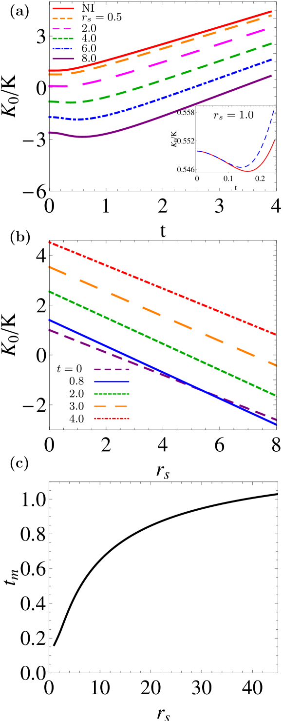
Figure 1: (color online) (a) Calculated $K_{0}/K$ in 2DEG as a function of rescaled temperature $t$ for different values of $r_{s}$. The inset presents $K_{0}/K$ in the low temperature regime. The dashed and solid lines are corresponding to the analytical results (given in Eq. 16) and the numerical results, respectively. (b) The inverse compressibility $K_{0}/K$ in 2DEG as a function of $r_{s}$ for different values of rescaled temperature $t$. (c) Calculated $t_{m}$, where the minimum of $K_{0}/K$ occurs, as a function of $r_{s}$.

In Fig. 1(a), we show the calculated inverse compressibility $K_{0}/K$ as a function of rescaled temperature $t$ for six different values of $r_{s}$. The red solid line corresponds to the non-interacting case ($K_{ni}$) without the exchange interaction. As shown in Sec. II.2 $K_{ni}^{-1}(T)\sim h(t)\sim t$ for $t\rightarrow\infty$ increases linearly in the high temperature classical limit. For finite $r_{s}$ the zero temperature inverse compressibility decreases with $r_{s}$ and eventually becomes negative (if $r_{s}>\pi/\sqrt{2}$) due to the exchange energy. As shown in Fig. 1(a) $K_{0}/K$ is not a monotonic function of rescaled temperature $t$. As $t$ increases from zero $K^{-1}(t)$ initially decreases since the kinetic energy term is exponentially suppressed due to the Fermi surface restriction, but the exchange term keeps decreasing as $t^{2}\ln t$. After reaching the minimum value at an $r_{s}$-dependent characteristic temperature $t_{m}$, $K^{-1}$ increases linearly at high temperatures. This non-monotonic behavior becomes stronger at higher $r_{s}$. More interestingly the negative value of $K^{-1}$ at low temperature and high $r_{s}$ reverses its sign as the temperature increases. At high enough temperatures, where the kinetic energy dominates over the interaction energy, the system always has a positive compressibility, but typically strongly suppressed in magnitude from $K_{ni}^{-1}$ except for $t\rightarrow\infty$. Thus, many-body effects manifest strongly in the compressibility even for $T>T_{F}$ in most situations.

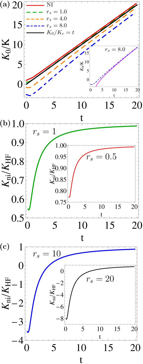
Figure 2: (color online) (a) Calculated $K_{0}/K$ as a function of $t$ for $r_{s}=1,4,8$ comparing the HF result with the non-interacting result $K_{0}/K_{ni}=h(t)$ as in Eq. 11 and the pure classical result $K_{0}/K_{c}=t$. Inset shows the HF result and the asymptotic form for the high temperature $K_{0}/K$ as in Eq. 18 with $r_{s}=8$. (b) and (c) show $K_{ni}/K_{HF}$ for $r_{s}=0.5$, $1.0$, $10$, $20$ for $t=0\sim 20$.

In Fig. 1(b), we show our numerically calculated inverse compressibility $K_{0}/K$ as a function of $r_{s}$ for different values of the rescaled temperature $t$. It is clear that the interacting $K_{0}/K$ manifests monotonically stronger many-body effects with increasing $r_{s}$. The curves for $t=0$ and $t=0.8$ cross each other at finite value of $r_{s}$, which corresponds to the non-monotonic temperature dependence of inverse compressibility $K_{0}/K$ in the low temperature regime. As an inset in Fig. 1(a) we explicitly show a quantitative comparison between our derived low-$T$ asymptotic formula (Eq. 16) and the exact numerical HFA results verifying the presence of the $t^{2}\ln t$ term, which leads to the low-$t$ minimum, in the HF $K_{0}/K$. In Fig. 1(c), we show as a function of $r_{s}$ our numerically calculated value of $t(\equiv T/T_{F})=t_{m}$ where the low-$t$ minimum of $K_{0}/K$ occurs. We note that although $t_{m}$ increases monotonically with increasing (decreasing) $r_{s}$ (density), this increase is sublinear implying that the actual temperature (in Kelvin) $T_{m}$, where the minimum occurs, decreases (increases) with decreasing (increasing) carrier density $n$ since $T_{F}\propto n$ and $r_{s}\propto n^{-1/2}$. This means that the experimental observation of this non-monotonicity of $K_{0}/K$ as a function of temperature may be extremely difficult, if not impossible, with the experimental $K_{0}/K$ manifesting only a monotonic increase with increasing temperature at all densities. The experimental observation is further hampered by two additional complications: (1) the actual decrease in the magnitude of $K_{0}/K$ associated with the shallow minimum is rather small ($<10\%$); (2) the low-density, large-$r_{s}$ regime of the 2D system often develops strong disorder-driven density inhomogeneity.

In Fig. 2 we compare our numerical results with our high-temperature analytic theory as given in Eq. 18. The purely classical compressibility $K_{c}(T)$ is given by $K_{0}/K_{c}=t$, which is the $t(=T/T_{F})\rightarrow\infty$ limit of $K_{0}/K_{ni}\equiv h(t)=(1-e^{-1/t})^{-1}$, as given in Eq. 11. We note that the exchange correction to the non-interacting result, as given in Eq. 18 falls off very slowly as $r_{s}t^{-1/2}\sim 1/\sqrt{T}$. In Fig. 2(a) we show calculated $K_{0}/K$ in the $t=0-20$ range for $r_{s}=1,4,8$ comparing the HF result with the non-interacting result $K_{0}/K_{ni}=h(t)$ as in Eq. 11, and the pure classical result $K_{0}/K_{c}=t$. For the sake of comparison, we also show (for $r_{s}=8$) the corresponding high-temperature HFA result as in Eq. 18. The interesting point to note here is that, as can be seen from Eq. 18, the quantum exchange correction is quantitatively substantial even at a temperature $T\gg T_{F}$ for large $r_{s}$ with the HFA results being quantitatively well below (by $\sim 20\%$) the classical result even for $T=20T_{F}$. Although this appears somewhat counter-intuitive, the importance of quantum interaction persisting to high temperatures ($T\gg T_{F}$) for large $r_{s}$ can be understood by considering the relative magnitudes of the three dimensionless energy parameters $r_{s}\equiv U/E_{F}$, $t\equiv T/T_{F}$, and $\Gamma\equiv U/k_{B}T$ that control the physics of an interacting quantum system – we note that $r_{s}$, $t$, $\Gamma$ are not independent parameters since $t\equiv r_{s}/\Gamma$. The classical noninteracting limit requires both $t$, $\Gamma^{-1}\gg 1$ which necessitates $t\gg r_{s}$ as well. Thus one condition for the classical limit is $t\gg r_{s}$ when $r_{s}>1$ (and $t\gg 1$ for $r_{s}<1$), which is much stronger than $t\gg 1$ when $r_{s}$ is large! In Fig. 2(b) and (c) we show $K_{ni}/K_{HF}$ for $r_{s}=0.5$, $1.0$, $10$, $20$ for $t=0\sim 20$ to emphasize that the exchange correction to the inverse compressibility is substantial in magnitude even for $T\gg T_{F}$.

II.4 Results for 2D GaAs systems

Since there has been considerable experimental activityEisenstein et al. (1992, 1994); Millard et al. (1997); Shapira et al. (1996) in measuring the 2D compressibility of both electronsEisenstein et al. (1992, 1994); Millard et al. (1997) and holesShapira et al. (1996) in GaAs-based two-dimensional semiconductor systems, we provide in this section a set of numerical results for the HF compressibility of 2D GaAs systems (electrons and holes) as a function of carrier density ($n$ in the unit of cm^-2) and temperature ($T$ in K). The parameters used in these numerical calculations are for electrons (holes): $m=0.07(0.4)m_{e}$; $g=2$ (i.e., $g_{s}=2$, $g_{v}=1$); $\kappa=13$, where $m_{e}$ is the free electron mass in vacuum and $\kappa$ is the background lattice dielectric constant of GaAs-AlGaAs heterostructure. There is no valley degeneracy ($g_{v}=1$) in GaAs, and we consider the spin-degenerate ($g_{s}=2$) zero-magnetic field situation.

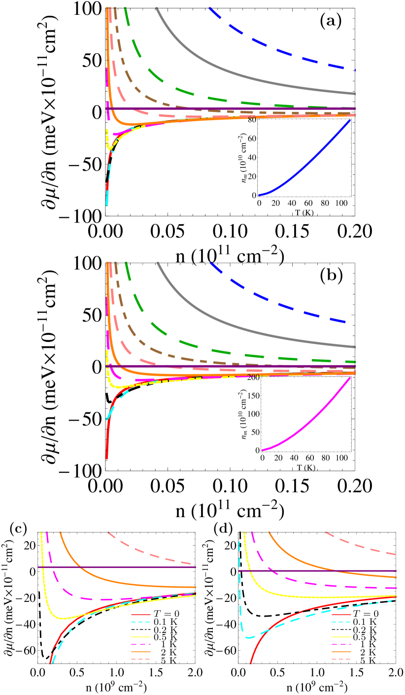
Figure 3: (color online) (a) and (b) Calculated $d\mu/dn\equiv(Kn^{2})^{-1}$ in the HFA for 2D GaAs electrons ($m=0.07m_{e}$) and holes ($m=0.4m_{e}$) respectively for $T=0,0.1,0.2,0.5,1,2,5,10,20,50,100$ K (from bottom to top). The solid horizontal line corresponds to the non-interacting $T=0$ result, $d\mu/dn\equiv[D_{0}(E_{F})]^{-1}$. Insets of (a) and (b): Calculated $n_{m}$, where the minimum of $d\mu/dn$ occurs, as a function of $T$ for electrons and holes respectively. (c) and (d) Zoom-in figures for the low-density parts of $d\mu/dn$ versus $n$ for 2D GaAs electrons and holes respectively.

In Fig. 3(a) and (b) we show our calculated $d\mu/dn\equiv(Kn^{2})^{-1}$ in the HFA for 2D GaAs electrons and holes respectively for $T=0,0.1,0.2,0.5,1,2,5,10,20,50,100$ K. The corresponding non-interacting $T=0$ result, $d\mu/dn\equiv[D_{0}(E_{F})]^{-1}=0.24(m_{e}/m)10^{-11}$ meVcm², is also shown as a constant horizontal line in each figure. The calculated temperature dependence is stronger for the holes than the electrons in Fig. 3 since the scale for the $T$-dependence, $T_{F}$, is much smaller (almost by a factor of six for the same density) for the holes compared with the electrons because of the large difference in the two effective masses ($0.07$ versus $0.4$). For $n=2\times 10^{10}$ cm^-2: $T^{e}_{F}=8.3$ K, $T^{h}_{F}=1.5$ K. Of course the qualitative behavior of $K(n,T)$ is the same for both electrons and holes, it is only that the temperature scale for the holes is lower.

The qualitative behavior of $d\mu/dn$ as a function density ($n$) and temperature ($T$) as shown in Fig. 3 is in very good agreement with experimental resultsShapira et al. (1996), showing that the temperature dependence of compressibility can indeed be very important in samples with low densities (and consequently with low $T_{F}$), particularly for holes because of their large effective mass. We note that $T_{F}=41.5$ K (electrons) and $7.3$ K (holes) for a density of $n=10^{11}$ cm^-2 (and $T_{F}\propto n$).

A particular qualitative feature of Fig. 3 deserves special attention: $d\mu/dn(\propto K^{-1})$ as a function of $n$ for a fixed temperature shows a very sharp upward turn with well-defined minimum at low densities, particularly for the low-$T$ results. This striking low-$n$ (and low-$T$) non-monotonicity arises from a quantum-classical crossover effect which turns on when $T_{F}(n)<T$ from being $T_{F}>T$ at some density and can therefore only be seen for low-$T$ and low-$n$ results. The minimum occurs at a density $n_{m}$ which we plot as a function of temperature $T$ in the inset showing that $n_{m}$ increases with increasing $T$. To further emphasize this interesting behavior, we show in Fig. 3(c) and (d), the low-density parts of $d\mu/dn$ versus $n$ for a few low $T$ values where the minimum is clearly visible. This sharp increase of $K^{-1}$ or $d\mu/dn$ for low density (and low temperature) has been experimentally observed in 2D GaAs systems, and has often been associated with the 2D metal-insulator-transition (MIT) driven by disorder. By contrast, our theory does not include disorder effects, we only include finite-temperature effects which are, of course, very strong at low densities where $T_{F}(n)<T$. The intuition based on the $T=0$ theory of compressibility clearly must fail at some low density (i.e., for $T_{F}(n)\lesssim T$) since the $T=0$ limit of $K^{-1}$ becomes large (in magnitude) and negative at very low $n$ whereas the finite-$T$ theory (for any finite $T$) predicts that at the lowest densities, where $T_{F}(n)<T$, $K^{-1}$ must become large and positive (i.e., the classical behavior for $T\gg T_{F}$), in fact eventually diverging as $T/T_{F}$ for $T\gg T_{F}$! We believe, based on the results presented in Fig. 3, that experimentalists should re-investigate the older data for $K^{-1}$ at low densities where finite temperature effects may be playing a significant role. There are some recent experimental results Ref.[Gao, ] supporting our finding, but more experimental data are necessary in the interacting low density and low temperature regime to settle this question definitively.

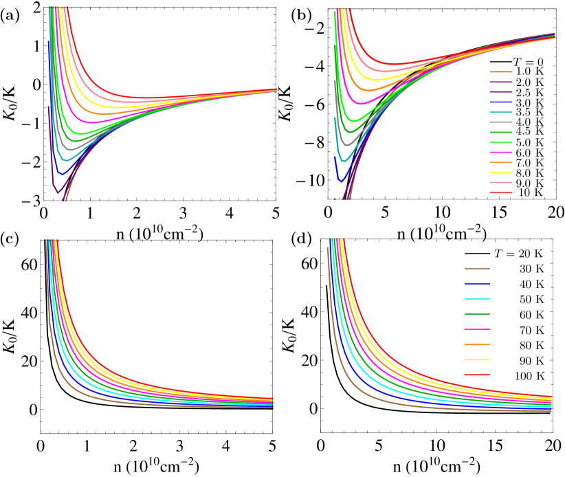
Figure 4: (color online) (a) and (b) Calculated $K_{0}/K$ as a function of carrier density in the HFA for electrons ($m=0.07m_{e}$) and holes ($m=0.4m_{e}$), respectively, over a wide range of temperature $T=0-10$ K. (c) and (d) show the high-$T$ behavior ($T=20-100$ K) of $K_{0}/K$ for electrons and holes respectively. The temperature increases from bottom to top in each figure.

Given the possible qualitative importance of finite temperature corrections to the 2D compressibility as discussed above (and shown in Fig. 3), we provide in Fig. 4 the calculated $K_{0}/K$ in the HFA for both electrons (Fig. 4(a)) and holes (Fig. 4(b)) over a wide range of density and temperature. The non-monotonicity apparent for higher-$T$ results in Figs. 4(a) and (b) particularly for the hole data, is actually present in all the curves except that the non-monotonicity manifests itself at much lower density than the range covered in Fig. 4 for the curves that simply look like that $K_{0}/K$ keeps on decreasing with density monotonically. In Figs. 4(c) and (d) we show the high-$T$ behavior ($T=20-100$ K) of $K_{0}/K$.

In Fig. 5, we show our calculated compressibility for 2D GaAs electrons and holes as a function of temperature for a few densities. Figs. 5(a) and (b) correspond to electrons showing $K_{0}/K$ as a function of temperature respectively over a wide $T=0-100$ K range [5(a)] and a narrow low temperature range $T=0-5$ K [5(b)] whereas Figs. 5(c) and (d) show the same for 2D holes in GaAs. In Figs. 5(b) and (d), we show a comparison between our low-$T$ analytical and numerical results also. The important point to note in Fig. 5 is that the low-temperature minimum should be observable in 2D semiconductor systems in careful measurements of $K_{0}/K$ as a function of temperature provided disorder effects are unimportant, i.e., highest-mobility samples are used for the study. Lower density samples would typically manifest deeper minima as can be seen in Fig. 5.

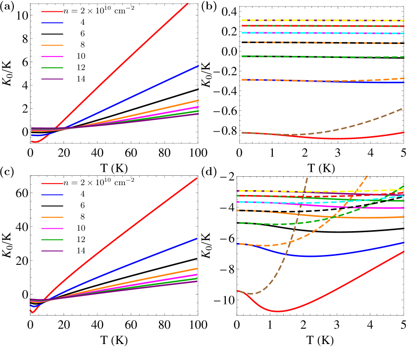
Figure 5: (color online) Calculated $K_{0}/K$ in the HFA as a function of temperature for various densities. Figs. (a) and (b) are for electrons($m=0.07m_{e}$), (c) and (d) are for holes($m=0.4m_{e}$). (a) and (c) show $K_{0}/K$ in the HFA for a wide range of temperature ($T=0-100$ K) for various densities $n=2,\ 4,\ 6,\ 8,\ 10,\ 12,\ 14\times 10^{10}$ cm^-2 (from top to bottom). (b) and (d) show $K_{0}/K$ at low temperatures ($T=0-5$ K) for various densities $n=2,\ 4,\ 6,\ 8,\ 10,\ 12,\ 14\times 10^{10}$ cm^-2 (from bottom to top) and compare the low-T analytical results (dashed lines) and numerical results (solid lines).

III Compressibility in graphene

In this section, we theoretically calculate the finite temperature compressibility of monolayer graphene including exchange interaction effects. It has been shown that the HFA is an excellent quantitative approximation due to the small contribution of the correlation energy in grapheneHwang et al. (2007). We focus on extrinsic graphene, i.e., gated or doped graphene with a tunable 2D free carrier density $n$ of electrons (holes) in the conduction (valence) band, i.e., the chemical potential $\mu$ being positive (negative). For undoped (intrinsic) graphene the chemical potential is zero even at finite temperatures, which gives rise to a logarithmically divergent compressibility if disorder effects are neglected Martin et al. (2008); Abergel et al. (2011). The basic feature of graphene compressibility and its functional dependence on density have been well studied in the literature at $T=0$Hwang et al. (2007); Abergel et al. (2011).

We use the same definition for the compressibility given in Sec. II. However, there are two main differences between the usual 2D semiconductor and graphene. The first one is the difference between their energy dispersion relation: 2D semiconductor has parabolic dispersion relation while graphene has linear dispersion. The kinetic energy in graphene is given by $\epsilon_{k,s}=sv_{F}|k|$, where $|k|$ is the wave vector with respect to the Dirac point, $v_{F}$ is the Fermi velocity with the value of $v_{F}\sim 10^{8}$ cm/s and $s=\pm 1$ for the conduction and valence band respectively. The second difference is that we need to consider the contribution from valence band electrons in graphene because graphene is a gapless semiconductor so that the valence band and the conduction band touch each other at the Dirac point. In graphene the total degeneracy $g=4$ (from spin degeneracy $g_{s}=2$ and valley degeneracy $g_{v}=2$).

Since the non-interacting chemical potential of graphene is $\mu_{0}=E_{F}=\hbar v_{F}k_{F}$ at zero temperature the corresponding non-interacting inverse compressibility is given by

$$K_{0}^{-1}=n^{2}\pi\hbar v_{F}/(2k_{F}),$$ (19)

where we use $g=4$ and the electron density is related to the Fermi wave vector as $k_{F}^{2}=\pi n$. Unlike the regular 2D systems, noninteracting $d\mu/dn$ in graphene is density dependent (i.e. $d\mu/dn\propto n^{-1/2}$) due to the linear energy dispersion of graphene.

The chemical potential within HFA is the sum of the non-interacting kinetic energy part and the exchange self-energy part. The exchange self-energy for graphene is given asHwang et al. (2007):

$$\Sigma_{x,s}(k)=-\sum_{s^{\prime}}\int\frac{d^{2}k^{\prime}}{(2\pi)^{2}}V\left(\left|k-k^{\prime}\right|\right)n_{F}\left(\xi_{\bm{k}^{\prime},s^{\prime}}\right)F_{s,s^{\prime}}\left(\bm{k},\bm{k}^{\prime}\right)$$ (20)

where $s,s^{\prime}=\pm 1$ indicates the band indices, $V\left(q\right)=2\pi e^{2}/(\kappa q)$ is the bare Coulomb interaction ($\kappa$ is the background dielectric constant), and $F_{ss^{\prime}}(\bm{k},\bm{k}^{\prime})=(1+ss^{\prime}\cos\theta_{\bm{k}\bm{k}^{\prime}})/2$ arises from the wavefunction overlap factor where $\theta_{\bm{k}\bm{k}^{\prime}}$ is the angle between $\bm{k}$ and $\bm{k}^{\prime}$. In regular (i.e., non-chiral) 2D systems, $F\equiv 1$, but in graphene, which is a chiral material, the chiral factor $F$ is important due to the underlying pseudospin dynamics. With Eq. (20) we calculate the interacting compressibility of graphene at finite temperatures. Since the zero temperature exchange self energy can be calculated analyticallyHwang et al. (2007) we first consider the zero temperature compressibility as the starting point of our discussion.

III.1 Zero temperature compressibility

At $T=0$, the Fermi distribution function in Eq. 20 becomes $n_{F}(\xi)=\theta(E_{F}-\xi)$. We divide the exchange self-energy into two partsHwang et al. (2007): one from the intraband transition $\Sigma^{\rm int}_{x}$, and the other from the interband transition $\Sigma^{\rm ext}_{x}$. That is, $\Sigma_{{\rm x},s}(k)=\Sigma_{{\rm x},s}^{\rm int}(k)+\Sigma_{{\rm x},s}^{\rm ext}(k)$, where

$$\begin{array}[]{l l l }\Sigma_{{\rm x},s}^{\rm int}(k)=-\int\dfrac{d\bm{q}}{(2\pi)^{2}}V_{c}(\bm{q})\,F_{s,-}(\bm{k},\bm{k}-\bm{q});\\ \\ \Sigma_{{\rm x},s}^{\rm ext}(k)=-\sum_{s^{\prime}}\int\dfrac{d\bm{q}}{(2\pi)^{2}}\delta n_{F}(\xi_{\bm{k}-\bm{q},s^{\prime}})V_{c}(\bm{q})\,F_{ss^{\prime}}(\bm{k},\bm{k}-\bm{q})\end{array}$$ (21)

where $\delta n_{F}(\xi_{\bm{k}-\bm{q},s^{\prime}})=n_{F}(\xi_{\bm{k}-\bm{q},s^{\prime}})-\frac{1}{2}(1-s^{\prime})$ is the difference in the electron occupation from the intrinsic $T=0$ case.

After some algebra (the detail of the derivation is given in Ref. [Hwang et al., 2007]), we find the density dependent exchange contribution to the inverse compressibility $K_{0}/K$ at zero temperature

$$\frac{K_{0}}{K}=1+r_{s}\Big{[}\dfrac{1}{4}\ln\Big{(}\dfrac{4}{y}\Big{)}-\dfrac{3}{8}-\frac{1}{2\pi}-\frac{C}{\pi}\Big{]}$$ (22)

where $y=k_{F}/k_{c}$ with a momentum cut-off $k_{c}\sim a^{-1}$ where $a$ is a lattice constant of graphene, $C\approx 0.916$ is Catalan’s constant, and $r_{s}=\dfrac{e^{2}}{\hbar v_{F}\kappa}$ is the graphene coupling constant (or fine structure constant). We note that the $\ln y\equiv\ln(k_{F}/k_{c})$ term takes care of the divergent compressibility of intrinsic graphene which does not enter our discussion in any significant manner. Unlike in 2D systems, where the interaction parameter $r_{s}\sim n^{-1/2}$, for graphene $r_{s}$ is a constant in density due to its linear energy dispersion. However, by adjusting the background dielectric constant ($\kappa$) we can vary the $r_{s}$ value, from $r_{s}=2.2$ (for $\kappa=1$, graphene suspended in vacuum) to very small $r_{s}$ by making $\kappa$ very large. For graphene on SiO₂, $r_{s}=0.8$. Note that unlike ordinary 2D systems the calculated graphene compressibility with the exchange correction is always positive, which has recently been measured by several different techniques recently Eisenstein et al. (1992, 1994).

III.2 Finite temperature compressibility

In this subsection, we present the theoretical formalism of the finite temperature $K_{0}/K$ and its asymptotic analytical formula at low temperatures ($t\ll 1$). We consider extrinsic graphene with $E_{F}>0$ and concentrate on the situation with the chemical potential lying in the conduction band with no loss of generality.

The finite temperature chemical potential (without exchange energy) $\mu_{0}$ must be calculated by the conservation of the total electron density, i.e. $n(T)=n(T=0)+p(T)$, where $n(T)$ and $p(T)$ are the electron and hole density at $T$, respectively. They are given by

$$n(T)=g\int\frac{d^{2}p}{(2\pi)^{2}}\frac{1}{\exp[\beta(\varepsilon_{p}-\mu)]+1}$$ (23)

and

$$p(T)=g\int\frac{d^{2}p}{(2\pi)^{2}}\frac{1}{\exp[-\beta(\varepsilon_{p}-\mu)]+1},$$ (24)

where $g$ is the total degeneracy and $\beta=1/k_{B}T$. Thus, we have the self consistent equation for $\mu$ as

$$\frac{1}{2}\left(\frac{T_{F}}{T}\right)^{2}=F_{1}\left(\beta{\mu}\right)-F_{1}\left(-\beta{\mu}\right),$$ (25)

where $F_{n}(x)$ is given by

$$F_{n}(x)=\int_{0}^{\infty}\frac{t^{n}dt}{1+\exp(t-x)}.$$ (26)

Then we obtain the non-interacting chemical potential for both low and high temperature limits for graphene as

$$\mu_{0}(T) \approx E_{F}\left[1-\frac{\pi^{2}}{6}\left(\frac{T}{T_{F}}\right)^{2}\right]\;\;{\rm for}\;T/T_{F}\ll 1$$ (27)

$$\mu_{0}(T) \approx \frac{E_{F}}{4\ln 2}\frac{T_{F}}{T}\hskip 62.59596pt{\rm for}\;T/T_{F}\gg 1.$$ (28)

With Eqs. (27) and (28) we can find the noninteracting graphene compressibility at low temperatures and at high temperatures, respectively. Let $\mu_{0}/E_{F}\equiv\tilde{\mu_{0}}$ and $t=T/T_{F}$, then the non-interacting part of the inverse compressibility can be written as

$$\frac{K_{0}}{K_{ni}(T)} = 1+\frac{\pi^{2}t^{2}}{6}\hskip 28.45274pt{\rm for}\;t\ll 1,$$ (29)

$$\frac{K_{0}}{K_{ni}(T)} = \frac{1}{2\ln 2}\frac{1}{t}\;\hskip 28.45274pt{\rm for}\;t\gg 1.$$ (30)

Thus the leading order correction to the inverse compressibility $K_{ni}(T)^{-1}$ increases quadratically at low temperatures and then it decreases inverse linearly at high temperatures. This fact indicates that the graphene compressibility shows the opposite behavior to the ordinary 2D systems as shown in Sec. II, where the inverse compressibility of 2D systems decreases first and then increases as the temperature increases. We emphasize that this qualitative difference in the noninteracting finite-$T$ compressibility between 2D systems and monolayer graphene arises both from the linear, chiral energy dispersion of graphene and from its gaplessness allowing for thermal excitations of conduction valence band electron-hole pairs at finite $T$.

Now we calculate the full compressibility at low temperatures, including the exchange energy. As done for the zero temperature case, the exchange self energy of graphene can be separated into contributions from the intrinsic part $\Sigma^{\rm int}_{x}$ and the extrinsic part $\Sigma^{\rm ext}_{x}$Hwang and Das Sarma (2009). We can see that the first term in Eq. (34) is $\Sigma^{\rm int}_{x}$ while the second term is $\Sigma^{\rm ext}_{x}$. For $\mu>0$ the Hartree-Fock self energy in graphene at finite temperature becomes

$$\begin{array}[]{l c c c c c c}\Sigma^{\rm int}_{x}(k,T)=-\dfrac{e^{2}}{2\pi\kappa}\int\int\frac{qdqd\theta}{|k-q|}\frac{1}{\exp\left(\beta\left(-\hbar v_{F}q-\mu\right)\right)+1}\frac{1-\text{cos$\theta$}}{2}\\ \\ \Sigma^{\rm ext}_{x}(k,T)=-\dfrac{e^{2}}{2\pi\kappa}\int\int\frac{qdqd\theta}{|k-q|}\frac{1}{\exp\left(\beta\left(\hbar v_{F}q-\mu_{0}\right)\right)+1}\frac{1+\text{cos$\theta$}}{2}\end{array}$$ (34)

The intrinsic exchange self-energy $\Sigma^{\rm int}_{x}$ in Eq. (34) can be derived by using the fact that the exponential term in $\Sigma^{\rm int}_{x}$ is exponentially suppressed and almost equal to $1$ in the low temperature limit. Then, we have Hwang et al. (2007)

$$\begin{array}[]{l l l }\Sigma^{\rm int}_{x}(T)=\dfrac{e^{2}k_{F}}{\pi\kappa}\left[-\dfrac{E(y)}{y}+\dfrac{\pi}{4}\ln(\dfrac{4}{y})-\dfrac{\pi}{8}\right.\\ \ \ \ \ \ \ \ \ \ \ \ -\left.\int_{0}^{y}\dfrac{dx}{x^{3}}(K_{1}(x)-E(x)-\dfrac{\pi}{4}x^{2})\right]+O(e^{-\beta}),\end{array}$$ (35)

where $y=k_{F}/k_{c}\ll 1$, $K_{1}(x)$ and $E(x)$ are the complete elliptic integral of the first and second kinds, respectively. Note that the leading order temperature correction of the intrinsic exchange self-energy at low temperatures is exponentially suppressed. On the other hand, the extrinsic part of the exchange self-energy becomes

$$\Sigma^{\rm ext}_{x}(T)=-\dfrac{e^{2}k_{F}}{\pi\kappa}\left[C+\dfrac{1}{2}-\dfrac{B_{g}}{12}\pi^{2}t^{2}+\dfrac{1}{12}\pi^{2}t^{2}\ln t\right]$$ (36)

where $C\approx 0.916$ is Catalan’s constant, $B_{g}=-1+2\gamma-12\ln(G)+\ln\left(\frac{128}{\pi}\right)\approx 0.877$ where $G\simeq 1.282$ is Glaisher’s constant and $\gamma\simeq 0.577$ is Euler’s constant. Differentiating the total chemical potential with respect to the density, we have the asymptotic form of inverse compressibility in the low temperature limit

$$\dfrac{K_{0}}{K(T)}=f(t) + r_{s}\Big{[}\dfrac{1}{4}\ln\Big{(}\dfrac{4}{y}\Big{)}-\dfrac{3}{8}-\dfrac{C}{\pi}-\dfrac{1}{2\pi}$$ (37)

$$- \dfrac{\pi t^{2}}{12}(B_{g}-1)+\frac{\pi}{12}t^{2}\ln t\Big{]},$$

where $f(t)\equiv 1+\frac{\pi^{2}t^{2}}{6}$ is the non-interacting part of the inverse compressibility given in Eq. (29). In the low temperature limit the leading order temperature correction to the total inverse compressibility is the same as that in the 2D semiconductor system due to the exchange energy, i.e., $t^{2}\ln t$. However, the logarithmic correction can be detected only at very low temperatures ($t<0.01$). In general, the $t^{2}$ correction from the non-interacting part dominates at low temperatures ($t>0.01$) and the positive coefficient of $t^{2}$ term gives rise to increasing behavior of $K^{-1}$ with temperature. Our asymptotic results at low temperatures agree very well with the full numerical results shown in Fig. 6(a). The results provided in this section generalize the existing graphene literature on compressibilityHwang et al. (2007) to finite temperatures.

III.3 Numerical results of graphene compressibility

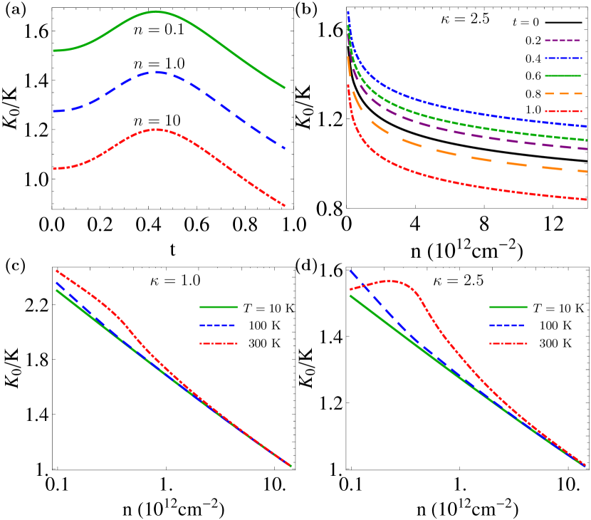
Figure 6: (color online). (a) Calculated $K_{0}/K$ in graphene as a function of temperature $t$ for three different values of density in the units of $10^{12}$cm^-2. (b) Calculated $K_{0}/K$ in graphene as a function of carrier density $n$ for six different values of rescaled temperature $t$. In this calculation the momentum cut-off $k_{c}=1/a$ ($a=2.46$ Å) and $\kappa=2.5$ are used. (c) The semi-log plot of $K_{0}/K$ versus carrier density with different temperatures $T$ for $\kappa=1$ and (d) for $\kappa=2.5$.

In this subsection, we present our numerical results of finite temperature compressibility in graphene. Throughout this section, we use $v_{F}=10^{8}$ cm/s and the wave vector cut-off $k_{c}=1/a$ ($a=2.46$ Å). We show results for suspended graphene ($\kappa\sim 1.0$) and for graphene on SiO₂ ($\kappa\sim 2.5$). In Fig. 6(a) we show the temperature dependence of the total inverse compressibility $K_{0}/K$ for three different values of carrier density $n=0.1\times 10^{12}cm^{-2}$, $n=1\times 10^{12}$ cm^-2, $n=10.0\times 10^{12}$ cm^-2 with dielectric constant $\kappa=2.5$ (corresponding to graphene on the Si/SiO₂ substrate). We can clearly see that the temperature dependence is non-monotonic and this non-monotonic behavior mostly comes from the non-interacting compressibility, which is different from the 2D semiconductor case. Unlike the 2D parabolic-band case, the compressibility in graphene does not change sign in the range of experimentally relevant parameters and typically exchange corrections are always quantitatively small ($\lesssim 20\%$). We show the carrier density dependence of $K_{0}/K$ in Fig. 6(b), where the $K_{0}/K$ is a monotonically decreasing function of carrier density for small values of $t$ ($T\simeq 400K$ for $t=1$ and $n=0.1\times 10^{12}cm^{-2}$). In Fig. 6(c) and (d), we present the calculated $K_{0}/K$ as a function of carrier density for different temperatures. For fixed temperatures, $K_{0}/K$ is a decreasing function of $n$ at higher carrier density, which corresponds to the low temperature limit manifesting $n^{-1}$ density dependence. On the other hand, at lower carrier density, $K_{0}/K$ has $n^{1/2}$ density dependence, which corresponds to the high temperature limit and the main contribution to $K_{0}/K$ comes from the non-interacting part (see Eq. 30).

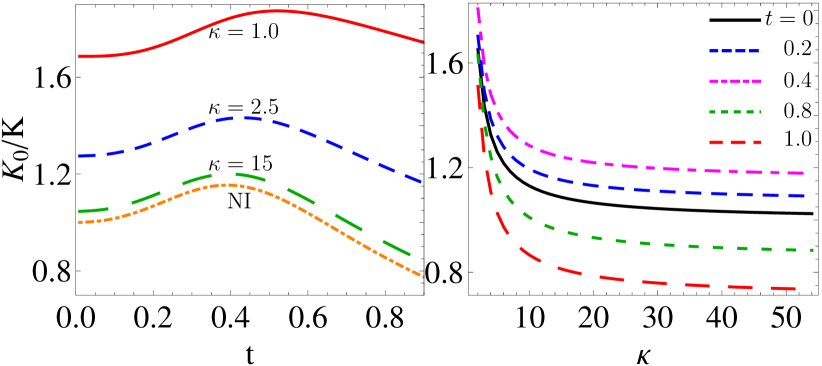
Figure 7: (color online). (a) Calculated $K_{0}/K$ in monolayer graphene as a function of temperature $t$ for three different values of background dielectric constant within HFA for carrier density $n=10^{12}$cm^-2. The dot-dashed (orange) line presents the temperature dependence of the non-interacting $K_{0}/K$. (b) Calculated $K_{0}/K$ in monolayer graphene as a function of the background dielectric constant $\kappa$ for a few fixed values of $t$. $k_{c}=1/a$ ($a=2.46$Å).

In Fig. 7, we compare the temperature dependence for different values of background dielectric constant $\kappa=1$ (i.e. graphene in vacuum), $\kappa=2.5$ (graphene on Si/SiO₂) and $\kappa=15$ (graphene on hafnium oxide HfO₂), respectively. The value of $r_{s}$ represents the fine structure constant of graphene which depends only on $\kappa$ and does not depend on the carrier density because of the linear energy dispersion. Larger dielectric constant corresponds to smaller values of $r_{s}$, which indicates a weak-coupling system in terms of electron-electron interactionHwang and Das Sarma (2009). Note that the trends of $K_{0}/K$ among different values of dielectric constant are similar. The larger the value of dielectric constant (the smaller the value of $r_{s}$), the less strong is the density dependence of $K_{0}/K$. We also show in this figure our calculated $K_{0}/K$ in HFA compared with the noninteracting $K_{0}/K$ as a function of the background dielectric constant $\kappa$ for a few fixed values of $t$. We could see that the inverse compressibility $K_{0}/K$ first increases as the temperature $t$ increases, reaches a maximum, and then decreases as the temperature $t$ further goes up. This non-monotonic behavior of $K_{0}/K$ dependence on the temperature is mainly due to the non-interacting part of the chemical potential, which is consistent with the calculation of the non-interacting part of the chemical potential (Eq.28). From Eq (28) we know that the temperature dependence of the chemical potential is $t^{2}$ (with a positive slope) at low temperatures while the temperature dependence of the chemical potential approximates as $1/t$ (with a negative slope) at higher temperatures. There must be an intermediate point at which the chemical potential changes its sign of slope and so does the compressibility $K$. Since $K^{-1}$ is the derivative of chemical potential with respect to $n$, it has similar temperature dependence as the chemical potential. Therefore, the non-interacting part of $K_{0}/K$ behaves as $t^{2}$ at low temperatures and then changes to $1/t$ behavior. The domination of graphene compressibility by noninteracting effects is just a direct manifestation of the weakness of electron-electron interaction in graphene compared with the 2D semiconductor case.

IV compressibility of BLG

In this section, we calculate the BLG compressibility within the HF approximation. There is some related theoretical work in the literature dealing with the problem of compressibility in BLG, Kusminskiy et al. (2008); Borghi et al. (2010); Abergel et al. (2011, ) but the specific and detailed temperature dependent compressibility presented in the current work is not available in the literature. To calculate BLG compressibility at finite temperatures we use the two-band approximation, which is valid for the low density limit. At high density, BLG dispersion approaches the linear energy dispersion of monolayer graphene as the Fermi energy becomes largeDas Sarma et al. (2011), and therefore the high-density BLG compressibility behaves similar to the MLG compressibility studied in the last section. It has been shown that the two band model presents the most important qualitative signatures of the BLG compressibility. Kusminskiy et al. (2008); Borghi et al. (2010); Sensarma et al. (2011); Abergel et al. (2011) For low density bilayer graphene within two-band model, the quadratic approximation is commonly used, i.e., $\xi_{k}=\hbar^{2}v_{F}^{2}k^{2}/\gamma_{1}=\hbar^{2}k^{2}/(2m)$, where $\gamma_{1}$ is the interlayer hopping parameter from the tight-binding approximation and $m=\gamma_{1}/(2v_{F}^{2})$ is the effective mass of the electrons. This dispersion comes from a low-energy effective theory of bilayer grapheneDas Sarma et al. (2011), which essentially discards the two split bands and confines electrons to those lattice sites not involved in the interlayer coupling. While the quadratic dispersion is relevant at low energies, the actual dispersion of the bands is hyperbolic. At large wave vectors, relevant at large densities, the dispersion is effectively linear and the system should behave like single layer graphene. Thus our results obtained in the previous section should be applicable to the high density BLG.

The exchange self energy of BLG is given by

$$\Sigma_{x,s}(k)=-\sum_{s^{\prime}}\sum_{{\bf k}^{\prime}}V_{{\bf k-k}^{\prime}}n_{F}(\xi_{{\bf k}^{\prime},s^{\prime}})F_{s,s^{\prime}}({\bf k},{\bf k}^{\prime}),$$ (38)

where $V_{\bf k-\bf k^{\prime}}=2\pi e^{2}/\kappa|\bf k-\bf k^{\prime}|$ is the Coulomb potential, $\xi_{\bf k}=k^{2}/2m$, $n_{F}(x)$ is the Fermi distribution function, and $F_{s,s^{\prime}}({\bf k},{\bf k^{\prime}})=(1+ss^{\prime}\cos(2\theta_{\bf k\bf k^{\prime}}))/2$ is the wave function overlap factor and $\theta_{kk^{\prime}}$ is the angle between $\bf k$ and $\bf k^{\prime}$. To get the explicit temperature dependence we rewrite Eq. (38) as

$$\Sigma_{x}(k) = \Sigma_{2D}(k)+\Sigma_{x}^{int}(k)$$ (39)

$$+ \frac{1}{2}\sum_{\bf k^{\prime}}V_{\bf k-\bf k^{\prime}}[f(\xi_{\bf k^{\prime}})+g(\xi_{\bf k^{\prime}})][1-\cos(2\theta)],$$

where $f(x)=1/(e^{\beta(x-\mu)}+1)$ and $g(x)=1/(e^{\beta(x+\mu)}+1)$, $\Sigma_{2D}(k)$ is the ordinary 2D self energy given in Eq. (5), and $\Sigma_{x}^{int}$ is given by

$$\Sigma_{x}^{int}(k) = -\int\frac{d^{2}k^{\prime}}{(2\pi)^{2}}V_{k-k^{\prime}}\frac{1-\cos(2\theta)}{2}$$

$$= \frac{2e^{2}k}{3\pi\kappa}\Big{[}\frac{\pi}{2}-p(z)+q(z)\Big{]}$$

where

$$p(z)=\begin{cases}\dfrac{(1+7z^{2})E(z)}{3z^{3}}&z\leq 1\\ \\ \dfrac{(1+7z^{2})E(1/z)}{3z^{2}}&z>1\end{cases}$$ (41)

and

$$q(z)=\begin{cases}\dfrac{(1+2z^{2}-3z^{4})K_{1}(z)}{3z^{3}}&z\leq 1\\ \\ \dfrac{4(z^{2}-1)K_{1}(1/z)}{3z^{2}}&z>1\end{cases}$$ (42)

Here $z=k/k_{c}$, $k_{c}\sim 1/a$ is the momentum cut-off (similar to the MLG situation) with a lattice constant $a$. $K_{1}(x)$ and $E(x)$ are the complete elliptic integral of the first and the second kind, respectively. Since we have studied $\Sigma_{2D}$ in Sec. II and $\Sigma_{x}^{int}$ is independent of temperature, the new feature of temperature dependent compressibility of BLG arises from the third term in Eq. (39), i.e.,

$$\Sigma_{x}^{(3)}(k)=\frac{1}{2}\sum_{k^{\prime}}V_{k-k^{\prime}}[f(\xi_{k^{\prime}})+g(\xi_{k^{\prime}})][1-\cos(2\theta)].$$ (43)

Then the total temperature dependent HFA chemical potential of BLG can be calculated to be

$$\mu(T)=E_{F}+\Sigma(k_{F},T).$$ (44)

IV.1 Zero temperature BLG compressibility

At $T=0$, using $f(x)=\theta(1-x)$ and $g(x)=0$ in Eq. (43), the exchange self-energy can be calculated as:

$$\Sigma_{x}(k) = -\frac{2e^{2}k_{F}}{\pi\kappa}E\left(\frac{k}{k_{F}}\right)+\frac{2e^{2}k}{3\pi\kappa}\Big{[}p\left(\frac{k}{k_{F}}\right)-q\left(\frac{k}{k_{F}}\right)$$ (45)

$$- p\left(\frac{k}{k_{c}}\right)+q\left(\frac{k}{k_{c}}\right)\Big{]}.$$

Then, the exchange self-energy at $k=k_{F}$ is given by

$$\Sigma_{x}(k_{F})=-\frac{2e^{2}k_{F}}{\pi\kappa}+\frac{2e^{2}k_{F}}{3\pi\kappa}\Big{[}\frac{8}{3}-p(y)+q(y)\Big{]}.$$ (46)

where $y=k_{F}/k_{c}$. The total chemical potential for BLG within HFA is then written as

$$\mu=E_{F}\left[1-\frac{r_{s}}{\pi}\left(\frac{2}{9}+\frac{2}{3}[p(y)-q(y)]\right)\right]$$ (47)

where $r_{s}=2e^{2}m/(\kappa k_{F})$ is the dimensionless BLG coupling. In the following numerical calculation, we use the the value of dielectric constant $\kappa=2.5$ and effective mass $m=0.03m_{e}$Das Sarma et al. (2011). Differentiating Eq. 47 with respect to $n$ and making use of the relation $k_{F}^{2}=\pi n$, we get the zero temperature BLG inverse compressibility within HFA

$$\frac{K_{0}}{K}=1-\frac{r_{s}}{\pi}\left(\frac{1}{9}+\frac{1}{3}[p(y)-q(y)]\right)+\frac{r_{s}}{\pi}w(y)$$ (48)

where $K_{0}$ is the non-interacting compressibility of BLG, given by

$$\frac{1}{K_{0}}=\frac{\pi n^{2}}{2m}.$$ (49)

and

$$w(y)=\begin{cases}\dfrac{1+y^{2}}{3y^{3}}E(y)+\dfrac{y^{2}-1}{3y^{3}}K_{1}(y)&y\leq 1\\ \\ \dfrac{1+y^{2}}{3y^{2}}E(1/y)+\dfrac{1-y^{2}}{3y^{2}}K_{1}(1/y)&y>1\end{cases}.$$ (50)

At low enough densities the zero temperature compressibility within HF approximation becomes negative similar to the corresponding 2D semiconductor system. The corresponding density is $n_{c}\sim 10^{10}$ $cm^{-2}$ or $r_{s}\sim 27$, for which the negative compressibility manifests itself. This is a very small (large) value of density ($r_{s}$) compared with the ordinary 2D case where the negative compressibility shows up for $r_{s}>2.2$. However the negative compressibility obtained in HFA has not been experimentally observed in bilayer graphene systemsHenriksen and Eisenstein (2010); Young et al. ; Martin et al. (2010). The non-negative compressibility may be attributed to correlation effects. It is shown that the contributions from exchange and correlation almost cancel each other out in BLG at low density, leaving a small positive compressibility at all densities in contrast to the corresponding 2DEG systems Eisenstein et al. (1992, 1994); Dultz and Jiang (2000); Ilani et al. (2000); Dultz et al. where the electronic compressibility can become negative at low densities. Borghi et al. (2010); Sensarma et al. (2011) The non-quadratic band structure also gives rise to significant affects on the compressibility as has recently been discussed in the literature. Abergel et al. (2011)

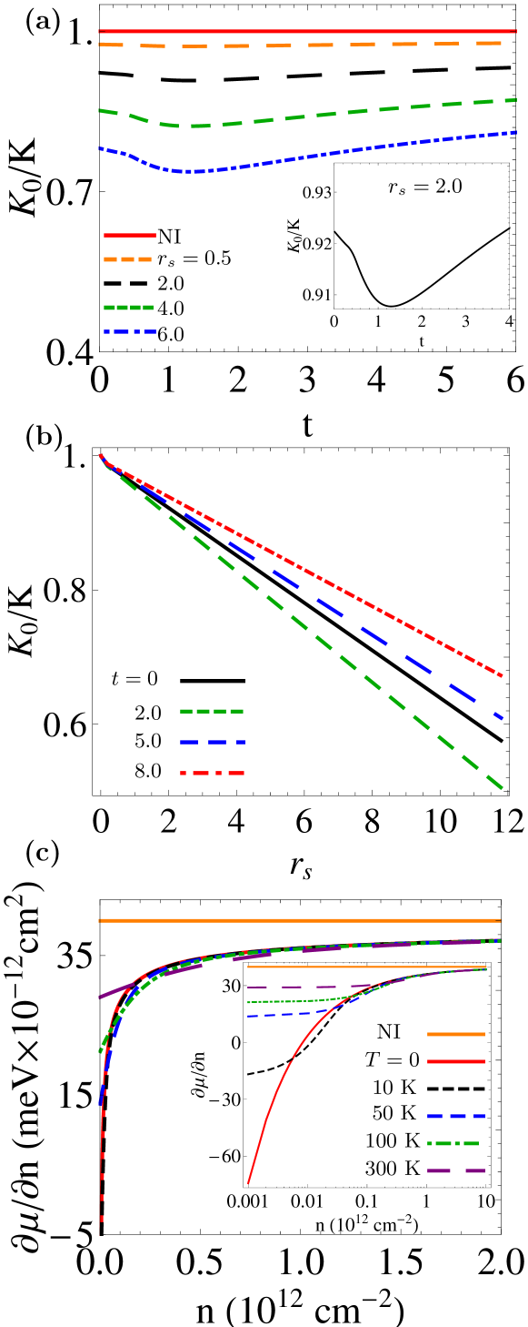
Figure 8: (color online) (a) Calculated $K_{0}/K$ in BLG as a function of temperature $t=T/T_{F}$ for different values of $r_{s}$. The inset presents $K_{0}/K$ for $r_{s}=2.0$ showing the non-monotonic behavior. $k_{c}=1/a$ ($a=2.46$ Å) and $\kappa=2.5$ are used. (b) The inverse compressibility $K_{0}/K$ in BLG as a function of $r_{s}$ for different values of temperature $t$. (c) $\partial\mu/\partial n$ in BLG versus carrier density $n$ for various temperatures. Inset shows the details in the low density limit in the semi-log scale.

IV.2 Finite temperature BLG compressibility

At finite temperatures the non-interacting chemical potential is temperature independent in BLG, i.e.,

$$\mu_{0}(T)=E_{F}.$$ (51)

Then the non-interacting compressibility of BLG is also temperature independent and is the same as the zero temperature compressibility given in Eq. (49)

$${K_{ni}(T)}=K_{0}.$$ (52)

At finite temperatures, the temperature dependence of BLG compressibility comes from the exchange contribution. This is very intriguing because the non-interacting kinetic energy dominates exchange self energy at high temperatures for both ordinary 2D systems and MLG. But in BLG the entire temperature dependence arises from the exchange energy! Thus, any experimentally observed temperature dependence in the BLG compressibility must entirely be a many-body effect, at least within the 2-band approximation (i.e., at not-too-high carrier densities).

Let us consider the exchange self energy, Eq. (39), at finite temperatures. The first term in Eq. (39) has been calculated in Sec. II [see Eq. (14)] and the second term is temperature independent. The third term [Eq. (43)] becomes in the low temperature limit $t=T/T_{F}\ll 1$:

$$\Sigma_{x}^{(3)}(k_{F})\simeq\frac{2e^{2}k_{F}}{3\pi\kappa}(\frac{8}{3}-\frac{\pi}{2}-\frac{\pi^{2}}{24}t^{2})+O(t^{4}).$$ (53)

Thus, we have the total HFA chemical potential in the low temperature limit

$$\mu(T) = E_{F}\left[1-\frac{r_{s}}{\pi}\left(\frac{2}{9}+\frac{2}{3}[p(y)-q(y)]\right)\right]$$ (54)

$$- E_{F}\frac{r_{s}}{\pi}\left[\frac{Bt^{2}}{4}+\frac{5\pi^{2}t^{2}}{72}-\frac{1}{48}\pi^{2}t^{2}\text{ln}\frac{16}{t}\right].$$

where $B=\frac{\pi^{2}}{12}[\ln(4\pi)+12\zeta^{\prime}(-1)]\approx 0.449$ and $\zeta^{\prime}(-1)$ is the derivative of the zeta function. Differentiating the asymptotic formula of chemical potential with respect to the density, we have the BLG $K_{0}/K$ for $t\ll 1$

$$\begin{array}[]{l l l}\dfrac{K_{0}}{K(T)}\simeq\dfrac{K_{0}}{K(T=0)}+\dfrac{r_{s}}{\pi}\Big{[}0.55t^{2}+\dfrac{\pi^{2}}{32}t^{2}\text{ln}t\Big{]}.\end{array}$$ (56)

where $K_{0}/K(T=0)$ has been derived in Eq. 48. We have the same leading order term $t^{2}\ln t$ arising from the exchange self-energy as the ordinary 2D system. Thus, at low temperatures the calculated inverse compressibility decreases as the temperature increases.

In the high temperature limit $T\gg T_{F}$, the chemical potential can be calculated to be:

$$\mu(T)=E_{F}\left[1-\frac{r_{s}}{\pi}\left(\frac{B_{1}}{\sqrt{t}}+\frac{2}{3}[p(y)-q(y)]\right)\right]$$ (57)

where $B_{1}=[-3\sqrt{2}\pi^{2}+8\left(-1+2\sqrt{2}\right)\sqrt{\pi}\zeta(\frac{3}{2})]/64\approx 0.4$ and $\zeta(x)$ is the zeta function. Then the inverse compressibility is given by

$$\frac{K_{0}}{K(T)}=1-\frac{r_{s}}{\pi}\left(\frac{B_{1}}{\sqrt{t}}+\frac{p(y)-q(y)}{3}-w(y)\right).$$ (58)

In the high temperature limit ($t\gg 1$) the inverse compressibility of the ordinary 2D systems increases linearly with temperature and approaches the non-interacting value. However, since the non-interacting compressibility of BLG is temperature independent and the most dominant exchange term decreases as $t^{-1/2}$, the high temperature inverse compressibility of BLG approaches the following high-temperature limit:

$$\frac{K_{0}}{K(T)}\Big{|}_{T\rightarrow\infty}=1-\frac{1}{8}\frac{a}{a_{B}},$$ (59)

where $a_{B}=\hbar^{2}\kappa/(me^{2})$ is the BLG effective Bohr radius. Since $a/a_{B}<1$ the negative inverse compressibility reverses its sign to the positive values at high temperatures and asymptotically approaches a smaller value than the zero temperature inverse compressibility. This intriguing result is purely a high-temperature manifestation of exchange effect within the 2-band BLG approximation.

In Fig. 8, we present our numerical results of temperature dependent inverse compressibility in BLG systems. In the calculation we use $k_{c}=1/a$ ($a=2.46$Å) and $\kappa=2.5$. As shown in Fig. 8 the calculated BLG inverse compressibility shows very weak temperature dependence. The weak non-monotonic behavior of temperature-dependent inverse compressibility is shown in the inset of Fig. 8(a). In Fig. 8(b), we present the inverse compressibility versus $r_{s}$. $K^{-1}$ decreases monotonically with $r_{s}$ and becomes negative at $r_{s}\sim 27$. In Fig. 8(c)) we show $\partial\mu/\partial n$ as a function of density and the inset shows the same figure in the semi-logarithm scale to show clearly the behavior at low densities. At densities $n\lesssim 10^{10}cm^{-2}$ the zero temperature $\partial\mu/\partial n$ is negative, but as temperature increases it reverses its sign at $t\approx[0.4/(\pi/r_{s}-a/8a_{B})]^{2}$. As temperature increases further it approaches $(\hbar^{2}\pi/2m)(1-a/8a_{B})$ regardless of density.

In Fig. 9, we show, for the purpose of comparison, the calculated $K_{0}/K$ for the 2D, MLG, and BLG systems as functions of $r_{s}$ and $t$ in order to demonstrate the qualitative difference between the results.

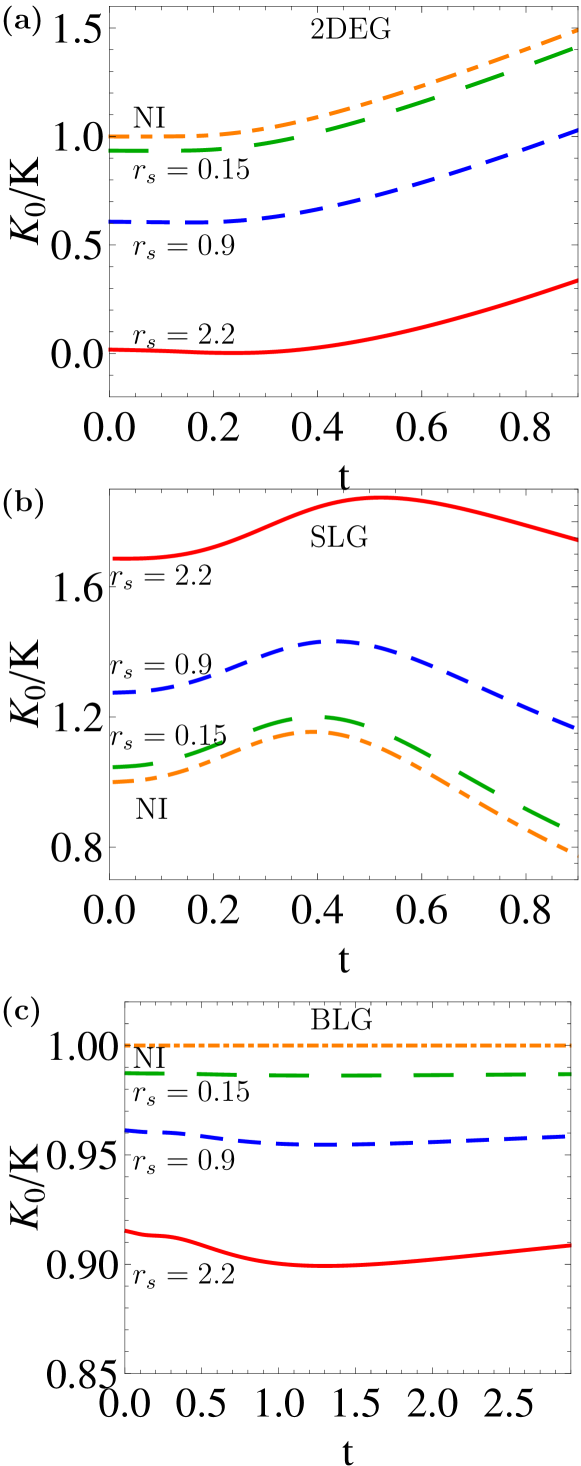
Figure 9: (color online) Calculated $K_{0}/K$ for the 2D, MLG, and BLG systems as a function of $t$ for a few values of $r_{s}$.

V Discussion and Conclusion

In this work, we have calculated the finite temperature compressibility of graphene and ordinary 2D semiconductor systems within the Hartree-Fock approximation. We present both analytical and numerical results of $K_{0}/K$ as a function of temperature, the dimensionless interaction parameter $r_{s}$, and density. We find that the calculated temperature dependent compressibility is non-monotonic in both graphene and 2D semiconductor systems. In monolayer graphene, the inverse compressibility $K^{-1}$ increases with temperature at low temperatures and decreases at high temperatures, reaching a maximum value at an intermediate temperature. This non-monotonicity arises entirely from the behavior of the non-interacting graphene compressibility. The temperature dependent inverse compressibility in 2D semiconductor systems decreases with temperature at low temperatures and increases at high temperatures. In BLG the inverse compressibility decreases as temperature increases at low temperatures, but it approaches a value which is less than the non-interacting value at high temperatures. The leading order temperature correction to the inverse compressibility $K^{-1}$ in HFA for both graphene and 2D semiconductor systems is $t^{2}\ln t$. Our analytic results are in agreement with our numerical results both at low and at high temperatures.

Our use of the Hartree-Fock approximation is not a particularly restrictive approximation for the theory of the electronic compressibility since it is well-known that Hartree-Fock theory works well for the calculation of the compressibility and its density dependence, at least at $T=0$. The Hartree-Fock approximation gives results numerically very close to the full dynamical RPA for the 2D compressibility at $T=0$ Das Sarma et al. (2009), and the Hartree-Fock compressibility results are in good agreement with the compressibility measurements for 2D semiconductorsEisenstein et al. (1994) and grapheneHwang et al. (2007). In fact, the Hartree-Fock approximation for 2D semiconductors is in better quantitative agreement with the density dependence of the measured compressibilityEisenstein et al. (1994) than the corresponding RPA theory as long as the strict 2D approximation is used since the finite width corrections for the realistic 2D semiconductors tend to cancel out the correlation corrections neglected in the HFA. In any case, we consider the HFA as the first step necessary for understanding the temperature dependent 2D compressibility in interacting electron systems, and only future work, particularly experiments comparing with our predictions, can establish the necessity of improved theoretical treatments involving dynamical correlations neglected in the HFA.

Our main finding that the temperature dependence of compressibility is much stronger in 2D systems than in graphene is consistent with existing experimental results. In particular, our results of Sec. II agree well with the experimental study of Shapira et al.,Shapira et al. (1996) on 2D GaAs holes who discovered substantial temperature dependence in the 2D hole compressibility in the $1-100$ K temperature regime with the experimental data showing reasonable qualitative agreement with our theoretical HFA results presented in Sec. IID. Detailed quantitative comparison with the experimental data of Shapira et al.,Shapira et al. (1996) is not particularly meaningful (and is not attempted) because of a number of reasons including our use of the exchange-only Hartree-Fock approximation, our neglect of the finite thickness of the 2D semiconductor structures which is often important for quantitative considerations, our neglect of disorder effects which are certainly important at lower carrier densities, and the lack of information about some essential experimental parameters (e.g., depletion charge density).

In addition to the experimental study of the temperature dependent 2D hole compressibility by Shapira et al., Shapira et al. (1996) discussed above, there have been several low-density studies of the temperature dependence of the compressibility in both electron and hole 2D systemsEisenstein et al. (1992, 1994); Shapira et al. (1996) carried out in the context of 2D MIT (i.e., disorder-induced density-tuned localization of 2D semiconductor systems). As we discussed in Sec. II, these low-density experimental investigations should be revisited in light of our current work demonstrating the importance of the temperature dependence of $K_{0}/K$ in the low carrier density regime by virtue of the dimensionless temperature $T/T_{F}$ being large precisely in the low-density regime (where disorder effects are also strong) since $T_{F}\propto n$ in 2D systems. Unfortunately, temperature, disorder, and interaction effects are all strong in the low density regime, making any quantitatively reliable theoretical work essentially impossible in the low carrier density regime, and our work establishes the importance of finite temperature effects on the compressibility in the low carrier density regime. In particular, the density inhomogeneity and puddle formation that happens at low carrier density Yamaguchi et al. (2008); Allison et al. (2006) due to the failure of screening would very much complicate the observation of the low-density (and low-temperature) features in the compressibility predicted in our theory unless one uses extremely high-quality samples with very low disorder. Recently, there has been a theoretical investigation Abergel et al. (2011) of the effect of disorder on low-density graphene compressibility clearly establishing the importance of disorder in low-density compressibility.

Since the Fermi temperature $T_{F}$ goes as $T_{F}$(in K)$=4.2\tilde{n}$ (2D GaAs electrons); $0.74\tilde{n}$ (2D GaAs holes); $136\sqrt{\tilde{n}}$ (monolayer graphene); $4.2\tilde{n}$ (bilayer graphene), where $\tilde{n}\equiv n/10^{10}$ is the carrier density measured in the units of $10^{10}$ cm^-2, it is obvious that the quantitative effect of finite temperature, even at low carrier densities, is by far the strongest (weakest) in 2D GaAs holes (monolayer graphene), which is consistent with experimental observations. Since disorder effects become important for $n\lesssim n_{i}$, where $n_{i}$ is the background random charged impurity density in the environment, the low density regime associated with large $T/T_{F}$ values becomes even more challenging to achieve in the laboratory experiments on graphene. We expect our predicted temperature dependence to manifest in graphene compressibility in room temperature experiments in very high-mobility samples where $T/T_{F}\sim 1$ values may be achievable.

An important relevant question for our theory is: what is the most suitable system for the experimental observation of our theoretical predictions? Obviously, our predicted high-temperature behavior, where the theory is in very firm ground since the exchange energy is likely to be the exact leading-order many-body correction to the non-interacting compressibility in the high-temperature limit, should be valid for all systems and should be observable in 2D semiconductors (both electrons and holes) rather easily by measuring the compressibility for $T=10-200$ K for electron (hole) densities$\sim 10^{10}-10^{11}$ cm^-2 so that $T>r_{s}^{2}T_{F}$ condition is satisfied. Given that $T_{F}^{h}<T_{F}^{e}$ at the same density, the high-temperature behavior is much more easily observable in 2D GaAs holes, and has, in fact, already been observed at least in one experimental study in 2D holesShapira et al. (1996). While 2D GaAs holes are the obvious ideal candidates for observing our predicted high-temperature compressibility behavior, monolayer graphene may turn out to be not particularly well-suited for the temperature-dependent compressibility studies because of its very high relative Fermi-temperature ($T_{F}^{MLG}\sim 1350$ K for a doping density of $10^{12}$ cm^-2) and its relatively weak temperature dependence. Obviously, the condition for observing the high-temperature behavior of compressibility is the ability to reach $T\gtrsim T_{F}$ which necessitates lower Fermi temperatures. By contrast, the low-$T$ behavior associated with the $T^{2}\ln T$ term in the compressibility may be better observed in a system with a relatively high value of $T_{F}$ so that the regime $T/T_{F}<1$ can be explored over a fairly broad range of temperature with the temperature $t_{m}$ not being too low. Thus, very high mobility n-GaAs heterostructures or quantum wells with $n\sim 2\times 10^{10}$ cm^-2 so that $T_{F}\sim 8.3$ K (and $T_{m}\sim 3$ K) may be the ideal system to search for our predicted shallow minimum in $K_{0}/K$. One serious problem is that the minimum may be too shallow to be uniquely determined experimentally.

Finally, we discuss our very interesting analytical finding of the non-monotonicity in graphene inverse compressibility associated with the $T^{2}\ln T$ correction we obtain analytically (and verify numerically). Although this would not be an easy effect to detect experimentally because of its quantitative weakness (and became the subleading correction goes as $T^{2}$ and thus the ratio of the two, $\ln(T/T_{F})$, is always challenging to observe in experiments even under the best of circumstances), it is nevertheless interesting to discuss its origin and its robustness beyond our approximation scheme. Our results are exact within the Hartree-Fock approximation scheme, and there is no doubt that the exchange self-energy contributes a $T^{2}\ln T$ leading-order contribution to the inverse compressibility. The first question is whether this is intrinsically a dimensionality effect occurring only in two dimensions. We have therefore carried out the corresponding analytical calculations for the 3D temperature-dependent compressibility (presented in the Appendix A of this paper), finding that $K_{0}/K$ has a $T^{2}\ln T$ contribution in three dimensions also. Thus, it appears that the interesting non-monotonicity associated with the $T^{2}\ln T$ correction is a results of the Hartree-Fock approximation arising from the exchange self-energy diagram, and is not intrinsically a two-dimensional effect.

We have investigated this question by calculating the interacting compressibility in the screened Hartree-Fock approximation (sometimes also called static RPA) for the 2D system, where the bare Coulomb interaction ‘$V$’ appearing in the exchange self-energy is screened by the static RPA dielectric function. (These results are shown in Appendix B.) The screened HFA (Appendix B) or static RPA does not contain the $T^{2}\ln T$ term in the finite temperature inverse compressibility, but is not a reliable approximation at all since at $T=0$ it predicts that $K_{0}/K$ should be always positive for all values of $r_{s}$ in clear disagreement with experimental findingEisenstein et al. (1992, 1994). Thus the absence of the $T^{2}\ln T$ term in the screened HF approximation cannot be taken seriously since the corresponding $T=0$ result is in qualitative disagreement with experimental results. It is interesting to speculate whether the $T^{2}\ln T$ term survives higher-order diagrams associated with dynamical correlation effects, and this remains a challenge for the future. Although it is fairly straightforward to calculate the compressibility including correlation effects at $T=0$ — for example, the ring-diagram contributions to the compressibility can be exactly calculated at $T=0$  Das Sarma et al. (2009) — it is a formidable challenge, both numerically and analytically, to extend to the corresponding ring diagram calculations of interacting compressibility to finite temperatures. We have studied this question carefully and have been able to show that there is definitely a $T^{2}$ term in $K_{0}/K$ arising from the infinite series of the ring diagrams, but we still do not know whether the $T^{2}\ln T$ term of the exchange self-energy is exactly canceled by the dynamical effects arising from the infinite ring diagram series. Although the effect of the $(T/T_{F})^{2}\ln(T/T_{F})$ term matters only at low temperatures and low densities, where disorder effects dominate making it difficult to observe the log term experimentally, it is nevertheless important to establish whether this non-monotonicity associated with $T^{2}\ln T$ survives higher-order correlation terms in the theory. We leave this as an unanswered theoretical question for the future. A direct experimental observation of the $T^{2}\ln T$ term in the low-temperature inverse compressibility of 2D electrons or holes will go a long way in settling this important question.

To summarize, our goal of this paper is to understand the temperature dependence of compressibility in a high density homogeneous system where the interaction effect is not too strong and HFA is valid. At very low density, disorder effects are of particular importance and the system may be highly inhomogeneous due to the formation of electron-hole puddlesIlani et al. (2000); Dultz et al. ; Shi and Xie (2002); Das Sarma et al. (2011); Gao ; Abergel et al. (2011, ); Yamaguchi et al. (2008); Allison et al. (2006); Hwang and Das Sarma (2010); Li et al. (2011); Rossi and Das Sarma (2008), which are not included in our theory. Our main result is that temperature effects in the compressibility could be quite important at higher temperatures.

Appendix A Hartree-Fock compressibility in 3DEG

In this Appendix, we provide the corresponding finite temperature Hartree-Fock compressibility for a standard three dimensional electron gas (3DEG). For 3DEG, the bare Coulomb interaction $V(q)=\dfrac{4\pi e^{2}}{\kappa q^{2}}$, where $\kappa$ is the background dielectric constant. We assume the total degeneracy $g=2$ in the calculation.

The finite temperature exchange energy of 3DEG is given by

$$\begin{array}[]{l l l l l }\Sigma_{\text{ex}}(k)&=&-\int\frac{d^{3}k^{\prime}}{(2\pi)^{3}}V(|k-k^{\prime}|)n_{F}(\xi_{k^{\prime}})\\ \\ &=&-\dfrac{e^{2}k}{\pi\kappa}\int_{0}^{1}\text{d}x\ln\left(\dfrac{1+x}{1-x}\right)\Big{[}\dfrac{x}{e^{\beta(\epsilon_{k}x^{2}-\mu_{0})}+1}\\ \\ &+&\dfrac{1/x^{3}}{e^{\beta(\epsilon_{k}/x^{2}-\mu_{0})}+1}\Big{]}\end{array}$$ (65)

where $\beta=1/k_{B}T$, $\epsilon_{k}=k^{2}/2m$, $m$ is the effective mass, and $\mu_{0}$ is the finite temperature chemical potential without exchange energy. The non-interacting chemical potential, $\mu_{0}$, is obtained by solving the following self-consistent equation,

$$n=\dfrac{k_{F}^{3}}{\pi^{2}}\int_{0}^{\infty}\text{d}x\frac{x^{2}}{\exp(\frac{x^{2}-\tilde{\mu_{0}}}{t})+1}$$ (66)

where $\tilde{\mu_{0}}=\mu_{0}/E_{F}$, $t=T/T_{F}$ and $n=\dfrac{k_{F}^{3}}{3\pi^{2}}$ for 3DEG. There is no explicit analytical formula for the finite temperature chemical potential in 3DEG. But at very low temperatures ($t\ll 1$), the asymptotic form of the non-interacting chemical potential is given by

$$\begin{array}[]{l l}\mu_{0}\approx E_{F}\left(1-\dfrac{\pi^{2}t^{2}}{12}\right)\end{array}$$ (68)

The HFA chemical potential, $\mu$, can be calculated by including the exchange energy for $k=k_{F}$, i.e.,

$$\mu=\mu_{0}(T)+\Sigma_{ex}(k_{F},T).$$ (69)

Then, the normalized chemical potential $\tilde{\mu}=\mu/E_{F}$ can be expressed

$$\tilde{\mu}=\tilde{\mu_{0}}-\frac{2\alpha}{\pi}\int_{0}^{1}\text{d}x\ln\left(\dfrac{1+x}{1-x}\right)\left[\frac{x}{e^{(x^{2}-\tilde{\mu_{0}})/t}+1}\right.$$

$$\left.+\frac{1/x^{3}}{e^{(1/x^{2}-\tilde{\mu_{0}})/t}+1}\right],$$ (70)

where $\alpha=({4}/{9\pi})^{1/3}r_{s}$ with the dimensionless parameter $r_{s}=(3/4\pi n)^{1/3}(me^{2}/\kappa)$, and

$$\tilde{\mu_{0}}=1-\frac{\pi^{2}t^{2}}{12}.$$ (71)

By differentiating Eq. (69) with respect to $n$ and using $k_{F}^{3}=3\pi^{2}n$, the corresponding non-interacting compressibility of 3DEG is given by

$$\frac{1}{n^{2}K_{0}}=\frac{dE_{F}}{dn}=\frac{\pi^{2}}{mk_{F}}$$ (72)

$$\frac{1}{n^{2}K_{ni}}=\frac{d\mu_{0}}{dn}=\frac{h_{3}(t)}{K_{0}},$$ (73)

where $K_{0}$ and $K_{ni}$ are the zero temperature and the finite temperature non-interacting compressibility, respectively, and $h_{3}(t)=1+\dfrac{\pi^{2}t^{2}}{12}$.

The finite temperature inverse compressibility $K_{0}/K$ within HFA is given by

$$\frac{K_{0}}{K}=h_{3}(t) - \dfrac{\alpha}{\pi}\int_{0}^{1}\text{d}x\ln\left(\dfrac{1+x}{1-x}\right)\left[\frac{x}{e^{(x^{2}-\tilde{\mu_{0}})/t}+1}+\frac{1/x^{3}}{e^{(1/x^{2}-\tilde{\mu_{0}})/t}+1}\right]$$ (74)

$$+ \dfrac{\alpha}{2\pi t}\int_{0}^{1}\text{d}x\ln\left(\dfrac{1+x}{1-x}\right)\left[\frac{x(x^{2}-h(t))}{\cosh^{2}\frac{(x^{2}-\tilde{\mu_{0}})}{2t}}+\frac{\frac{1}{x^{3}}(\frac{1}{x^{2}}-h(t))}{\cosh^{2}\frac{(1/x^{2}-\tilde{\mu_{0}})}{2t}}\right].$$

At zero temperature $T=0$, we have

$$\frac{K_{0}}{K}=1-\frac{\alpha}{\pi}=1-\frac{1}{\pi}\sqrt[3]{\dfrac{4}{9\pi}}r_{s}.$$ (75)

The HF chemical potential and the compressibility in the low temperature limit $t\ll 1$ can be calculated by expanding the logarithmic function near $x=1$. Then the chemical potential in Eq. (70) becomes

$$\tilde{\mu}=\tilde{\mu_{0}}-\frac{2}{\pi}\sqrt[3]{\dfrac{4}{9\pi}}r_{s}\left[1+\frac{\pi^{2}t^{2}}{24}(A_{3}+\text{ln}t)\right],$$ (76)

where $A_{3}=1-\gamma+\text{ln}\Big{(}\dfrac{\pi}{8}\Big{)}$ (where $\gamma$ is Euler’s constant, with numerical value $\simeq 0.577216$.). Finally we find that the low temperature 3D inverse compressibility within HFA as

$$\dfrac{K_{0}}{K}\Big{|}_{t\rightarrow 0} = 1+\dfrac{\pi^{2}t^{2}}{12}-\sqrt[3]{\dfrac{4}{9\pi^{4}}}r_{s}\left[1\right.$$ (77)

$$+ \left.0.136\pi^{2}t^{2}+\dfrac{1}{8}\pi^{2}t^{2}\text{ }\ln(\dfrac{\pi t}{8})\right].$$

The asymptotic behavior of high temperature compressibility is obtained by approximating the Fermi-Dirac distribution function by the classical Boltzmann function. In the high temperature regime $t\rightarrow\infty$, the normalized chemical potential within HFA becomes

$$\tilde{\mu}\Big{|}_{t\rightarrow\infty}=t\ln\left(\frac{4}{3\sqrt{\pi}t^{3/2}}\right)-\frac{8}{3t}\sqrt[3]{\frac{4}{9\pi^{4}}}r_{s},$$ (78)

and the corresponding high temperature inverse compressibility is calculated as

$$\dfrac{K_{0}}{K}\Big{|}_{t\rightarrow\infty}=\frac{3t}{2}-\frac{4}{t}\sqrt[3]{\frac{4}{9\pi^{4}}}r_{s},$$ (79)

which agrees with the non-interacting high-temperature classical result.

Appendix B Screened 2D Hartree-Fock compressibility

We provide the screened Hartree-Fock compressibility (sometimes also called static RPA) for the 2D system, where the bare Coulomb interaction ‘$V$’ appearing in the exchange self-energy is screened by the static RPA dielectric function.

The self-energy with the finite temperature static RPA dielectric function is given by

$$\Sigma_{\text{self}}(k_{F})=-\int\frac{d^{2}q}{(2\pi)^{2}}\frac{V(q)}{\epsilon(q,T)}n_{F}\left(\xi_{q-k_{F}}\right)$$ (80)

where $V(q)=\dfrac{2\pi e^{2}}{\kappa q}$, $n_{F}\left(\xi_{q-k_{F}}\right)$ is the Fermi distribution function. The static RPA dielectric function $\epsilon\left(q,T\right)$ is given by Das Sarma et al. (2011)

$$\epsilon\left(q,T\right)=1+V(q)\Pi(q,T)=1+\frac{q_{s}(q,T)}{q}$$ (81)

where $\Pi(q,T)$ is the finite temperature static polarization function and $q_{s}=2\pi e^{2}\Pi(q,T)/\kappa$ is the momentum dependent screening wave vector Das Sarma et al. (2011). At low temperatures ($T\ll T_{F}$) the 2D polarizability becomes Das Sarma et al. (2011),

$$\Pi(q,T)\approx\frac{m}{\pi}\left(1-e^{-T_{F}/T}\right),$$ (82)

and its asymptotic form at high temperatures ($T\gg T_{F}$) becomesDas Sarma et al. (2011)

$$\Pi(q,T)\approx\frac{m}{\pi}\frac{T_{F}}{T}.$$ (83)

The finite temperature chemical potential within static RPA, $\mu(T)$, can be calculated by including the self-energy of Eq. (80), i.e.,

$$\mu(T)=\mu_{0}(T)+\Sigma_{\text{self}}(k_{F},T).$$ (84)

At zero temperature ($T=0$), the non-interacting part of chemical potential is the Fermi energy $\mu=E_{F}$. For $r_{s}\ll 1$, the chemical potential approaches the non-interacting value, which has been discussed in Sec. II. For interacting 2D systems the self-energy within screened HFA has the asymptotic form (with $g_{s}=2$ and $g_{v}=1$) for $r_{s}\gg 1$,

$$\Sigma_{\text{self}}(k_{F},T=0)\Big{|}_{r_{s}\gg 1}=-\frac{\pi n}{2m}.$$ (85)

Differentiating Eq. 85 with respect to $n$ and using the relation $k_{F}^{2}=2\pi n$, we get the zero temperature inverse compressibility within the screened HFA

$$\frac{K_{0}}{K(T=0)}\Big{|}_{r_{s}\gg 1}=\frac{1}{2}.$$ (86)

Since $K_{0}$ is a positive value we have the positive compressibility even for $r_{s}\gg 1$, which clearly disagrees with both the HF results and experimentsEisenstein et al. (1992, 1994).

With Eqs. (80)–(82), we find the asymptotic form of the self-energy at low temperatures ($T\ll T_{F}$) and for $r_{s}\gg 1$

$$\Sigma_{\text{self}}(k_{F},T)\Big{|}_{r_{s}\gg 1}=-\frac{\pi n}{2m}+O(e^{-T_{F}/T}).$$ (87)

We find that the leading order temperature dependent term in the self energy is exponentially suppressed. Consequently, the temperature dependent inverse compressibility at low temperatures becomes

$$\frac{K_{0}}{K(T\ll T_{F})}\Big{|}_{r_{s}\gg 1}\approx\frac{1}{2}+O(e^{-T_{F}/T}).$$ (88)

At high temperatures ($T\gg T_{F}$), the inverse compressibility calculated within the static RPA approaches the HFA results given in Eq. (18) because the non-interacting kinetic energy dominates.

References

- Eisenstein et al. (1992) J. P. Eisenstein, L. N. Pfeiffer, and K. W. West, Phys. Rev. Lett. 68, 674 (1992).
- Eisenstein et al. (1994) J. P. Eisenstein, L. N. Pfeiffer, and K. W. West, Phys. Rev. B 50, 1760 (1994).
- Dultz and Jiang (2000) S. C. Dultz and H. W. Jiang, Phys. Rev. Lett. 84, 4689 (2000).
- Ilani et al. (2000) S. Ilani, A. Yacoby, D. Mahalu, and H. Shtrikman, Phys. Rev. Lett. 84, 3133 (2000).
- (5) S. C. Dultz, B. Alavi, and H. W. Jiang, arXiv:cond-mat/0210584 (2002).
- Das Sarma and Hwang (2005) S. Das Sarma and E. H. Hwang, Solid State Commun. 135, 579 (2005).
- Shi and Xie (2002) J. Shi and X. C. Xie, Phys. Rev. Lett. 88, 086401 (2002).
- Das Sarma et al. (2011) S. Das Sarma, S. Adam, E. H. Hwang, and E. Rossi, Rev. Mod. Phys. 83, 407 (2011).
- Pines and Nozieres (1966) D. Pines and P. Nozieres, The Theory of Quantum Liquids (Benjamin, Reading, Mass., 1966).
- Mahan (2000) G. D. Mahan, Many-Particle Physics, Third Edition (Kluwer Academic/Plenum Pulishers, New York, USA, 2000).
- (11) X. P. A. Gao, unpublished and private communication.
- Martin et al. (2008) J. Martin, N. Akerman, G. Ulbricht, T. Lohmann, J. H. Smet, K. V. Klitzing, and A. Yacoby, Nat. Phys. 4, 144 (2008).
- Hwang et al. (2007) E. H. Hwang, B. Y.-K. Hu, and S. Das Sarma, Phys. Rev. Lett. 99, 226801 (2007).
- Barlas et al. (2007) Y. Barlas, T. Pereg-Barnea, M. Polini, R. Asgari, and A. H. MacDonald, Phys. Rev. Lett. 98, 236601 (2007).
- Shapira et al. (1996) S. Shapira, U. Sivan, P. M. Solomon, E. Buchstab, M. Tischler, and G. Ben Yoseph, Phys. Rev. Lett. 77, 3181 (1996).
- Millard et al. (1997) I. S. Millard, N. K. Patel, C. L. Foden, E. H. Linfield, M. Y. Simmons, D. A. Ritchie, and M. Pepper, Phys. Rev. B 55, 6715 (1997).
- Abergel et al. (2011) D. S. L. Abergel, E. H. Hwang, and S. Das Sarma, Phys. Rev. B 83, 085429 (2011).
- Hwang and Das Sarma (2009) E. H. Hwang and S. Das Sarma, Phys. Rev. B 79, 165404 (2009).
- Kusminskiy et al. (2008) S. V. Kusminskiy, J. Nilsson, D. K. Campbell, and A. H. Castro Neto, Phys. Rev. Lett. 100, 106805 (2008).
- Borghi et al. (2010) G. Borghi, M. Polini, R. Asgari, and A. H. MacDonald, Phys. Rev. B 82, 155403 (2010).
- (21) D. S. L. Abergel, H. Min, E. H. Hwang, and S. D. Sarma, Phys. Rev. B 84, 195423 (2011).
- Sensarma et al. (2011) R. Sensarma, E. H. Hwang, and S. Das Sarma, Phys. Rev. B 84, 041408 (2011).
- Henriksen and Eisenstein (2010) E. A. Henriksen and J. P. Eisenstein, Phys. Rev. B 82, 041412 (2010).
- (24) A. F. Young, C. R. Dean, I. Meric, S. Sorgenfrei, H. Ren, K. Watanabe, T. Taniguchi, J. Hone, K. L. Shepard, and P. Kim, arXiv:1004.5556v2 (2010).
- Martin et al. (2010) J. Martin, B. E. Feldman, R. T. Weitz, M. T. Allen, and A. Yacoby, Phys. Rev. Lett. 105, 256806 (2010).
- Das Sarma et al. (2009) S. Das Sarma, E. H. Hwang, and Q. Li, Phys. Rev. B 80, 121303(R) (2009).
- Yamaguchi et al. (2008) M. Yamaguchi, S. Nomura, T. Maruyama, S. Miyashita, Y. Hirayama, H. Tamura, and T. Akazaki, Phys. Rev. Lett. 101, 207401 (2008).
- Allison et al. (2006) G. Allison, E. A. Galaktionov, A. K. Savchenko, S. S. Safonov, M. M. Fogler, M. Y. Simmons, and D. A. Ritchie, Phys. Rev. Lett. 96, 216407 (2006).
- Hwang and Das Sarma (2010) E. H. Hwang and S. Das Sarma, Phys. Rev. B 82, 081409 (2010).
- Li et al. (2011) Q. Li, E. H. Hwang, and S. Das Sarma, Phys. Rev. B 84, 115442 (2011).
- Rossi and Das Sarma (2008) E. Rossi and S. Das Sarma, Phys. Rev. Lett. 101, 166803 (2008).