Convergence analysis of a high-order Nyström integral-equation method for surface scattering problems

Abstract

In this paper we present a convergence analysis for the Nyström method proposed in [Jour. Comput. Phys. 169 pp. 2921-2934, 2001] for the solution of the combined boundary integral equation formulations of sound-soft acoustic scattering problems in three-dimensional space. This fast and efficient scheme combines FFT techniques and a polar change of variables that cancels out the kernel singularity. We establish the stability of the algorithms in the $L^{2}$ norm and we derive convergence estimates in both the $L^{2}$ and $L^{\infty}$ norms. In particular, our analysis establishes theoretically the previously observed super-algebraic convergence of the method in cases in which the right-hand side is smooth.

Key words: Acoustic Scattering, Boundary Integral Equations, Nyström methods, FFT
MSC: 65N38, 65N35, 65T40

1 Introduction

In this paper we present a full convergence analysis of the high-order Nyström method introduced by Bruno and Kunyansky in [6, 7] for boundary integral equations (BIE) related to the scattering of time-harmonic acoustic waves by arbitrary (smooth) surfaces in three-dimensional space. In particular, our analysis establishes theoretically the previously observed super-algebraic convergence of the method for smooth right-hand sides. To the best of the authors’ knowledge, this proof constitutes one of the few instances of analysis of a Nyström type method for a boundary integral equation in three dimensions.

As is well known, Galerkin methods for BIE of the first kind have enjoyed thorough theoretical analyses since their inception—on the basis of ellipticity properties and discrete Fredholm theory. Compactness arguments can also be used to establish convergence of Galerkin methods for equations of the second kind. Few results exist, on the other hand, concerning convergence for three-dimensional BIE collocation methods—in which finite-element bases are used for approximation, but testing relies on point sampling. We refer to the excellent text-book [3, Chapter 9] for a brief introduction on this topic.

This state of affairs has led to the widespread perception that, being even more “discrete” than collocation schemes, Nyström methods for BIEs of the second kind with weakly singular kernels could not be easily analyzed. This paper will hopefully help dispell this view and lend additional credibility to Nyström methods—whose qualities can be very attractive in practice [6].

One of the main difficulties in the design of three-dimensional integral solvers concerns development of high-quality quadrature rules for approximation of singular integral terms. Wienert [24] constructed a singular integration rule on the basis of spherical-harmonic transforms for surfaces for which a diffeomorphism to the sphere can be constructed, (see also [12, Section 3.6]). A Galerkin version of this approach was introduced and analyzed in [16] where, in particular, the superalgebraic convergence of the method was established. Reference [15] presents a collocation method, with corresponding analysis, for the Laplace equation, which shares the good convergence properties of the method by Wienert but which again is limited to surfaces for which a smooth mapping from the sphere is available. We emphasize that such limitations, which are highly restrictive in practice, are not imposed by the Nyström method studied in this paper.

We thus consider the numerical method [6] for the second-kind combined field integral equation associated to the problem of sound-soft scattering by a three dimensional obstacle with smooth boundary $S$. The method relies on a series of geometric constructions: 1) Representation of the surface by means of a set of $J$ overlapping smooth charts (parametrizations); 2) A smooth partition of unity subordinated to these charts which decomposes both the overall integral operators as well as the solution of the BIE as the sum of contributions defined on the parametrized patches; 3) A family of floating smooth cut-off functions $\eta_{\delta}:S\times S\to\mathbb{R}$ (see (2.10) below) that is used to isolate the singularity of the kernel function, and thus produces a splitting of the integral operator of the form $K=K_{\mathrm{reg},\delta}+K_{\mathrm{sing},\delta}$—whereby the regular operator is an integral operator with a smooth kernel, and the singular part which enjoys a reduced domain of integration but contains the weak singularity of the integral kernel.

The Nyström method under consideration is based on approximation of the integral operator by a quadrature rule which treats the regular and singular parts $K_{\mathrm{reg},\delta}$ and $K_{\mathrm{sing},\delta}$ separately. The $J$ local charts mentioned above are used to push forward $J$ uniform grids from the unit square to the surface; these grids are used for both, approximation and integration. The quadrature rule used for the regular operator $K_{\mathrm{reg},\delta}$ is based on application of the two-dimensional trapezoidal rule in the parameter space $[0,1]\times[0,1]$ for each one of the $J$ parametric domains: since the corresponding integrands are smooth with compact support strictly contained in the unit square, these trapezoidal quadratures give rise to super-algebraically accurate approximations. For the singular part, a change of variables to polar coordinates around each integration point is applied. This procedure results in a smooth integrand to which, upon necessary Fourier-based interpolations, the trapezoidal rule is applied for radial and angular integration—once again yielding super-algebraically accurate approximations.

As a result of these constructions we obtain an algorithm that evaluates the action of an approximating discrete operator on a continuous function, using only the values of the function on the selected quadrature points.

Our theoretical treatment relies on use of both existing and new analytical tools. In a first key step of the analysis the problem is re-expressed as a system of integral equations in a space of periodic functions. This is accomplished by means of yet another set of local cut-off functions, whose presence does not affect the actual numerical scheme. The use of periodic Sobolev spaces allows us to take full advantage of numerous results for approximation of Fourier series and interpolation operators [22], as well as the theory of collective compact operators by Anselone [2]. Recasting the numerical scheme of quadrature type as a discretization method in $L^{2}$-type (Sobolev) spaces gives rise to a number of difficulties. In particular, for the sake of the analysis we introduce Fourier projection operators, bi-periodic trigonometric interpolation operators, and a discrete operator [10] that produces a linear combination of Dirac delta distributions on a uniform grid from a smooth function input. The convergence analysis for the operators arising from the regular part of the original boundary integral operator follows the lines of the theory [10, 14] on periodic integral equations in one variable. The final (rather technical) element of our convergence proof is a detailed analysis of the integration error arising from the numerical polar coordinate integration algorithm for products of smooth functions, “shrinking” floating cut-off functions and bi-variate trigonometric polynomials, in terms of Sobolev norms of the latter polynomials.

We point out that, for efficiency, a variety of acceleration techniques were used in [6, 7] in conjunction with the Nyström algorithm we consider. Some of these algorithmic components have been taken into account in our analysis. In the formulation considered in the present paper, for example, the computation of the singular part requires the evaluation of bivariate trigonometric polynomials that approximate the unknown at points on a polar grid. A deliberate choice of the radial quadrature nodes for this integral makes it possible to reduce this process to 1–dimensional trigonometric interpolation problems (see section 2.3 and Figure 3 below) on the horizontal and vertical lines of the grid. In [6], such trigonometric polynomials are then approximated by means of piecewise Hermite interpolation on dyadic grids, which can be evaluated much more rapidly than the either of the underlying trigonometric polynomials. We have analyzed the effect of these additional approximations on the full convergence of the Nyström method. The corresponding results can be found in Appendix B; briefly, upon correct parameter selections, the resulting (more efficient) method retains the super-algebraic convergence of the original approach. Additional, more sophisticated acceleration techniques which, based on use of equivalent sources and Fast Fourier Transforms, provide a means to reduce the solution cost for high-frequency problems (but on which the Nyström method itself does not depend, and whose use is not advantageous for problems of lower frequencies) were introduced in [6]. The impact of such equivalent-source acceleration methods on convergence are not considered either in the present paper or in the Appendix B of this paper.

This paper is structured as follows. In Section 2 we describe, in a compact form, the Nyström method under consideration, and we state the main convergence results of this paper. In Section 3 we then recast both the continuous and discrete problems as systems of equations in spaces of biperiodic functions, we derive bounds, on various norms, of the main continuous integral operators in our periodic formulation, we establish unique solvability of the continuous system of periodic integral equations as well as the equivalence of this system to the original BIE, and, finally, we state the main approximation results in the biperiodic frame: norm convergence of the discrete operators to the continuous ones together with corresponding error estimates. In Section 4 we present key estimates on the singular operators that appear in the biperiodic formulation, and in Section 5, in turn, we provide the proofs of the main results stated in Section 3 and Section 2—in that order. Appendix A is devoted to the Sobolev error analysis mentioned above for the polar-integration of products of smooth functions, cut-offs and trigonometric polynomials. Finally, in Appendix B we describe and analyze a slight variant of the numerical method, where one of the interpolation processes is substituted by polynomial interpolation.

We conclude our introduction with two remarks concerning notation.

Remark 1.1

To make a clearly visible distinction between points on the surface $S$ and coordinates for their parametrization, we use boldface letters (e.g. ${\bf r}$) for points on the scattering surface $S\subset\mathbb{R}^{3}$, and underlined letters (such as $\underline{u}$) for points in $\mathbb{R}^{2}$. The coordinates of such points will be denoted according to $\underline{u}=(u_{1},u_{2})$.

Remark 1.2

Throughout this paper the letter $C$ denotes a positive constant independent of the parameters $h$ and $\delta$ and any other variable quantities appearing in the equation. When necessary a subscripted letter $C$ is used—either to avoid confusion or to explicitly signify dependence on parameters other than $h$ and $\delta$.

2 The Nyström method

2.1 The Boundary Integral Equation

We consider the problem of time-harmonic acoustic scattering by a sound-soft obstacle with smooth boundary $S$ in three-dimensional space:

$$\left[\begin{array}[]{rcll}\Delta U+\kappa^{2}U&=&0&\mbox{in $\mathrm{ext}(S)$},\\[4.73611pt] U&=&-U^{\rm inc}&\mbox{on $S$},\\[4.73611pt] \partial_{r}U-{\rm i}\kappa U&=&o(r^{-1})&\mbox{as }r\to\infty.\end{array}\right.$$ (2.1)

Here $\kappa>0$ is the wave number, $U^{\rm inc}$ is the incident wave, $r:=|{\bf x}|$ and $\partial_{r}$ denotes the radial derivative. Letting $\Phi_{\kappa}$ denote the fundamental solution of the Helmholtz equation,

$$\Phi_{\kappa}({\bf r},{\bf r}^{\prime}):=\frac{\exp({\rm i}\kappa|{\bf r}-{\bf r}^{\prime}|)}{4\pi\,|{\bf r}-{\bf r}^{\prime}|},$$

then the solution $U$ of (2.1) can be expressed as the combined (or Brakhage-Werner [4]) potential

$$U({\bf r})=\int_{S}\frac{\partial\Phi_{\kappa}({\bf r},{\bf r}^{\prime})}{\partial\bm{\nu}({\bf r}^{\prime})}\psi({\bf r}^{\prime}){\rm d}{\bf r}^{\prime}-{\rm i}\eta\int_{S}\Phi_{\kappa}({\bf r},{\bf r}^{\prime})\psi({\bf r}^{\prime}){\rm d}{\bf r}^{\prime},$$

where $\frac{\partial}{\partial\bm{\nu}}$ denotes the outward normal derivative on $S$ and $\eta>0$ is a coupling parameter. The density $\psi$ is the unique solution of the integral equation

$${\textstyle\frac{1}{2}}\psi({\bf r})+A\psi({\bf r})=-U^{\rm inc}({\bf r})\qquad\forall{\bf r}\in S,$$ (2.2)

where

$$A\psi({\bf r})=\int_{S}K({\bf r},{\bf r}^{\prime})\psi({\bf r}^{\prime})\,{\rm d}{\bf r}^{\prime}:=\int_{S}\Big{(}\frac{\partial\Phi_{\kappa}({\bf r},{\bf r}^{\prime})}{\partial\bm{\nu}({\bf r}^{\prime})}-{\rm i}{\eta}\Phi_{\kappa}({\bf r},{\bf r}^{\prime})\Big{)}\psi({\bf r}^{\prime}){\rm d}{\bf r}^{\prime}.$$ (2.3)

Various choices of the coupling parameter $\eta$ have been proposed for accuracy and numerical efficiency; see e.g. [8, 11, 13, 6]. Note that the kernel $K$ can be expressed in the form $K=K_{0}+K_{1}$, where

$$K_{0}(\mathbf{r},\mathbf{r}^{\prime}):=\eta\frac{\sin(\kappa|\mathbf{r}-\mathbf{r}^{\prime}|)}{4\pi|\mathbf{r}-\mathbf{r}^{\prime}|}+\mathrm{i}\left(\kappa\cos(\kappa|\mathbf{r}-\mathbf{r}^{\prime}|)-\frac{\sin(\kappa|\mathbf{r}-\mathbf{r}^{\prime}|)}{|\mathbf{r}-\mathbf{r}^{\prime}|}\right)\frac{(\mathbf{r}-\mathbf{r}^{\prime})\cdot\bm{\nu}(\mathbf{r}^{\prime})}{4\pi|\mathbf{r}-\mathbf{r}^{\prime}|^{2}}$$ (2.4)

and

$$K_{1}(\mathbf{r},\mathbf{r}^{\prime}):=-\mathrm{i}\eta\frac{\cos(\kappa|\mathbf{r}-\mathbf{r}^{\prime}|)}{4\pi|\mathbf{r}-\mathbf{r}^{\prime}|}-\frac{\kappa|\mathbf{r}-\mathbf{r}^{\prime}|\sin(\kappa|\mathbf{r}-\mathbf{r}^{\prime}|)+\cos(\kappa|\mathbf{r}-\mathbf{r}^{\prime}|)}{4\pi|\mathbf{r}-\mathbf{r}^{\prime}|}\frac{(\mathbf{r}-\mathbf{r}^{\prime})\cdot\bm{\nu}(\mathbf{r}^{\prime})}{|\mathbf{r}-\mathbf{r}^{\prime}|^{2}}.$$ (2.5)

Remark 2.1

It is easy to check that $K_{0}\in\mathcal{C}^{\infty}(S\times S)$. The kernel $K_{1}$, on the other hand, while not $\mathcal{C}^{\infty}(S\times S)$, can be integrated with super-algebraic accuracy by means of a combination of a polar change of variables and the trapezoidal rule; see [6] and equation (2.23).

In this paper we focus on the Brakhage-Werner formulation presented above; a similar analysis can be used to treat the closely related Burton-Miller formulation [9].

2.2 Geometry

The numerical method studied in this work relies heavily on the use of a system of local charts for description of the surface $S$. We will thus use a set of a number $J$ of open overlapping coordinate patches $\{{S}^{j}\}_{j=1}^{J}$ that cover $S$,

$$S=\bigcup_{j=1}^{J}{S}^{j},$$ (2.6)

each one of which is the image of a $\mathcal{C}^{\infty}$ parametrization

$$\begin{array}[]{rccl}{\bf r}^{j}:&D^{j}&\longrightarrow&S^{j}\\ &\underline{u}:=(u_{1},u_{2})&\longmapsto&{\bf r}^{j}(u_{1},u_{2}),\end{array}$$

where $\overline{D^{j}}\subset I_{2}:=(0,1)\times(0,1)$. We assume that ${\bf r}^{j}$ can be extended to a $\mathcal{C}^{\infty}$ bijective diffeomorphism between $\overline{D^{j}}$ and $\overline{S^{j}}$ so that, in particular, the Jacobians

$$a^{j}(\underline{u}):=\bigg{|}\frac{\partial{\bf r}^{j}(u_{1},u_{2})}{\partial u_{1}}\times\frac{\partial{\bf r}^{j}(u_{1},u_{2})}{\partial u_{2}}\bigg{|}>{0},\qquad j=1,\ldots,J$$ (2.7)

($a^{j}:D^{j}\to\mathbb{R}$) are $\mathcal{C}^{\infty}$ functions of $\underline{u}$.

The method requires explicit use of a smooth partition of unity $\{\omega^{j}\}_{j=1}^{J}\subset{\cal C}^{\infty}(S)$ on $S$, subordinated to the covering (2.6), that is

$$\omega^{j}\geq 0,\qquad\mathop{\rm supp}\,\omega^{j}\subset{S}^{j}\quad\mbox{and}\quad\sum_{j=1}^{J}\omega^{j}\equiv 1.$$

The hypotheses on availability of local charts and a partition of unity is not restrictive in practice: such parameterizations can be constructed for smooth arbitrary geometries (see e.g. [5]). We will also assume that the boundary of $\mathop{\rm supp}\omega^{j}$ is the finite union of Lipschitz arcs, a restriction which, again, is easy to accommodate [5].

For any $\delta>0$ and ${\bf r}\in S$ we let

$$B({\bf r},\delta):=\{{\bf r}^{\prime}\in S\>:\>|{\bf r}^{\prime}-{\bf r}|<\delta\}$$

and, selecting parameters $0<\epsilon_{0}<\epsilon_{1}\leq 1$ that will otherwise be fixed throughout this paper, we define

$$S^{j}_{\delta}:=\overline{\bigcup_{{\bf r}\in\mathop{\rm supp}\omega^{j}}B({\bf r},2\epsilon_{1}\delta)}=\bigcup_{{\bf r}\in\mathop{\rm supp}\omega^{j}}\overline{B({\bf r},2\epsilon_{1}\delta)}.$$ (2.8)

Clearly there exists $\delta_{0}>0$ such that for all $j$

$$\overline{B({\bf r},\epsilon_{1}\delta_{0})}\cap S^{j}_{2\delta_{0}}=\emptyset\qquad\forall{\bf r}\in S\setminus S^{j}$$ (2.9)

—as it can be checked by considering a pair of points that realize the distance between the boundaries of $\mathop{\rm supp}\omega^{j}$ and $S^{j}$. In particular, this implies that $S^{j}_{2\delta_{0}}\subset S^{j}$. The final element in our geometric constructions is a $\mathcal{C}^{\infty}$ function $\upsilon:S\times[0,\infty)\to[0,1]$ such that

$$\begin{array}[]{l}\upsilon({\bf r},\,\cdot\,)\equiv 1\mbox{\quad in $[0,\epsilon_{0}\delta_{0}]$}\\[6.45831pt] \upsilon({\bf r},\,\cdot\,)\equiv 0\mbox{\quad in $[\epsilon_{1}\delta_{0},\infty)$}\end{array}\qquad\forall{\bf r}\in S.$$

Given $\delta\in(0,\delta_{0}]$ we now define the functions $\eta_{\delta}:S\times S\to[0,1]$

$$\eta_{\delta}({\bf r},{\bf r}^{\prime}):=\upsilon\Big{(}{\bf r},\frac{\delta_{0}|{\bf r}^{\prime}-{\bf r}|}{\delta}\Big{)}.$$ (2.10)

Clearly

$$\mathop{\rm supp}\eta_{\delta}({\bf r},\,\cdot\,)\subset\overline{B({\bf r},\epsilon_{1}\delta)},\qquad\forall{\bf r}\in S.$$ (2.11)

In view of the definition of the sets $S_{\delta}^{j}$ and (2.9) we also have

$$\mathop{\rm supp}\eta_{\delta}(\mathbf{r},\cdot)\cap S^{j}_{3\delta/2}=\emptyset\qquad\forall\mathbf{r}\in S\setminus S^{j}_{2\delta}.$$ (2.12)

Given $\delta$ and considering the decomposition $K=K_{0}+K_{1}$ in term of the kernel functions given in equations (2.4) and (2.5), we define the regular part of the kernel of the integral operator (2.3) as

$$K_{\rm reg,\delta}({\bf r},{\bf r}^{\prime}):=K_{0}({\bf r},{\bf r}^{\prime})+\big{(}1-\eta_{\delta}({\bf r},{\bf r}^{\prime})\big{)}\,K_{1}({\bf r},{\bf r}^{\prime}).$$ (2.13)

Clearly $K_{\rm reg,\delta}\in\mathcal{C}^{\infty}(S\times S)$. The remainder is the singular part of the kernel,

$$K_{\rm sing,\delta}:=K-K_{\rm reg,\delta}=\eta_{\delta}\,K_{1},$$ (2.14)

which, like the kernel $K_{1}$, can be integrated accurately by means of a polar change of variables; see Remark 2.1. The parameter $\delta$, which controls the support of the kernel $K_{\rm sing,\delta}({\bf r},\,\cdot\,)$, plays an essential role in both, the performance of the algorithm and its theoretical analysis; see Remark 2.4 for details.

We next introduce

$$K^{ij}(\underline{u},\underline{v}):=K({\bf r}^{i}(\underline{u}),{\bf r}^{j}(\underline{v}))\,a^{j}(\underline{v}),$$

(see equation (2.7)) with corresponding definitions of $K^{ij}_{\rm sing,\delta}$ and $K^{ij}_{\rm reg,\delta}$ (cf. equations (2.13) and (2.14)). Noting that $K^{ij}$, $K^{ij}_{\rm sing,\delta}$ and $K^{ij}_{\rm reg,\delta}$, are defined in $D^{i}\times D^{j}$, we extend these functions by zero (possibly thereby introducing discontinuities on the boundary of $D^{j}$) to the full product of squares $I_{2}\times I_{2}$. Clearly,

$$\int_{S}K({\bf r}^{i}(\underline{u}),{\bf r}^{\prime})\xi({\bf r}^{\prime})\,{\rm d}{\bf r}^{\prime}=\sum_{j=1}^{J}\int_{D^{j}}K^{ij}(\underline{u},\underline{v})\omega^{j}({\bf r}^{j}(\underline{v}))\xi({\bf r}^{j}(\underline{v}))\,{\rm d}\underline{v}\qquad\forall\underline{u}\in D^{i}.$$

Therefore, if $\psi$ is the exact solution of (2.2), then $\psi^{i}:=\psi\circ{\bf r}^{i}:D^{i}\to\mathbb{C}$ ($i=1,\ldots,J$), is a solution of the system

$$\frac{1}{2}\psi^{i}(\underline{u})+\sum_{j=1}^{J}\int_{I_{2}}K^{ij}_{\rm reg,\delta}(\underline{u},\underline{v})\omega^{j}({\bf r}^{j}(\underline{v}))\psi^{j}(\underline{v})\,{\rm d}\underline{v}$$

$$+\sum_{j=1}^{J}\int_{I_{2}}K^{ij}_{\rm sing,\delta}(\underline{u},\underline{v})\omega^{j}({\bf r}^{j}(\underline{v}))\psi^{j}(\underline{v})\,{\rm d}\underline{v} = -U^{\rm inc}({\bf r}^{i}(\underline{u}))$$ (2.15)

$$\forall\underline{u}\in D^{i},\quad i=1,\ldots,J.\qquad$$

Remark 2.2

Note that the functions $\psi^{j}$ that appear in the integrals over $I_{2}$ in equation (2.15) are only defined in $D^{j}$. However, they are multiplied by the cutoff function $\omega^{j}\circ{\bf r}^{j}$ which vanishes outside $D^{j}$ and thus provides a natural extension for the product throughout $I_{2}$.

The solution of this system is used in Section 3 to reconstruct the solution of the original problem (2.2).

We can clearly distinguish two different types of integral operators in (2.15), namely, integral operators with smooth and singular kernels. The discretizations of these operators are produced, accordingly, by means of two different strategies—as discussed in the following section.

2.3 Discretization of the integral operators in equation (2.15)

For each patch $S^{j}$, we select a positive integer $N_{j}$, we let $h_{j}:=1/N_{j}$, and we introduce the grid points

$$\underline{x}^{j}_{\underline{m}}:=h_{j}\underline{m}=h_{j}\,(m_{1},m_{2}),\qquad 0\leq m_{1},m_{2}\leq N_{j}-1.$$

We assume that these grids are quasiuniform: letting

$$N:=\min_{j=1,\ldots,J}N_{j},\qquad h:=1/N=\max_{j=1,\ldots,J}h_{j},$$

we assume there exists $c>0$ such that

$$h<ch_{j},\qquad j=1,\ldots,J.$$ (2.16)

This is not a restrictive assumption in view of the assumed smoothness of $S$ and $U^{\rm inc}$, and, therefore, of the solution $(\psi^{j})$.

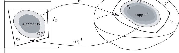
Figure 1: Sketch of the geometric layout of a single chart and its associated cut-off function.

The algorithm under consideration is a Nyström method which produces point-wise values of the unknown $(\psi^{j})$ at the discretization points $\underline{x}_{\underline{m}}^{j}$. The quadrature rules that ultimately define the method are described in what follows; for notational simplicity our approximate quadrature formulae use the set

$$\mathbb{Z}_{N_{j}}:=\big{\{}\underline{m}:=(m_{1},m_{2})\in\mathbb{Z}^{2}:0\leq m_{1},m_{2}\leq N_{j}-1\big{\}}$$ (2.17)

of two-dimensional summation indices $\underline{m}$.

The approximate integration method used by the algorithm to treat the regular portion of the kernel is, simply, based on the trapezoidal rule,

$$\int_{I_{2}}K^{ij}_{{\rm reg},\delta}(\,\cdot\,,\underline{v})\xi(\underline{v}){\rm d}\underline{v}\approx h_{j}^{2}\sum_{\underline{m}\in\mathbb{Z}_{N_{j}}}\!K^{ij}_{{\rm reg},\delta}(\,\cdot\,,\underline{x}^{j}_{\underline{m}})\xi(\underline{x}^{j}_{\underline{m}}),$$ (2.18)

with the convention that $K^{ij}_{{\rm reg},\delta}(\,\cdot\,,\underline{v})\equiv 0$ for $\underline{v}\not\in D^{j}$. Notice that for a $\mathcal{C}^{\infty}$ function $\xi$ compactly supported in

$$\Omega^{j}:=({\bf r}^{j})^{-1}(\mathop{\rm supp}\omega^{j})\subset D^{j},$$ (2.19)

(such as $\xi=(\omega^{j}\psi)\circ{\bf r}^{j}$ with $\psi\in{\cal C}^{\infty}(S)$) the rule embodied in equation (2.18) gives rise to super-algebraic convergence.

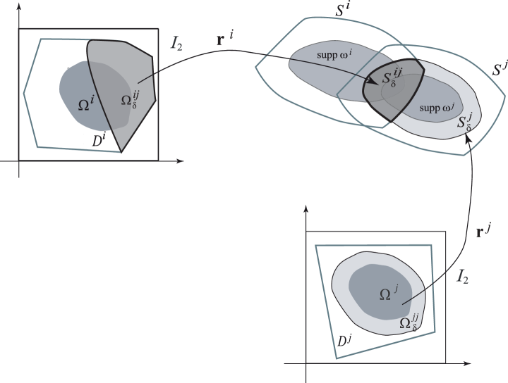
Figure 2: The overlapping of two charts and the associated domains.

To approximate integrals of the form

$$\int_{I_{2}}K^{ij}_{{\rm sing},\delta}(\underline{u},\underline{v})\xi(\underline{v})\mathrm{d}\underline{v},\qquad\xi\in\mathcal{C}^{\infty}(I_{2}),\quad\mathop{\rm supp}\xi\subseteq\Omega^{j},$$ (2.20)

that include the singular part of the kernel, the algorithm uses polar coordinates around the singularity. To properly account for contributions arising from various regions delineated by local charts and overlaps we let

$$\begin{array}[]{c}\underline{r}^{ji}:=({\bf r}^{j})^{-1}\circ{\bf r}^{i}:({\bf r}^{i})^{-1}(S^{i}\cap S^{j})\subset D^{i}\to D^{j}\\[6.45831pt] S^{ij}_{\delta}:=S^{i}\cap S^{j}_{\delta}\subset S^{i}\cap S^{j},\qquad\Omega^{ij}_{\delta}:=({\bf r}^{i})^{-1}(S^{i}\cap S^{j}_{\delta})=({\bf r}^{i})^{-1}(S^{ij}_{\delta});\end{array}$$ (2.21)

see Figure 2 and equation (2.8). A close inspection of the definition of the sets $S^{j}_{\delta}$ shows that $\overline{B({\bf r},\epsilon_{1}\delta)}\cap\mathop{\rm supp}\omega^{j}=\emptyset$ if ${\bf r}\not\in S^{j}_{\delta/2}$. Since, additionally,

$$\mathop{\rm supp}K^{ij}_{{\rm sing},\delta}(\underline{u},\,\cdot\,)\subset\mathop{\rm supp}\eta_{\delta}({\bf r}^{i}(\underline{u}),{\bf r}^{j}(\,\cdot\,))\subset({\bf r}^{j})^{-1}\big{(}\overline{B({\bf r}^{i}(\underline{u}),\epsilon_{1}\delta)}\cap S^{j}\big{)},$$

we conclude that the integral (2.20) with $\mathop{\rm supp}\xi\subseteq\Omega^{j}$, vanishes for all $\underline{u}$ such that ${\bf r}^{i}(\underline{u})\not\in S^{j}_{\delta/2}$, i.e., for $\underline{u}\not\in\Omega_{\delta/2}^{ij}$. The algorithm therefore only produces approximations of (2.20) for $\underline{u}\in\Omega_{\delta/2}^{ij}$. To do this consider the relations

$$\int_{\mathbb{R}^{2}}K^{ij}_{{\rm sing},\delta}(\underline{u},\underline{v})\xi(\underline{v})\mathrm{d}\underline{v}\!$$ (2.22)

$$=\int_{\mathbb{R}^{2}}K_{{\rm sing},\delta}^{ij}\left(\underline{u},\underline{r}^{ji}(\underline{u})+\underline{w}\right)\xi(\underline{r}^{ji}(\underline{u})+\underline{w})\,\mathrm{d}\underline{w}$$

$$=\frac{1}{2}\int_{0}^{2\pi}\bigg{(}\int_{-\infty}^{\infty}|\rho|\,K_{{\rm sing},\delta}^{ij}\left(\underline{u},\underline{r}^{ji}(\underline{u})+\rho\underline{e}(\theta)\right)\,\xi(\underline{r}^{ji}(\underline{u})+\rho\underline{e}(\theta))\,\mathrm{d}\rho\bigg{)}\mathrm{d}\theta$$

where $\underline{e}(\theta):=(\cos\theta,\sin\theta)$ and note that the function

$$(\rho,\theta)\mapsto|\rho|K_{{\rm sing},\delta}^{ij}\left(\underline{u}^{i},\,\underline{r}^{ji}(\underline{u})+\rho\underline{e}(\theta)\right)$$ (2.23)

is smooth (as shown in Section 4, cf. [6, 7]), $2\pi$-periodic in $\theta$ and compactly supported as a function of the variable $\rho$. In what follows we temporarily let $\underline{z}=(z_{1},z_{2}):=\underline{r}^{ji}(\underline{u})$, so that the dependences on the patch indices $(i,j)$ and parametric coordinate $\underline{u}$ are not displayed.

The integral in the angular variable is approximated using a trapezoidal rule on a uniform partition of $[0,2\pi]$ in $\Theta_{j}$ subintervals of length $k_{j}=2\pi/\Theta_{j}$. Therefore, we consider the angles

$$\theta_{p}^{j}:=p\,k_{j},\qquad p=0,\ldots,\Theta_{j}-1$$

and approximate (2.22) by

$$\frac{k_{j}}{2}\sum_{p=0}^{\Theta_{j}-1}\Bigg{(}\int_{-\infty}^{\infty}K^{ij}_{\rm sing,\delta}(\underline{u},\underline{z}+\rho\,\underline{e}(\theta_{p}^{j}))\,|\rho|\,\xi(\underline{z}+\rho\,\underline{e}(\theta_{p}^{j}))\mathrm{d}\rho\Bigg{)}.$$ (2.24)

Recall that a uniform Cartesian grid in $I_{2}$ with mesh length $h_{j}$ has been introduced in the approximation of the regular part (2.18). We will now use points of this grid to approximate the radial integrals in (2.24).

If $|\cos\theta_{p}^{j}|\geq\sqrt{2}/2$, that is, modulo $2\pi$, $\theta_{p}^{j}\in[-\pi/4,\pi/4]\cup[3\pi/4,5\pi/4]$, we look for the intersections

$$\{\underline{x}=\underline{z}+\rho\,e(\theta_{p}^{j})\,:\,\rho\in\mathbb{R}\}\cap\{\underline{x}=(q\,h_{j},\xi)\,:\,\xi\in\mathbb{R}\},\qquad q=0,\ldots,N_{j}-1,$$

i.e., the intersections of the double rays stemming from $\underline{z}$ with angle $\pm\theta_{p}^{j}$ with the vertical lines of the uniform grid: the points of intersections are given by

$$\big{(}q\,h_{j},z_{2}+(q\,h_{j}-z_{1})\tan\theta_{p}^{j}\big{)},\qquad q=0,1,\ldots,N_{j}-1;$$ (2.25)

clearly, the distance between two consecutive points is $h_{j}/|\cos\theta_{p}^{j}|\leq\sqrt{2}h_{j}.$ Alternatively we can express these points in the form

$$\underline{z}+\rho_{q}^{h_{j}}(\underline{z},\theta_{p}^{j})\,\underline{e}(\theta_{p}^{j}),\qquad\mbox{where}\qquad\rho_{q}^{h}(\underline{z},\theta):=\frac{q\,h-z_{1}}{\cos\theta}.$$

For these values of $\theta_{p}^{j}$, the corresponding integral in (2.24) is approximated by

$$h_{j}\,c(\theta_{p}^{j})\sum_{q=0}^{N_{j}-1}K^{ij}_{\rm sing,\delta}\big{(}\underline{u},\underline{z}+\rho_{q}^{h_{j}}(\underline{z},\theta_{p}^{j})\,\underline{e}(\theta_{p}^{j})\big{)}\,|\rho_{q}^{h_{j}}(\underline{z},\theta_{p}^{j})|\,\xi\left(\underline{z}+\rho_{q}^{h_{j}}(\underline{z},\theta_{p}^{j})\,\underline{e}(\theta_{p}^{j})\right),$$ (2.26)

where $c(\theta)=1/|\cos\theta|$. For the remaining angles, intersections are computed with the corresponding horizontal lines:

$$\{\underline{x}=\underline{z}+\rho\,\underline{e}(\theta_{p}^{j})\,:\,\rho\in\mathbb{R}\}\cap\{\underline{x}=(\xi,q\,h_{j})\,:\,\xi\in\mathbb{R}\},\qquad q=0,\ldots,N_{j}-1.$$ (2.27)

The quadrature points are deliberately selected to lie on lines with one of the coordinates equal to $q\,h_{j}$. As discussed in the introduction, such a selection was introduced in [6] to enable fast interpolation of the function $\xi$ on the radial quadrature points (that is, to produce a fast algorithm for evaluation of the operator $R_{N_{j}}$ in (2.33)).

Using the angle-dependent weight

$$c(\theta):=\min\Big{\{}\frac{1}{|\cos\theta|},\frac{1}{|\sin\theta|}\Big{\}},$$ (2.28)

as well as the nodal points radii

$$\rho^{h}_{q}(\underline{z},\theta):=\left\{\begin{array}[]{ll}\displaystyle\frac{qh-z_{1}}{|\cos\theta|},&\mbox{if $|\cos\theta|\geq\sqrt{2}/2$},\\[6.45831pt] \displaystyle\frac{qh-z_{2}}{|\sin\theta|},&\mbox{otherwise},\end{array}\right.$$

expression (2.26) provides approximation of all the integrals in (2.24).

In sum, we define our discrete singular operator (which depends on $h_{j}$ and $k_{j}$, or, equivalently, on $N_{j}$ and $\Theta_{j}$) by

$$(\mathrm{L}^{ij}_{\delta,h}\xi)(\underline{u}):=\left\{\begin{array}[]{l}\displaystyle\frac{h_{j}k_{j}}{2}\!\!\sum_{p=0}^{\Theta_{j}-1}\sum_{q=0}^{N_{j}-1}\!\!c(\theta_{p}^{j})\bigg{(}K^{ij}_{\rm sing,\delta}\Big{(}\underline{u},\underline{r}^{ji}(\underline{u})+\rho_{q}^{h_{j}}(\underline{r}^{ji}(\underline{u}),\theta_{p}^{j})\,\underline{e}(\theta_{p}^{j})\Big{)}\\[6.45831pt] \displaystyle\hskip 39.83368pt\times|\rho_{q}^{h_{j}}(\underline{r}^{ji}(\underline{u}),\theta_{p}^{j})|\,\xi\Big{(}\underline{r}^{ji}(\underline{u})+\rho_{q}^{h_{j}}(\underline{r}^{ji}(\underline{u}),\theta_{p}^{j})\,\underline{e}(\theta_{p}^{j})\Big{)}\bigg{)},\\[6.45831pt] \displaystyle\hfill\mbox{if $\underline{u}\in\Omega^{ij}_{\delta/2}$},\\[6.45831pt] \displaystyle 0,\hfill\mbox{otherwise},\end{array}\right.$$ (2.29)

where $\Omega^{ij}_{\delta/2}=({\bf r}^{i})^{-1}(S^{ij}_{\delta/2})=({\bf r}^{i})^{-1}(S^{i}\cap S^{j}_{\delta/2}).$

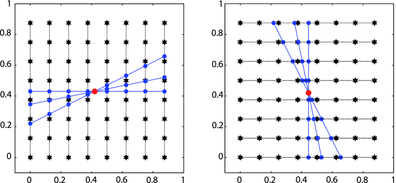
Figure 3: Points used in the integration of the singular part.

In what follows we use the scaling

$$\Theta_{j}\approx N_{j}^{1+\alpha},\qquad\alpha>0,$$ (2.30)

i.e., we assume that there exist $C,c>0$ such that for all $j$, $cN_{j}^{1+\alpha}\leq\Theta_{j}\leq CN_{j}^{1+\alpha}$. We point out that $\rho_{q}^{h}(\underline{z},\,\cdot\,)$ is discontinuous at $\{\pi/4,3\pi/4,5\pi/4,7\pi/4\}$ but both side limits exist. It is immaterial which value (the right or left limit or even the average of both) is set as value to $\rho_{q}^{h}(\underline{z},\,\cdot\,)$ at these points.

2.4 The numerical method

We are now in a position to lay down a fully discrete version of equations (2.15). The unknowns are taken to be approximate values

$$\varphi^{j}_{\underline{\ell}},\qquad\underline{\ell}\in\Omega^{j}_{h}:=\big{\{}\underline{m}\in\mathbb{Z}_{N_{j}}\>:\>{\bf r}^{j}(\underline{x}^{j}_{\underline{m}})\in\mathrm{int}(\mathrm{supp}\,\omega^{j})\big{\}},\qquad j=1,\ldots,J$$ (2.31)

of the true function values $\psi^{j}(\underline{x}^{j}_{\underline{\ell}})$. In what follows we denote by $\bm{\varphi}^{j}\in\mathbb{C}(\Omega^{j}_{h})$ the array whose $\underline{\ell}=(\ell_{1},\ell_{2})$ entry is $\varphi^{j}_{\underline{\ell}}$ for all indices $\underline{\ell}\in\Omega^{j}_{h}$. We consider the set of indices

$$\mathbb{Z}_{N_{j}}^{*}:=\big{\{}\underline{m}:=(m_{1},m_{2})\in\mathbb{Z}^{2}\,:\,-N_{j}/2\leq m_{1},m_{2}<N_{j}/2\big{\}},$$ (2.32)

(note that the cardinality of $\displaystyle\mathbb{Z}_{N_{j}}^{*}$ is $\#\displaystyle\mathbb{Z}^{*}_{N_{j}}=\#\mathbb{Z}_{N_{j}}=N_{j}^{2}$), the space of trigonometric polynomials

$$\mathbb{T}_{N_{j}}:=\mathrm{span}\,\,\big{\{}\exp(2\pi{\rm i}\,\underline{m}\cdot\underline{u})\,\,:\,\,\underline{m}\in\mathbb{Z}_{N_{j}}^{*}\big{\}},$$

the interpolation operator $\mathrm{R}_{N_{j}}:\mathbb{C}(\Omega^{j}_{h})\to\mathbb{T}_{N_{j}}$ defined by the equations

$$\mathrm{R}_{N_{j}}\bm{\varphi}(\underline{x}^{j}_{\underline{\ell}})=\left\{\begin{array}[]{ll}\varphi^{j}_{\underline{\ell}},&\underline{\ell}\in\Omega^{j}_{h},\\[6.45831pt] 0,&\underline{\ell}\in\mathbb{Z}_{N_{j}}\setminus\Omega^{j}_{h},\end{array}\right.$$

and the vectors $\bm{\omega}^{j}\in\mathbb{C}(\Omega^{j}_{h})$ with components $\omega^{j}_{\underline{\ell}}:=\omega^{j}(\mathbf{r}^{j}(\underline{x}^{j}_{\underline{\ell}}))$. Using these notations, the discrete Nyström equations for the system (2.15) are given by

$${\textstyle\frac{1}{2}}\varphi^{i}_{\underline{\ell}}+\sum_{j=1}^{J}h_{j}^{2}\sum_{\underline{m}\in\Omega^{j}_{h}}K^{ij}_{\rm reg,\delta}(\underline{x}^{i}_{\underline{\ell}},\underline{x}^{j}_{\underline{m}})\omega^{j}_{\underline{m}}\,\varphi^{j}_{\underline{m}}+\sum_{j=1}^{J}\Big{(}\mathrm{L}^{ij}_{\delta,h}\mathrm{R}_{N_{j}}(\bm{\omega}^{j}\odot\bm{\varphi}^{j})\Big{)}(\underline{x}_{\underline{\ell}}^{i})$$ (2.33)

$$=-U^{\rm inc}({\bf r}^{i}(\underline{x}^{i}_{\underline{\ell}}))$$

for $\underline{\ell}\in\mathbb{C}(\Omega^{j}_{h})$ and $j=1,\ldots,N$, where the binary operator $\odot$ denotes componentwise product of arrays: for example, $\bm{\omega}^{j}\odot\bm{\varphi}^{j}$ is the array whose $\underline{\ell}$-th entry is given by $\omega^{j}_{\underline{\ell}}\varphi^{j}_{\underline{\ell}}$. Once these point values $\varphi^{j}_{\underline{\ell}}$ have been computed, the Nyström method provides the reconstruction formula

$$\psi^{i}_{h}=-2\sum_{j=1}^{J}\bigg{(}h_{j}^{2}\sum_{\underline{m}\in\Omega^{j}_{h}}K^{ij}_{\rm reg,\delta}(\,\cdot\,,\underline{x}^{j}_{\underline{m}})\omega^{j}_{\underline{m}}\,\varphi^{j}_{\underline{m}}+\mathrm{L}^{ij}_{\delta,h}\mathrm{R}_{N_{j}}(\bm{\omega}^{j}\odot\bm{\varphi}^{j})\bigg{)}-2U^{\rm inc}\circ{\bf r}^{i},$$ (2.34)

($i=1,\ldots,J$). With these definitions, we clearly have

$$\psi^{j}_{h}(\underline{x}^{j}_{\underline{\ell}})=\varphi^{j}_{\underline{\ell}}\qquad\underline{\ell}\in\Omega^{j}_{h}.$$

Finally, the $J$ parameter-space continuous functions $\psi^{j}_{h}:I_{2}\to\mathbb{C}$ can be assembled into a single continuous approximate solution $\psi_{h}({\bf r})$ defined on $S$:

$$\psi_{h}({\bf r}):=\sum_{j\in\mathcal{I}({\bf r})}\omega^{j}({\bf r})\psi^{j}_{h}(({\bf r}^{j})^{-1}({\bf r})),\qquad\mbox{where $\mathcal{I}({\bf r}):=\{j\,:\,{\bf r}\in\mathop{\rm supp}\omega^{j}\}$.}$$ (2.35)

The main convergence result of this paper can now be stated; its proof is given in Sections 3 through 5. The regularity estimates given in the statement of the theorem are expressed in terms of standard Sobolev norms on the surface $S$ (see for instance [1, 21, 23] or any standard text on Sobolev spaces) .

Remark 2.3

The notation $\delta\approx h^{\beta}$ means that

$$ch^{\beta}\leq\delta\leq Ch^{\beta},$$

for some constants $c>0$ and $C>0$, independent of $h$ and $\beta$. Hereafter, the parameter $\beta\in(0,1)$ will be taken to be fixed. Dependence of constants on this parameter will not be shown explicitly.

Theorem 2.1

Let $\psi$ be the solution of (2.2), and assume $\delta\approx h^{\beta}$ with $\beta\in(0,1)$. Then for sufficiently large values of $N$ the Nyström equations (2.33) admit a unique solution. Letting $\psi_{h}$ denote the reconstructed function on $S$ as defined by (2.34) and (2.35), we have the error estimate

$$\|\psi_{h}-\psi\|_{L^{2}(S)}\leq C_{t}\big{(}|\log h|^{\frac{3}{2}}h^{t(1-\beta)}+h^{t-1}\big{)}\|\psi\|_{H^{t}(S)},$$ (2.36)

for all $t\geq 2$. Finally, for all $\varepsilon>0$ and $t\geq 2$

$$\|\psi_{h}-\psi\|_{L^{\infty}(S)}\leq C_{t,\varepsilon}\big{(}h^{t(1-\beta)-(1+\varepsilon)\beta}+h^{t-1}\big{)}\|\psi\|_{H^{t}(S)}.$$ (2.37)

Theorem 2.1 tells us that for a smooth surface $S$ and a $\mathcal{C}^{\infty}$ right-hand side $U^{\mathrm{inc}}$ (from which it follows that $\psi\in\mathcal{C}^{\infty}(S)$) the Nyström algorithm under consideration converges super-algebraically fast.

Remark 2.4

As mentioned in Section 2.2, the parameter $\delta\approx h^{\beta}$ plays central roles in both the theory and the actual performance of the the algorithm under consideration. With regards to the latter we briefly mention here that use of the floating cut-off function (2.10), whose support is controlled by the parameter $\delta$, helps restrict the use of the costly polar integration scheme to a small region around the singular point (thus reducing the overall computing time required by the algorithm), and, further, it enables acceleration via a sparse, parallel-face FFT-based equivalent-source technique; see [6] for details. (In particular we note that the value $\beta=1/3$ is used in [6, 7] for optimal speed of the equivalent-source accelerated Nyström method.) The parameter $\delta\approx h^{\beta}$ also has a significant impact on our theoretical treatment. Indeed, one of the most delicate points in our stability analysis concerns the convergence in norm of a discrete singular operator to a corresponding continuous singular operator. One of the terms in our estimate of the norm of the difference of these operators (equation (5.18) in Proposition 5.7) is bounded by $|\log h|^{3/2}h^{\beta/2}$. By taking $\beta>0$ we ensure that this terms also tends to zero, from which the desired convergence in norm results.

3 Biperiodic framework

3.1 Continuous equations

The analysis of the method will be carried out by recasting the system (2.15) as a system of periodic integral equations with all unknown functions defined on the unit square $I_{2}$. To introduce our periodic formulation we utilize a second family of cut-off functions, $\widetilde{\omega}^{j}_{\delta}\in{\cal C}^{\infty}(I_{2})$, that depends on $\delta$ and satisfies the following assumptions:

$$\mathop{\rm supp}\widetilde{\omega}^{j}_{\delta}\subset\Omega^{jj}_{3\delta/2}=({\bf r}^{j})^{-1}(S^{j}_{3\delta/2}),$$ (3.1a)

$$\widetilde{\omega}_{\delta}^{j}\ \equiv\ 1\quad\mbox{ in }\Omega^{jj}_{\delta}=({\bf r}^{j})^{-1}(S^{j}_{\delta})\supset\Omega^{j},$$ (3.1b)

$$\|\partial_{\underline{\alpha}}\widetilde{\omega}_{\delta}^{j}\|_{\infty,I_{2}}\leq C_{\underline{\alpha}}\delta^{-|\underline{\alpha}|}\qquad\forall\underline{\alpha}\geq\underline{0},$$ (3.1c)

where for a given non-negative bi-index $\underline{\alpha}=(\alpha_{1},\alpha_{2})$,

$$\partial_{\underline{\alpha}}\xi(\underline{u})=\partial^{\alpha_{1}}_{{u}_{1}}\partial^{\alpha_{2}}_{{u}_{2}}\xi(u_{1},u_{2})$$

and $\|\cdot\|_{\infty,I_{2}}$ is the $L^{\infty}(I_{2})$ norm. We will use the characteristic function

$$\widetilde{\omega}_{0}^{j}(\underline{u}):=\left\{\begin{array}[]{ll}1&\mbox{if }\underline{u}\in\Omega^{j},\\ 0&\mbox{otherwise},\\ \end{array}\right.$$ (3.2)

which can be viewed as the limit of $\widetilde{\omega}^{j}_{\delta}$ as $\delta\to 0$.

Using these functions, we define the following periodic integral operators

$$\mathrm{A}^{ij}_{\rm reg,\delta}\xi := (\omega^{i}\circ{\bf r}^{i})\int_{I_{2}}K^{ij}_{\rm reg,\delta}(\,\cdot\,,\underline{u})\widetilde{\omega}^{j}_{\delta}(\underline{u})\xi(\underline{u}){\rm d}\underline{u},$$ (3.3)

$$\mathrm{A}^{ij}_{\rm sing,\delta}\xi := (\omega^{i}\circ{\bf r}^{i})\int_{I_{2}}K^{ij}_{\rm sing,\delta}(\,\cdot\,,\underline{u})\widetilde{\omega}^{j}_{\delta}(\underline{u})\xi(\underline{u}){\rm d}\underline{u},$$ (3.4)

$$\mathrm{A}^{ij}_{\delta}\xi := (\mathrm{A}^{ij}_{\rm reg,\delta}+\mathrm{A}^{ij}_{\rm sing,\delta})\xi,$$ (3.5)

as well as the right-hand sides $U^{i}:=-(\omega^{i}U^{\rm inc})\circ{\bf r}^{i}$, properly extended by zero to the full unit square $I_{2}$. If $\underline{u}\in I_{2}\setminus\Omega^{ij}_{2\delta}$, then ${\bf r}^{i}(\underline{u})\not\in S^{j}_{2\delta}$ and

$$\mathop{\rm supp}(K^{ij}_{\mathrm{sing},\delta}(\underline{u},\,\cdot\,)\,\widetilde{\omega}^{j}_{\delta}) \subset \mathop{\rm supp}\eta_{\delta}({\bf r}^{i}(\underline{u}),{\bf r}^{j}(\,\cdot\,))\cap\mathop{\rm supp}\widetilde{\omega}^{j}_{\delta}$$

$$\subset \mathop{\rm supp}\eta_{\delta}({\bf r}^{i}(\underline{u}),{\bf r}^{j}(\,\cdot\,))\cap\Omega^{jj}_{3\delta/2}=\emptyset$$

by (2.12) and (3.1a), which implies that

$$(\mathrm{A}^{ij}_{\rm sing,\delta}\xi)(\underline{u})=0\qquad\forall\underline{u}\in I_{2}\setminus\Omega^{ij}_{2\delta}.$$ (3.6)

Letting $\psi^{j}:=\psi\circ{\bf r}^{j}$ be as in equation (2.15) and since $\widetilde{\omega}_{\delta}^{j}\>(\omega^{j}\circ{\bf r}^{j})\equiv\omega^{j}\circ{\bf r}^{j}$ (see (3.1b) and note that $\mathop{\rm supp}(\omega^{j}\circ{\bf r}^{j})\subset\Omega^{jj}_{\delta}$), we see that the functions

$$\phi^{j}:=(\omega^{j}\psi)\circ{\bf r}^{j}=(\omega^{j}\circ{\bf r}^{j})\psi^{j}:I_{2}\to\mathbb{C}\qquad j=1,\ldots,J$$ (3.7)

extended by zero outside $\Omega^{j}=\mathop{\rm supp}(\omega^{j}\circ{\bf r}^{j})$ constitute a solution of the system

$${\textstyle\frac{1}{2}}\phi^{i}+\sum_{j=1}^{J}\mathrm{A}^{ij}_{\rm reg,\delta}\phi^{j}+\sum_{j=1}^{J}\mathrm{A}^{ij}_{\rm sing,\delta}\phi^{j}=U^{i},\qquad i=1,\ldots,J.$$ (3.8)

Equation (3.8) amounts to a system of equations for the vector $(\phi^{j})\in\left(L^{2}(I_{2})\right)^{J}$ for a given right-hand side $(V^{i})\in\left(L^{2}(I_{2})\right)^{J}$. With this understanding, Theorem 3.2 shows that the system (3.8) has a unique solution for any right-hand side $(U^{i})\in\left(L^{2}(I_{2})\right)^{J}$. (It follows that for the particular right-hand side (3.8) the solution is (3.7)—which, clearly, is independent of $\delta$ in spite of the $\delta$-dependence of the system of equations (3.8).) Theorem 3.1 shows that for the case $U^{i}:=-(\omega^{i}U^{\rm inc})\circ{\bf r}^{i}$, the solution of (2.2) can be reconstructed from the solution of (3.8).

3.2 Analysis of the continuous system

Theorem 3.1

Let $(\phi^{1},\ldots,\phi^{J})$ be a solution of (3.8) with $U^{i}:=-(\omega^{i}U^{\mathrm{inc}})\circ{\bf r}^{i}$. Then the solution of (2.2) can be expressed in the form

$$\psi({\bf r}):=\sum_{j\in\mathcal{I}({\bf r})}\phi^{j}(({\bf r}^{j})^{-1}({\bf r})),$$

see equation (2.35).

Proof. Because of the particular form of the right-hand side as well as the presence of the factor $\omega^{i}\circ{\bf r}^{i}$ in the operator $\mathrm{A}^{ij}_{\delta}$ (see equations (3.3), (3.4) and  (3.8)), it follows that $\mathop{\rm supp}\phi^{i}\subseteq\mathop{\rm supp}(\omega^{i}\circ{\bf r}^{i})=\Omega^{i}$. Therefore, by (3.1b), $\widetilde{\omega}^{i}_{\delta}\phi^{i}\equiv\phi^{i}$ for all $i$.

Consider now the functions $\psi^{i}:D^{i}\to\mathbb{C}$ given by

$$\psi^{i}:=-2\sum_{j=1}^{J}\int_{I_{2}}K^{ij}(\,\cdot\,,\underline{v})\phi^{j}(\underline{v})\mathrm{d}\underline{v}-2\,U^{\mathrm{inc}}\circ{\bf r}^{i}.$$

These functions are constructed so that $\phi^{i}=(\omega^{i}\circ{\bf r}^{i})\,\psi^{i}$ for all $i$. Although the functions $\psi^{i}$ are infinitely differentiable only up to the boundary of $D^{i}$ (the domain of the chart ${\bf r}^{i}$), the function $\phi^{i}$ can be smoothly extended by zero to $\mathbb{R}^{2}$. Similarly, we can consider the functions $\Phi^{i}:S\to\mathbb{C}$ such that $\Phi^{i}({\bf r})=\omega^{i}({\bf r})\psi^{i}(({\bf r}^{i})^{-1}({\bf r}))=\phi^{i}(({\bf r}^{i})^{-1}({\bf r}))$ if ${\bf r}\in S^{i}$ and are zero otherwise. These are $\mathcal{C}^{\infty}$ functions on the surface $S$ and $\psi=\sum_{j=1}^{J}\Phi^{j}$.

Then, if ${\bf r}\in S$ and $i\in\mathcal{I}({\bf r})$, we can write ${\bf r}={\bf r}^{i}(\underline{u}^{i})$ with $\underline{u}^{i}:=({\bf r}^{i})^{-1}({\bf r})$, and

$$({\textstyle\frac{1}{2}}\psi+A\psi)({\bf r}) = {\textstyle\frac{1}{2}}\sum_{i\in\mathcal{I}({\bf r})}\phi^{i}(\underline{u}^{i})+\sum_{i=1}^{J}\omega^{i}({\bf r})(A\psi)({\bf r})$$

$$= \sum_{i\in\mathcal{I}({\bf r})}\Big{(}{\textstyle\frac{1}{2}}\phi^{i}(\underline{u}^{i})+\omega^{i}({\bf r})\int_{S}K({\bf r},{\bf r}^{\prime})\Big{(}\sum_{j=1}^{J}\Phi^{j}({\bf r}^{\prime})\Big{)}\mathrm{d}\mathbf{r}^{\prime}\Big{)}$$

$$= \sum_{i\in\mathcal{I}({\bf r})}\Big{(}{\textstyle\frac{1}{2}}\phi^{i}(\underline{u}^{i})+\sum_{j=1}^{J}\omega^{i}({\bf r})\int_{\mathop{\rm supp}\omega^{j}}K({\bf r},{\bf r}^{\prime})\Phi^{j}({\bf r}^{\prime})\mathrm{d}{\bf r}^{\prime}\Big{)}$$

$$= \sum_{i\in\mathcal{I}({\bf r})}\Big{(}{\textstyle\frac{1}{2}}\phi^{i}(\underline{u}^{i})+\sum_{j=1}^{J}\omega^{i}({\bf r})\int_{I_{2}}K({\bf r},{\bf r}^{j}(\underline{v}))\,a^{j}(\underline{v})\,\phi^{j}(\underline{v})\,\mathrm{d}\underline{v}\Big{)}$$

$$= \sum_{i\in\mathcal{I}({\bf r})}\Big{(}{\textstyle\frac{1}{2}}\phi^{i}(\underline{u}^{i})+\sum_{j=1}^{J}\omega^{i}({\bf r}^{i}(\underline{u}^{i}))\int_{I_{2}}K^{ij}(\underline{u}^{i},\underline{v})\widetilde{\omega}^{j}_{\delta}(\underline{v})\phi^{j}(\underline{v})\mathrm{d}\underline{v}\Big{)}$$

$$= \sum_{i\in\mathcal{I}({\bf r})}\Big{(}{\textstyle\frac{1}{2}}\phi^{i}(\underline{u}^{i})+\sum_{j=1}^{J}\mathrm{A}^{ij}_{\delta}\phi^{j}(\underline{u}^{i})\Big{)}=\sum_{i\in\mathcal{I}({\bf r})}U^{i}(\underline{u}^{i})=-U^{\mathrm{inc}}({\bf r}).$$

Note that we have used the fact that $\widetilde{\omega}^{j}_{\delta}\phi^{j}\equiv\phi^{j}$. This finishes the proof. $\Box$

The product space

$${\cal H}^{s}:=\underbrace{{H}^{s}\times{H}^{s}\times\cdots\times{H}^{s}}_{\mbox{$J$ times}},$$

will be endowed with the product norm, also denoted by $\|\cdot\|_{s}$. We can then consider the matrices of operators

$${\mathcal{A}}^{\rm reg}_{\delta}:=\left(\mathrm{A}^{ij}_{\rm reg,\delta}\right)_{i,j=1}^{J},\quad{\mathcal{A}}^{\rm sing}_{\delta}:=\left(\mathrm{A}^{ij}_{\rm sing,\delta}\right)_{i,j=1}^{J},\qquad{\mathcal{A}}_{\delta}:={\mathcal{A}}^{\rm reg}_{\delta}+{\mathcal{A}}_{\delta}^{\rm sing},$$

as well as the identity operator ${\cal I}:{\cal H}^{s}\to{\cal H}^{s}$. With this notation, (3.8) can be written in operator form as

$${\mathcal{B}}_{\delta}\bm{\phi}:=({\textstyle\frac{1}{2}}{\cal I}+{\mathcal{A}}_{\delta})\bm{\phi}={\bf U}$$ (3.9)

where $\bm{\phi}:=(\phi^{1},\phi^{2},\ldots,\phi^{J})$ and

$$\mathbf{U}:=\left(U^{1},\ldots,U^{J}\right)\qquad U^{j}=-(\omega^{j}U^{\mathrm{inc}})\circ{\bf r}^{j}.$$ (3.10)

Remark 3.1

Note that, while the operator ${\mathcal{A}}_{\delta}$ depends on $\delta$, equations (3.3)-(3.5) show that, for elements $\bm{\phi}=(\phi^{1},\ldots,\phi^{J})$ such that $\mathrm{supp}\,\phi^{i}\subseteq\mathop{\rm supp}(\omega^{i}\circ{\bf r}^{i})$, $\mathcal{A}_{\delta}\bm{\phi}$ is independent of $\delta$. The following theorem shows that the operator in equation (3.9) is invertible, and, thus, in view of Theorem 3.1, for right-hand sides of the form (3.10), the solution of equation (3.9) is independent of $\delta$ as well.

Theorem 3.2

For all  $0\leq\delta\leq\delta_{0}$, the operators $\mathcal{B}_{\delta}=\frac{1}{2}\mathcal{I}+\mathcal{A}_{\delta}:\mathcal{H}^{0}\to\mathcal{H}^{0}$ are invertible. Moreover

$$\|\mathcal{B}_{\delta}\|_{\mathcal{H}^{0}\to\mathcal{H}^{0}}+\|\mathcal{B}_{\delta}^{-1}\|_{\mathcal{H}^{0}\to\mathcal{H}^{0}}\leq C.$$

Proof. We will first show that ${\mathcal{B}}_{\delta}:{\cal H}^{0}\to{\cal H}^{0}$ is invertible. Propositions 3.4 and 3.6 and the compact injection $H^{1}\subset H^{0}$ prove that ${\mathcal{A}}_{\delta}:{\cal H}^{0}\to{\cal H}^{0}$ is compact (and uniformly bounded in $\delta$). Therefore, ${\mathcal{B}}_{\delta}:{\cal H}^{0}\to{\cal H}^{0}$ is bounded and Fredholm of index zero. Thus, it suffices to prove the injectivity of the operator.

Let then $\bm{\phi}\in{\rm Ker}\,{\mathcal{B}}_{\delta}$, that is,

$${\textstyle\frac{1}{2}}\phi^{i}+\sum_{j=1}^{J}\mathrm{A}^{ij}_{\delta}\phi^{j}=0,\qquad i=1,\ldots,J.$$

Arguing as in the proof of Theorem 3.1, it is clear that $\widetilde{\omega}_{\delta}^{j}\phi^{j}\equiv\phi^{j}$ for all $j$, which means that $\mathrm{Ker}\,\mathcal{B}_{\delta}$ is independent of $\delta$. Since $\mathrm{A}^{ij}_{\delta}:H^{s}\to H^{s+1}$ are continuous for all $s$, then $\phi^{i}\in{\cal C}^{\infty}(\overline{I}_{2})$. Following the argumentation in the proof of Theorem 3.1, we define

$$\psi^{i}:=-2\sum_{j=1}^{J}\int_{I_{2}}K^{ij}(\,\cdot\,,\underline{v})\widetilde{\omega}_{\delta}^{j}(\underline{v})\phi^{j}(\underline{v})\,{\rm d}\underline{v}=-2\sum_{j=1}^{J}\int_{I_{2}}K^{ij}(\,\cdot\,,\underline{v})\phi^{j}(\underline{v})\mathrm{d}\underline{v},$$ (3.11)

so that $\phi^{i}=(\omega^{i}\circ{\bf r}^{i})\psi^{i}$. We now set

$$\psi({\bf r}):=\sum_{j\in\mathcal{I}({\bf r})}\phi^{j}(({\bf r}^{j})^{-1}({\bf r}))=\sum_{j=1}^{J}\Phi^{j}({\bf r}),$$

where the functions $\Phi^{j}:S\to\mathbb{C}$ are defined by extending $\omega^{j}\,\psi^{j}\circ({\bf r}^{j})^{-1}=\phi^{j}\circ({\bf r}^{j})^{-1}$ by zero to $S\setminus S^{j}$. Proceeding as before, we prove that $\frac{1}{2}\psi+A\psi=0$ and therefore $\psi=0$.

From (3.11) we deduce that for $\underline{u}\in D^{i}$,

$$\psi^{i}(\underline{u}) = -2\sum_{j=1}^{J}\int_{I_{2}}K^{ij}(\underline{u},\underline{v})\,\phi^{j}(\underline{v})\,{\rm d}\underline{v}=-2\sum_{j=1}^{J}\int_{S^{j}}K({\bf r}^{i}(\underline{u}),{\bf r}^{\prime})\Phi^{j}({\bf r}^{\prime})\,\mathrm{d}{\bf r}^{\prime}$$

$$= -2\int_{S}K({\bf r}^{i}(\underline{u}),{\bf r}^{\prime})\psi({\bf r}^{\prime})\,{\rm d}{\bf r}^{\prime}=0$$

since $\psi$ itself is zero and the functions $\Phi^{j}$ are each supported in $S^{j}$. Therefore $\phi^{i}=(\omega^{i}\circ{\bf r}^{i})\psi^{i}=0$ and the injectivity of $\mathcal{B}_{\delta}$ is proven.

To prove the uniform boundedness of ${\mathcal{B}}_{\delta}^{-1}:{\cal H}^{0}\to{\cal H}^{0}$ for $\delta\geq 0$ we proceed as in the proof of Theorem 10.9 in [19]. Recall that ${\mathcal{A}}_{\delta}:{\cal H}^{0}\to{\cal H}^{1}$ is uniformly bounded in $\delta$ by Proposition 3.4 with $s=0$. Since the injection ${\cal H}^{1}\subset{\cal H}^{0}$ is compact, the set $\{{\mathcal{A}}_{\delta}\}_{\delta}$ turns out to be collectively compact. Moreover, it is easy to verify that $\lim_{\delta\to 0}{\mathcal{A}}_{\delta}\bm{\xi}=\mathcal{A}_{0}\bm{\xi}$ in $\mathcal{H}^{0}$ for all $\bm{\xi}\in\mathcal{H}^{0}$. Applying that pointwise convergence is uniform on compact sets and the collective compactness of the set of operators $\{\mathcal{A}_{\delta}\}$ it follows (see [19, Corollaries 10.5 and 10.8]) that

$$\|{\mathcal{B}}_{0}^{-1}({\mathcal{A}}_{0}-{\mathcal{A}}_{\delta}){\mathcal{A}}_{\delta}\|_{{\cal H}^{0}\to{\cal H}^{0}}\to 0.$$ (3.12)

Consider now ${\cal C}_{\delta}:=2(\mathcal{I}-{\mathcal{B}}_{0}^{-1}{\mathcal{A}}_{\delta})$, which is uniformly bounded. Straightforward computations show that

$${\cal C}_{\delta}{\mathcal{B}}_{\delta}={\cal I}+2{\mathcal{B}}_{0}^{-1}({\mathcal{B}}_{0}{\mathcal{A}}_{\delta}-{\mathcal{B}}_{\delta}{\mathcal{A}}_{\delta})={\cal I}+2{\mathcal{B}}_{0}^{-1}({\mathcal{A}}_{0}-{\mathcal{A}}_{\delta}){\mathcal{A}}_{\delta}.$$

Therefore (3.12) proves that for $\delta$ small enough $\mathcal{C}_{\delta}\mathcal{B}_{\delta}$ is invertible with uniformly bounded inverse and therefore, since $\mathcal{C}_{\delta}$ is uniformly bounded, so is $\mathcal{B}_{\delta}^{-1}.$ $\Box$

3.3 Discrete system

In order to obtain a continuous system of equations from the fully discrete system (2.33) we introduce an interpolation operator $\mathrm{Q}_{N_{j}}:{\cal C}^{0}(\overline{I}_{2})\to\mathbb{T}_{N_{j}}$ given by

$$(\mathrm{Q}_{N_{j}}\xi)(\underline{x}^{j}_{\underline{\ell}})=\xi(\underline{x}^{j}_{\underline{\ell}})\qquad\forall\underline{\ell}\in\mathbb{Z}_{N_{j}}.$$ (3.13)

The discrete counterparts of the functions $\phi^{j}$ are

$$\phi^{j}_{h}:=\mathrm{Q}_{N_{j}}((\omega^{j}\circ{\bf r}^{j})\psi^{j}_{h}),\\$$ (3.14)

where $\psi^{j}_{h}$ is defined by (2.34) with $\varphi^{j}_{\underline{m}}$ obtained as the solution of the system (2.33). Note that

$$\phi^{j}_{h}(\underline{x}^{j}_{\underline{\ell}})=\mathrm{Q}_{N_{j}}((\omega^{j}\circ{\bf r}^{j})\>\psi^{j}_{h})(\underline{x}_{\underline{\ell}}^{j})=\mathrm{R}_{N_{j}}(\bm{\omega}^{j}\odot\bm{\varphi}^{j})(\underline{x}_{\underline{\ell}}^{j})=\left\{\begin{array}[]{ll}\omega^{j}_{\underline{\ell}}\,\varphi^{j}_{\underline{\ell}},&\mbox{if }\underline{\ell}\in\Omega^{j}_{h},\\[4.30554pt] 0,&{\rm otherwise}.\end{array}\right.$$ (3.15)

On the other hand, $\big{(}\widetilde{\omega}^{j}_{\delta}\phi^{j}_{h}\big{)}(\underline{x}_{\underline{\ell}}^{j})=\phi^{j}_{h}(\underline{x}_{\underline{\ell}}^{j})$ for all $\underline{\ell}$, since $\phi^{j}_{h}(\underline{x}_{\underline{\ell}}^{j})=0,$ for all $\underline{\ell}\not\in\Omega^{j}_{h}$ and inside $\Omega^{j}$ the functions $\widetilde{\omega}^{j}$ do not have any influence by (3.1b). Therefore (2.33) can be equivalently re-expressed as an equation for continuous biperiodic functions $(\phi^{1}_{h},\ldots,\phi^{J}_{h})$ such that for all $i\in\{1,\ldots,J\}$

$${\textstyle\frac{1}{2}}\phi^{i}_{h}+\sum_{j=1}^{J}\mathrm{Q}_{N_{i}}\bigg{(}h_{j}^{2}\sum_{\underline{m}\in\mathbb{Z}_{N_{j}}}\left(\omega^{i}\circ{\bf r}^{i}\right)K^{ij}_{\rm reg,\delta}(\,\cdot\,,\underline{x}_{\underline{m}}^{j})\widetilde{\omega}^{j}_{\delta}(\underline{x}^{j}_{\underline{m}})\phi_{h}^{j}(\underline{x}_{\underline{m}}^{j})\bigg{)}$$

$$+\sum_{j=1}^{J}\mathrm{Q}_{N_{i}}\Big{(}(\omega^{i}\circ{\bf r}^{i})\mathrm{L}^{ij}_{\delta,h}\phi^{j}_{h}\Big{)} = \mathrm{Q}_{N_{i}}U^{i}.\qquad\ \$$ (3.16)

Note that if the system (3.16) is uniquely solvable, the solution belongs necessarily to $\mathbb{T}_{N_{1}}\times\cdots\times\mathbb{T}_{N_{J}}$. The solutions of (2.33) and (3.16) are related by the formula (3.15).

For the sake of our analysis we recast the system (3.16) in an equivalent operator form. To do this, we introduce the discrete operators

$$\mathrm{A}^{ij}_{{\rm sing},\delta,h}:=(\omega^{i}\circ{\bf r}^{i})\mathrm{L}^{ij}_{\delta,h},$$ (3.17)

and, for $\xi\in\mathcal{C}^{0}(\overline{I}_{2})$, we define (cf. [10] and [14])

$$\mathrm{D}_{N_{j}}\xi:=h_{j}^{2}\sum_{\underline{m}\in\mathbb{Z}_{N_{j}}}\xi(\underline{x}^{j}_{\underline{m}})\delta_{\underline{x}_{\underline{m}}^{j}},$$ (3.18)

where $\delta_{\underline{u}}$ denotes here the Dirac delta distribution at the point $\underline{u}\in\overline{I}_{2}$: $\delta_{\underline{u}}\psi:=\psi(\underline{u})$. Further, we note that since the operators $\mathrm{A}^{ij}_{\rm reg,\delta}$ have continuous kernels, they may be applied to delta distributions:

$$\mathrm{A}^{ij}_{\rm reg,\delta}\delta_{\underline{u}}=\left(\omega^{i}\circ{\bf r}^{i}\right)K^{ij}_{\rm reg,\delta}(\hskip 2.0pt\cdot\hskip 2.0pt,{\underline{u}})\widetilde{\omega}^{j}_{\delta}({\underline{u}}).$$

In view of these definitions, we clearly have

$$\mathrm{A}^{ij}_{\rm reg,\delta}\mathrm{D}_{N_{j}}\xi=h_{j}^{2}\sum_{\underline{m}\in\mathbb{Z}_{N_{j}}}\left(\omega^{i}\circ{\bf r}^{i}\right)K^{ij}_{\rm reg,\delta}(\hskip 2.0pt\cdot\hskip 2.0pt,\underline{x}_{\underline{m}}^{j})\widetilde{\omega}^{j}_{\delta}(\underline{x}^{j}_{\underline{m}})\xi(\underline{x}_{\underline{m}}^{j}),$$

and (3.16) is equivalent to the equation

$${\textstyle\frac{1}{2}}\phi^{i}_{h}+\sum_{j=1}^{J}\mathrm{Q}_{N_{i}}\Big{(}\mathrm{A}^{ij}_{\rm reg,\delta}\mathrm{D}_{N_{j}}\phi^{j}_{h}+\mathrm{A}^{ij}_{{\rm sing},\delta,h}\phi^{j}_{h}\Big{)}=\mathrm{Q}_{N_{i}}U^{i},\qquad i=1,\ldots,J,$$ (3.19)

for the unknowns $(\phi^{1}_{h},\ldots,\phi^{J}_{h})\in\mathbb{T}_{N_{1}}\times\cdots\times\mathbb{T}_{N_{J}}$.

In order to recast this system of operator equations as a system defined in $L^{2}$ spaces, we insert the orthogonal projections $\mathrm{P}_{N_{j}}:L^{2}(I_{2})\to\mathbb{T}_{N_{j}}$ and write (3.16) in the form

$${\textstyle\frac{1}{2}}\phi^{i}_{h}+\sum_{j=1}^{J}\mathrm{Q}_{N_{i}}\Big{(}\mathrm{A}^{ij}_{\rm reg,\delta}\mathrm{D}_{N_{j}}\mathrm{P}_{N_{j}}\phi^{j}_{h}+\mathrm{A}^{ij}_{{\rm sing},\delta,h}\mathrm{P}_{N_{j}}\phi^{j}_{h}\Big{)}=\mathrm{Q}_{N_{i}}U^{i},\qquad i=1,\ldots,J.$$ (3.20)

for the unknowns $(\phi^{1}_{h},\ldots,\phi^{J}_{h})\in L^{2}(I_{2})\times\cdots\times L^{2}(I_{2})$.

Remark 3.2

Note that the projection operator $\mathrm{P}_{N_{j}}$, which maps $L^{2}$ to the space of trigonometric polynomials, makes it possible to recast the fully discrete equation (3.16) (whose unknowns are approximate point values of the continuous solution of equation (2.15)) via its version (3.19), posed in the space of trigonometric polynomials, as an equation (3.20) in the complete space $L^{2}$.

3.4 Mapping properties of the operators introduced in Section 3.1

As a result of the work in Sections 3.1 and 3.3, our overall integral equation and its Nyström discretization have been re-expressed as equations (3.8) and (3.20), respectively, which are posed in terms of unknowns defined (and compactly supported) on the open unit square $I_{2}$. Such functions can naturally be extended to period-1 biperiodic functions defined in $\mathbb{R}^{2}$, on which our analysis is based. In this section, in particular, we study the mapping properties of the operators introduced in Section 3.1, when viewed as operators defined on spaces of periodic functions.

To do this we first consider the biperiodic Sobolev spaces, see e.g. [22], and we study their connections (that result through our use of local charts and partitions of unity) with the classical Sobolev spaces on the surface $S$. The Fourier coefficients of any locally integrable biperiodic function $\xi:\mathbb{R}^{2}\to\mathbb{C}$ are given by

$$\widehat{\xi}(\underline{m}):=\int_{I_{2}}\xi(\underline{u})e_{\underline{m}}(\underline{u})\mathrm{d}\underline{u},\qquad e_{\underline{m}}(\underline{u}):=\exp(2\pi{\rm i}\underline{m}\cdot\underline{u}),\quad\underline{m}\in\mathbb{Z}^{2}.$$

For arbitrary $s\in\mathbb{R}$, the Sobolev norm

$$\|\xi\|_{s}:=\Big{(}|\widehat{\xi}(\underline{0})|^{2}+\sum_{\underline{m}\neq\underline{0}}(|m_{1}|^{2}+|m_{2}|^{2})^{s}|\widehat{\xi}(\underline{m})|^{2}\Big{)}^{1/2}$$ (3.21)

is well defined for all $\xi$ in the space $\mathbb{T}:=\mathrm{span}\{e_{\underline{m}}\,:\,\underline{m}\in\mathbb{Z}^{2}\}=\cup_{N}\mathbb{T}_{N}$ of trigonometric polynomials. The Sobolev space $H^{s}$ is defined as the completion of $\mathbb{T}$ under the norm $\|\,\cdot\,\|_{s}$. Note that $H^{0}$ is the space of biperiodic extensions of functions in $L^{2}(I_{2})$. By a simple density argument, we can define the Fourier coefficients for any element of $H^{s}$ and any $s<0$. It is also possible to define partial derivatives of any order: for a given non-negative bi-index $\underline{\alpha}=(\alpha_{1},\alpha_{2})$, using the notation $|\underline{\alpha}|=\alpha_{1}+\alpha_{2}$, we see that $\partial_{\underline{\alpha}}$ is a bounded operator from $H^{s}$ to $H^{s-|\underline{\alpha}|}$ for all $s$.

The atlas introduced in Section 2 for representation of the surface $S$ together with the $H^{s}$ norm just defined gives rise to a definition of the Sobolev norm

$$\|U\|_{H^{s}(S)}:=\bigg{(}\sum_{i=1}^{J}\|(\omega^{i}U)\circ{\bf r}^{i}\|^{2}_{s}\bigg{)}^{1/2}$$ (3.22)

for any $U\in\mathcal{C}^{\infty}(S)$ and any $s\in\mathbb{R}$. (In this formula it has been implicitly assumed that, even though ${\bf r}^{i}$ is only defined on $D^{i}\subset I_{2}$, the function $(\omega^{i}U)\circ{\bf r}^{i}$ can be extended by zero to a function in $\mathcal{C}^{\infty}(I_{2})$—since the support of $\omega^{i}\circ{\bf r}^{i}$ is contained in $D^{i}$—and the result can be extended as a $\mathcal{C}^{\infty}$ biperiodic function to all of $\mathbb{R}^{2}$.) The space $H^{s}(S)$ can then be then defined, for instance, as the completion of ${\cal C}^{\infty}(S)$ in the above norm: this definition is equivalent to the classical definitions given in e.g. [1], [17, §1.3.3], [23, §2.4] and [21, Chapter 3].

Lemma 3.3

For all $s\in\mathbb{R}$ and $j\in\{1,\ldots,J\}$

$$\|(\widetilde{\omega}_{\delta}^{j}\xi)\circ({\bf r}^{j})^{-1}\|_{H^{s}(S)}\leq C_{s}\delta^{-|s|}\|\xi\|_{s}\qquad\forall\xi\in H^{s},\qquad\forall\delta,$$ (3.23)

where $C_{s}$ is a constant independent of $\delta$.

Proof. Because of (3.22) we only need to prove that the maps

$$\xi\longmapsto\mathrm{T}^{ji}_{\delta}\xi:=\underbrace{(\omega^{i}\circ{\bf r}^{i})(\widetilde{\omega}^{j}_{\delta}\circ\underline{r}^{ji})}_{=:\varrho_{\delta}^{ji}}\,(\xi\circ\underline{r}^{ji})$$ (3.24)

map $H^{s}$ to $H^{s}$ for every $s$ and that their norms are bounded by a multiple of $\delta^{-|s|}$. To do this we first note that

$$\mathop{\rm supp}\varrho^{ji}_{\delta}\subset({\bf r}^{i})^{-1}(S^{j}\cap S^{i}),$$ (3.25)

(which is the domain where $\underline{r}^{ji}$ is defined), and that, in view of equation (3.1c), we have

$$\|\partial_{\underline{\alpha}}\varrho^{ji}_{\delta}\|_{\infty,I_{2}}\leq C_{\underline{\alpha}}\delta^{-|\alpha|}.$$ (3.26)

Since the operator $\mathrm{T}^{ji}_{\delta}$ is given by multiplication by the $\mathcal{C}^{\infty}$ function $\varrho^{ji}_{\delta}$ preceded by application of the smooth ($\delta$-independent) diffeomorphism $\underline{r}^{ji}:({\bf r}^{i})^{-1}(S^{j}\cap S^{i})\to({\bf r}^{j})^{-1}(S^{j}\cap S^{i})$, using the differential form of the Sobolev norms $H^{s}$ for positive integers $s$ together with equations (3.25) and (3.26), we see that

$$\|\mathrm{T}^{ji}_{\delta}\xi\|_{s}\leq C_{s}\delta^{-s}\|\xi\|_{s}\qquad\forall\xi\in H^{s}\qquad s=0,1,2,\ldots$$

Together with the interpolation properties [22] of the Sobolev spaces $H^{s}$, this bound establishes the result for all $s\geq 0$. The result for $s<0$ follows from a duality argument. $\Box$

Here and in the sequel, $\|A\|_{X\to Y}$ denotes the operator norm of the bounded operator $A:X\to Y$ between the Hilbert spaces $X$ and $Y$.

Proposition 3.4

For all $s\in\mathbb{R}$ and all indices $i,j$, the integral operators $\mathrm{A}^{ij}_{\delta}:H^{s}\to H^{s+1}$ given by equation (3.5) are continuous and we have

$$\|\mathrm{A}^{ij}_{\delta}\|_{H^{s}\to H^{s+1}}\leq C_{s}\delta^{-|s|}.$$

Proof. We can write $\mathrm{A}^{ij}_{\delta}$ as the composition (from right to left) of the maps $\xi\mapsto(\widetilde{\omega}^{j}_{\delta}\xi)\circ({\bf r}^{j})^{-1}$ with $A$ (the combined integral operator given in (2.3)) and then $\varphi\mapsto(\omega^{i}\varphi)\circ{\bf r}^{i}$. Lemma 3.3 provides a bound for the norm of first of these maps, whereas the norm of the last function as a map from $H^{s}(S)$ to the periodic Sobolev space $H^{s}$ is clearly bounded in view of the definition (3.22) of the surface Sobolev norms. The result therefore follows from the fact that $A$ is a bounded operator from $H^{s}(S)$ to $H^{s+1}(S)$ for all $s\in\mathbb{R}$—as it follows from standard results concerning pseudodifferential operators on smooth surfaces (see e.g. [18, Chapters 6–9]). $\Box$

The next result studies the mapping properties of the regular and singular part of $\mathrm{A}^{ij}_{\delta}$ in the frame of the periodic Sobolev spaces and gives some estimates for the continuity constants in terms of $\delta$. In some of the arguments, it is convenient to use the space $\mathcal{D}:=\cap_{s\in\mathbb{R}}H^{s}$, consisting of $\mathcal{C}^{\infty}$ biperiodic functions.

Proposition 3.5

For all $i,j=1,\ldots,J$, and $s,t\in\mathbb{R}$ the operators

$$\mathrm{A}_{\rm reg,\delta}^{ij}:{H}^{s}\to{H}^{t},\qquad\mathrm{A}_{\rm sing,\delta}^{ij}:{H}^{s}\to{H}^{s+1}$$

are continuous. Moreover, for all $t\geq 0\geq s$ and all $r\in\mathbb{R}$ there exist positive constants $C_{s,t}$ and $C_{r}$ such that

$$\|\mathrm{A}_{\rm reg,\delta}^{ij}\|_{{H}^{s}\to{H}^{t}} \leq C_{s,t}\delta^{s-t},$$ (3.27)

$$\|\mathrm{A}_{\rm sing,\delta}^{ij}\|_{{H}^{r}\to{H}^{r+1}} \leq C_{r}\delta^{-\max\{-r,r+1,1\}}.$$ (3.28)

Finally

$$\|\mathrm{A}_{\rm sing,\delta}^{ij}\|_{{H}^{0}\to{H}^{0}}\leq C_{0}.$$ (3.29)

Proof. Let

$$F_{\rm reg,\delta}^{ij}(\underline{u},\underline{v}):=(\omega^{i}\circ{\bf r}^{i})(\underline{u})K^{ij}_{\rm reg,\delta}(\underline{u},\underline{v})\widetilde{\omega}^{j}_{\delta}(\underline{v})$$

be the integral kernel of the operator $\mathrm{A}_{\rm reg,\delta}^{ij}$. This function is well defined on $D^{i}\times D^{j}$ and can be extended by zero to the rest of $I_{2}\times I_{2}$ thanks to the cut-off functions that appear in its definition. In particular, $F_{\rm reg,\delta}^{ij}$ admits a $\mathcal{C}^{\infty}$ biperiodic extension to $\mathbb{R}^{2}\times\mathbb{R}^{2}$, and, thus $\mathrm{A}_{\rm reg,\delta}^{ij}$ is a continuous operator from $H^{s}$ to ${H}^{t}$ for all $s,t\in\mathbb{R}$ (see [22, Theorem 6.1.1]). Since $\mathrm{A}_{\rm sing,\delta}^{ij}=\mathrm{A}^{ij}_{\delta}-\mathrm{A}_{\rm reg,\delta}^{ij}$, using Proposition 3.4, the claimed mapping properties of $\mathrm{A}_{\rm sing,\delta}^{ij}$ follow directly.

To establish (3.27) we consider the operators

$$D_{\underline{u}}^{m}\xi:=\partial_{u_{1}}^{2m}\xi+\partial_{u_{2}}^{2m}\xi,\qquad\Lambda_{m}\xi:=D_{\underline{u}}^{m}\xi+\widehat{\xi}(\underline{0}).$$ (3.30)

(Note that $\Lambda_{m}:H^{s}\to H^{s-2m}$ is a bounded isomorphism for all $s$.) Letting

$$G(\underline{u},\underline{v}):=D_{\underline{u}}^{m}F_{\rm reg,\delta}^{ij}(\underline{u},\underline{v})+\int_{I_{2}}F_{\rm reg,\delta}^{ij}(\underline{w},\underline{v})\,{\rm d}{\underline{w}},$$

we note that $G\in{\cal C}^{\infty}(\mathbb{R}^{2}\times\mathbb{R}^{2})$, that $G$ is periodic in each of its variables, and that, when restricted to $I_{2}\times I_{2}$, $G$ has compact support. Now, for all $\eta\in\mathcal{D}$ we have

$$\Lambda_{m}\mathrm{A}_{\rm reg,\delta}^{ij}\Lambda_{n}\eta = \int_{I_{2}}G(\cdot,\underline{v})D_{\underline{v}}^{n}\eta(\underline{v})\,{\rm d}\underline{v}+\widehat{\eta}(\underline{0})\int_{I_{2}}G(\cdot,\underline{v})\,{\rm d}\underline{v}$$

$$= \int_{I_{2}}D_{\underline{v}}^{n}G(\cdot,\underline{v})\eta(\underline{v})\,{\rm d}\underline{v}+\widehat{\eta}(\underline{0})\int_{I_{2}}G(\cdot,\underline{v})\,{\rm d}\underline{v}.$$

Further, bounds of the form

$$\sup_{\underline{u},\underline{v}\in I_{2}}|D_{\underline{u}}^{m}D_{\underline{v}}^{n}F_{\rm reg,\delta}^{ij}(\underline{u},\underline{v})|\leq C_{m,n}\delta^{-2m-2n},$$ (3.31)

follow from the definition the kernel functions $K^{ij}_{{\rm reg},\delta}$ (see (2.13) and subsequent lines) and from the assumptions (3.1c) on $\widetilde{\omega}^{j}_{\delta}$. It follows that, for $\xi\in{\cal D}$ we have

$$\|\mathrm{A}^{ij}_{\rm reg,\delta}\xi\|_{2m} \leq C_{2m}\|\Lambda_{m}\mathrm{A}^{ij}_{\rm reg,\delta}\xi\|_{0}=C_{2m}\|\Lambda_{m}\mathrm{A}^{ij}_{\rm reg,\delta}\Lambda_{n}\Lambda_{n}^{-1}\xi\|_{0}$$

$$\leq C_{2m,2n}\delta^{-2m-2n}\|\Lambda_{n}^{-1}\xi\|_{0}\leq C_{2m,2n}\delta^{-2m-2n}\|\xi\|_{-2n},$$

where we have used the integro-differential form of $\Lambda_{m}\mathrm{A}^{ij}_{\rm reg,\delta}\Lambda_{n}$ and (3.31). This inequality establishes (3.27) in the particular case $t=2m$, $s=-2n$; the result for general $t\geq 0\geq s$ then follows by interpolation [22].

To establish (3.28), in turn, we first note that (3.27) implies

$$\|\mathrm{A}^{ij}_{{\rm reg},\delta}\|_{H^{r}\to H^{r+1}}\leq\left\{\begin{array}[]{ll}\|\mathrm{A}^{ij}_{{\rm reg},\delta}\|_{H^{r}\to H^{0}}\leq C_{r,0}\delta^{r},&\mbox{if $r<-1$},\\ \|\mathrm{A}^{ij}_{{\rm reg},\delta}\|_{H^{r}\to H^{r+1}}\leq C_{r,r+1}\delta^{-1},&\mbox{if $-1\leq r<0$},\\ \|\mathrm{A}^{ij}_{{\rm reg},\delta}\|_{H^{0}\to H^{r+1}}\leq C_{0,r+1}\delta^{-(r+1)},&\mbox{if $r\geq 0$},\end{array}\right.$$

or, equivalently

$$\|\mathrm{A}^{ij}_{{\rm reg},\delta}\|_{H^{r}\to H^{r+1}}\leq C^{\prime}_{r}\delta^{-\max\{-r,r+1,1\}}.$$

Since $\mathrm{A}^{ij}_{{\rm sing},\delta}=\mathrm{A}^{ij}_{\delta}-\mathrm{A}^{ij}_{{\rm reg},\delta}$, and in view of Proposition 3.4, we have

$$\|\mathrm{A}^{ij}_{{\rm sing},\delta}\|_{H^{r}\to H^{r+1}} \leq \|\mathrm{A}^{ij}_{\delta}\|_{H^{r}\to H^{r+1}}+\|\mathrm{A}^{ij}_{{\rm reg},\delta}\|_{H^{r}\to H^{r+1}}$$

$$\leq C_{r}\delta^{-|r|}+C_{r}^{\prime}\delta^{-\max\{-r,r+1,1\}}\leq C_{r}^{\prime\prime}\delta^{-\max\{-r,r+1,1\}}.$$

which establishes (3.28).

Inequality (3.29), finally, follows from (3.27) with $s=t=0$ and Proposition 3.4:

$$\|\mathrm{A}^{ij}_{\delta}\|_{H^{0}\to H^{0}}\leq\|\mathrm{A}^{ij}_{\delta}\|_{H^{0}\to H^{1}}\leq C,$$

with $C$ independent of $\delta.$ $\Box$

The limiting case $\delta=0$ is studied next.

Proposition 3.6

For all $i,j$, the operators $\mathrm{A}^{ij}_{0}:H^{0}\to H^{1}$ are bounded.

Proof. Clearly, $\mathrm{A}^{ij}_{0}\xi=\mathrm{A}^{ij}_{\delta_{0}}\>(\widetilde{\omega}_{0}^{j}\xi)$, where $\widetilde{\omega}_{0}^{j}$ coincides with the characteristic function of set $\Omega^{j}$ (see (3.2)). Since the operator of multiplication by $\widetilde{\omega}_{0}^{j}$ defines a continuous operator in $H^{0}$, the result follows from Proposition 3.4. $\Box$

3.5 Convergence estimates in the biperiodic framework

We now state a convergence theorem (Theorem 3.8) in the biperiodic framework; as shown in Section 5, this theorem is equivalent to our main convergence result, Theorem 2.1. The proofs of the two results presented in this section (Theorems 3.7 and 3.8), which require certain analytical tools that are developed in the next section, are given in section 5.3.

Let us introduce the operators

$$\mathcal{Q}_{h}\bm{\xi} := \left(\mathrm{Q}_{N_{1}}\xi_{1},\ldots,\mathrm{Q}_{N_{J}}\xi_{J}\right),$$

$$\mathcal{P}_{h}\bm{\xi} := \left(\mathrm{P}_{N_{1}}\xi_{1},\ldots,\mathrm{P}_{N_{J}}\xi_{J}\right),$$

$$\mathcal{D}_{h}\bm{\xi} := \left(\mathrm{D}_{N_{1}}\xi_{1},\ldots,\mathrm{D}_{N_{J}}\xi_{J}\right),$$

see Section 3.3, and let

$${\mathcal{A}}^{\rm sing}_{\delta,h}:=\big{(}\mathrm{A}_{{\rm sing},\delta,h}^{ij}\big{)}_{i,j=1}^{J}.$$

Clearly, equation (3.20) (and, thus, in view of Remark 3.2, the main Nyström system presented in equation (2.33)), can be re-expressed in the form

$${\mathcal{B}}_{\delta,h}\bm{\phi}_{h}:=\left({\textstyle\frac{1}{2}}{\cal I}+\mathcal{Q}_{h}{\mathcal{A}}_{\delta}^{\rm reg}\mathcal{D}_{h}\mathcal{P}_{h}+\mathcal{Q}_{h}{\mathcal{A}}^{\rm sing}_{\delta,h}\mathcal{P}_{h}\right)\bm{\phi}_{h}=\mathcal{Q}_{h}{\bf U}$$ (3.32)

where $\bm{\phi}_{h}:=(\phi_{h}^{1},\phi_{h}^{2},\ldots,\phi_{h}^{J})$. (Note that, although not explicit in the notation, the unique solution $\bm{\phi}_{h}$ of equation (3.32) does depend on the parameter $\delta$.)

Theorem 3.7

Let $\delta\approx h^{\beta}$ with $\beta\in(0,1)$. Then

$$\lim_{h\to 0}\|{\mathcal{B}}_{\delta,h}-{\mathcal{B}}_{\delta}\|_{{\cal H}^{0}\to{\cal H}^{0}}=0.$$

Thus, for all $h$ small enough, ${\mathcal{B}}_{\delta,h}:{\cal H}^{0}\to{\cal H}^{0}$ is invertible, with $h$-uniformly bounded inverse.

Hence, for $h$ small enough the numerical scheme admits a unique solution which depends continuously on the right-hand side.

Theorem 3.8

Let $\delta\approx h^{\beta}$ with $\beta\in(0,1)$ and let $\mathbf{U}$ be given by (3.10). Let $\bm{\phi}$ and $\bm{\phi}_{h}$ be the respective solutions of ${\mathcal{B}}_{\delta}\bm{\phi}={\bf U}$ and ${\mathcal{B}}_{\delta,h}\bm{\phi}_{h}=\mathcal{Q}_{h}{\bf U}$. Then, there exist constants $C_{s,t}>0$ for all $t\geq s\geq 0$ and $t>1$ such that

$$\|\bm{\phi}-\bm{\phi}_{h}\|_{s}\leq C_{s,t}{h^{t(1-\beta)-s}}\|\bm{\phi}\|_{t}.$$

Note that $\bm{\phi}$ does not depend on $\delta$ (see Remark 3.1), although $\bm{\phi}_{h}$ is a $\delta$ dependent quantity.

4 Estimates for the singular kernel and associated singular operator

In this section we discuss the regularity properties of the singular kernel, and we present a non-standard estimate involving $L^{\infty}$ and $L^{2}$ norms over spaces of trigonometric polynomials (Proposition 4.4) for the continuity constants of the associated singular operator.

Lemma 4.1

The functions

$$(\underline{u},\rho,\theta)\longmapsto|\rho|K_{1}(\mathbf{r}^{i}(\underline{u}),\mathbf{r}^{j}(\underline{r}^{ji}(\underline{u})+\rho\,\underline{e}(\theta))\,)$$

are $\mathcal{C}^{\infty}$ in their domain of definition.

Proof. The kernel function $K_{1}$ can be decomposed (see (2.5)) as

$$K_{1}({\bf r},{\bf r}^{\prime})=\frac{F_{1}({\bf r},{\bf r}^{\prime})}{|{\bf r}-{\bf r}^{\prime}|}+\frac{F_{2}({\bf r},{\bf r}^{\prime})}{|{\bf r}-{\bf r}^{\prime}|^{3}}\,({\bf r}-{\bf r}^{\prime})\cdot\bm{\nu}({\bf r}^{\prime}),$$

where $F_{1},F_{2}\in\mathcal{C}^{\infty}(S\times S)$. Let

$$f_{\ell}(\underline{u},\rho,\theta) := F_{\ell}({\bf r}^{i}(\underline{u}),{\bf r}^{j}(\underline{r}^{ji}(\underline{u})+\rho\,\underline{e}(\theta)))\qquad\ell=1,2,$$

$$g_{1}(\underline{u},\rho,\theta) := \rho^{-2}|{\bf r}^{i}(\underline{u})-{\bf r}^{j}(\underline{r}^{ji}(\underline{u})+\rho\underline{e}(\theta))|^{2}$$

$$g_{2}(\underline{u},\rho,\theta) := \rho^{-2}\Big{(}{\bf r}^{i}(\underline{u})-{\bf r}^{j}(\underline{r}^{ji}(\underline{u})+\rho\underline{e}(\theta))\Big{)}\cdot\bm{\nu}(\underline{r}^{ji}(\underline{u})+\rho\,\underline{e}(\theta)).$$

It is clear that $f_{1}$ and $f_{2}$ are $\mathcal{C}^{\infty}$. Noticing that the functions

$$\underline{z} \longmapsto |{\bf r}^{i}(\underline{u})-{\bf r}^{j}(\underline{r}^{ji}(\underline{u})+\underline{z})|^{2}$$ (4.1)

$$\underline{z} \longmapsto \Big{(}{\bf r}^{i}(\underline{u})-{\bf r}^{j}(\underline{r}^{ji}(\underline{u})+\underline{z})\Big{)}\cdot\bm{\nu}(\underline{r}^{ji}(\underline{u})+\underline{z})$$ (4.2)

satisfy the hypotheses of Lemma 4.2, it follows that $g_{1}$ and $g_{2}$ are $\mathcal{C}^{\infty}$. It is also clear that $g_{1}$ is positive for $\rho\neq 0$. The Hessian matrix at $\underline{z}=\underline{0}$ of the function defined in (4.1) is the matrix with elements

$$2\partial_{z_{n_{1}}}{\bf r}^{j}(\underline{u})\cdot\partial_{z_{n_{2}}}{\bf r}^{j}(\underline{u})\qquad 1\leq n_{1},n_{2}\leq 2.$$

Clearly this matrix is positive semidefinite, and since its determinant is

$$4|\partial_{z_{1}}{\bf r}^{j}(\underline{u})\times\partial_{z_{2}}{\bf r}^{j}(\underline{u})|^{2}=4a^{j}(\underline{u})^{2},$$

(see (2.7)), it is positive definite. Using the equality (4.3), it follows that $g_{1}(\underline{u},0,\theta)\neq 0$. The mapping mentioned in the statement of the present lemma can be formulated in terms of the expression

$$g_{1}^{-1/2}f_{1}+g_{1}^{-3/2}f_{2}\,g_{2};$$

the previous arguments show this mapping is infinitely differentiable, and the lemma thus follows . $\Box$

Lemma 4.2

Let $F$ be a $\mathcal{C}^{\infty}$ function in a neighborhood of the origin in $\mathbb{R}^{2}$. If $F(\underline{0})=0$ and $\nabla F(\underline{0})=\underline{0}$, then the function

$$f(\rho,\theta):=\rho^{-2}F(\rho\,\underline{e}(\theta))$$

is $\mathcal{C}^{\infty}$. Moreover,

$$f(0,\theta)={\textstyle\frac{1}{2}}\,\underline{e}(\theta)\cdot\mathrm{H}F(\underline{0})\underline{e}(\theta),$$ (4.3)

where $\mathrm{H}F(\underline{0})$ is the Hessian matrix of $F$ at the origin.

Proof. The result follows from an application of the Taylor formula

$$h(\rho,\theta)=h(0,\theta)+\rho\partial_{\rho}h(0,\theta)+\rho^{2}\int_{0}^{1}\partial_{\rho}^{2}h(\rho\,u,\theta)\,(1-u)\mathrm{d}u.$$

to the function $h(\rho,\theta):=F(\rho\,\underline{e}(\theta))$. $\Box$

The forthcoming analysis relies heavily on use of families $\{\chi_{\delta}\,:\,0<\delta\leq\delta_{0}\}$ of functions for which there exist constants $c_{0}>0$ and $C_{\underline{\alpha}}$ for $\underline{\alpha}\geq\underline{0}$ such that for all $\delta$ ($0<\delta\leq\delta_{0}$)

$$\chi_{\delta}\in\mathcal{C}^{\infty}(\mathbb{R}^{2}),$$ (4.4a)

$$\chi_{\delta}(\rho,\theta)=\chi_{\delta}(\rho,\theta+2\pi)\qquad\forall(\rho,\theta)\in\mathbb{R}^{2},$$ (4.4b)

$$\mathop{\rm supp}\chi_{\delta}\subset(-c_{0}\,\delta,c_{0}\,\delta)\times\mathbb{R},$$ (4.4c)

$$\|\partial_{\underline{\alpha}}\chi_{\delta}\|_{L^{\infty}(\mathbb{R}^{2})}\leq C_{\underline{\alpha}}\delta^{-|\underline{\alpha}|}\ \quad\forall\underline{\alpha}\geq\underline{0}.$$ (4.4d)

Proposition 4.3

For all $\underline{u}\in{\Omega^{ij}_{2\delta_{0}}}={({\bf{\bf r}}^{i})^{-1}(S^{i}\cap S_{2\delta_{0}}^{j})}$ and $\delta\leq\delta_{0}$, let us define:

$$\chi_{\underline{u},\delta}(\rho,\theta):={\textstyle\frac{1}{2}}\omega^{i}({\bf r}^{i}(\underline{u}))|\rho|\,K^{ij}_{\rm sing,\delta}(\underline{u},\underline{r}^{ji}(\underline{u})+\rho\underline{e}(\theta))\>\widetilde{\omega}_{\delta}^{j}(\underline{r}^{ji}(\underline{u})+\rho\underline{e}(\theta))$$ (4.5)

Then the sequence $\{\chi_{\underline{u},\delta}\}$ satisfies conditions (4.4) with $c_{0}$ and $C_{\underline{\alpha}}$ independent of $\underline{u}$.

Proof. We start by considering the simpler functions

$$\psi_{\underline{u},\delta}(\rho,\theta):=|\rho|\,K^{ij}_{\rm sing,\delta}(\underline{u},\underline{r}^{ij}(\underline{u})+\rho\underline{e}(\theta)).$$ (4.6)

Since $\Omega^{ij}_{2\delta_{0}}\subset({\bf r}^{i})^{-1}(S^{i}\cap S^{j})$, the mapping $\underline{r}^{ji}:=({\bf r}^{j})^{-1}\circ{\bf r}^{i}:\Omega^{ij}_{2\delta_{0}}\subset I_{2}\to I_{2}$ is well defined. Therefore, the functions

$$\eta_{\underline{u},\delta}(\underline{z}) := \eta_{\delta}({\bf r}^{i}(\underline{u}),{\bf r}^{j}(\underline{r}^{ji}(\underline{u})+\underline{z})),$$

$$f_{\underline{u}}(\underline{z}) := |\underline{z}|\,K_{1}({\bf r}^{i}(\underline{u}),{\bf r}^{j}(\underline{r}^{ji}(\underline{u})+\underline{z}))$$

are well defined in $\Omega_{\underline{u}}:=\{\underline{z}\,:\,\underline{r}^{ji}(\underline{u})+\underline{z}\in D^{j}\}$ (that is $\Omega_{\underline{u}}=D^{j}-\underline{r}^{ji}(\underline{u})$).

As a simple consequence of (2.9), if ${\bf r}\in S^{j}_{2\delta_{0}}$, then $\overline{B({\bf r},\epsilon_{1}\delta)}\subset S^{j}$. Applying (2.11) and the fact that ${\bf r}^{i}(\underline{u})\in S^{j}_{2\delta_{0}}$, it follows that

$$\mathop{\rm supp}\eta_{\delta}({\bf r}^{i}(\underline{u}),\,\cdot\,)\subset\overline{B({\bf r}^{i}(\underline{u}),\epsilon_{1}\delta)}\subset S^{j}.$$ (4.7)

Consequently

$$\mathop{\rm supp}\eta_{\underline{u},\delta}\subset({\bf r}^{j})^{-1}(\overline{B({\bf r}^{i}(\underline{u}),\epsilon_{1}\delta))}-\underline{r}^{ji}(\underline{u})\subset({\bf r}^{j})^{-1}(S^{j})-\underline{r}^{ji}(\underline{u})=\Omega_{\underline{u}}.$$

Therefore $\mathop{\rm supp}\eta_{\underline{u},\delta}$ is strictly contained in $\Omega_{\underline{u}}$ and $\eta_{\underline{u},\delta}$ can be extended by zero to a function in $\mathcal{C}^{\infty}(\mathbb{R}^{2})$.

On the other hand, for $\underline{z}\in\mathop{\rm supp}\eta_{\underline{u},\delta}$ we have

$$|\underline{z}| = |\underline{r}^{ji}(\underline{u})+\underline{z}-\underline{r}^{ji}(\underline{u})|\leq C_{j}|{\bf r}^{j}(\underline{r}^{ji}(\underline{u})+\underline{z})-{\bf r}^{j}(\underline{r}^{ji}(\underline{u}))|$$

$$= C_{j}|{\bf r}^{j}(\underline{r}^{ji}(\underline{u})+\underline{z})-{\bf r}^{i}(\underline{u})|\leq C_{j}\epsilon_{1}\delta$$

(we have used (4.7) in the final inequality). Therefore we can fix $c>0$ independent of the particular chart number $j$ so that $\mathop{\rm supp}\eta_{\underline{u},\delta}\subset B(\underline{0},c\delta)$ for all $\underline{u}\in\Omega^{ij}_{2\delta_{0}}$. Moreover, from (2.10) we see that

$$\|\partial_{\underline{\alpha}}\eta_{\underline{u},\delta}\|_{L^{\infty}(\mathbb{R}^{2})}\leq C_{\underline{\alpha}}\delta^{-|\underline{\alpha}|}\qquad\forall\underline{u}\in\Omega^{ij}_{2\delta_{0}}.$$

Thus, $\eta_{\underline{u},\delta}(\rho\underline{e}(\theta))$ satisfies the conditions (4.4).

Finally, $\psi_{\underline{u},\delta}(\rho,\theta)=(f_{\underline{u}}\eta_{{\underline{u}},\delta})(\rho\cos\theta,\rho\sin\theta)$ and since, by Lemma 4.1, $f_{\underline{u}}(\rho\underline{e}(\theta))$ is $\mathcal{C}^{\infty}$ on the support of $\eta_{\underline{u},\delta}(\rho\underline{e}(\theta))$, it follows that $\{\psi_{\underline{u},\delta}\}$ satisfies (4.4) with $c_{0}$ and $C_{\underline{\alpha}}$ independent of $\underline{u}$. In view of the inequalities (3.1) the same is true of the family $\{\chi_{\underline{u},\delta}\}$, and the result follows. $\Box$

Proposition 4.4

There exists $C>0$ such that for all $N\in\mathbb{N}$ and all $\delta$, $0<\delta\leq\delta_{0}$,

$$\|\mathrm{A}^{ij}_{\rm sing,\delta}\xi_{N}\|_{\infty,I_{2}}\leq C|\log N|^{3/2}\|\xi_{N}\|_{0}\qquad\forall\xi_{N}\in\mathbb{T}_{N}.$$

Proof. By (3.6), it suffices to bound the values of $(\mathrm{A}^{ij}_{\mathrm{sing},\delta}\xi_{N})(\underline{u})$ for $\underline{u}\in\Omega^{ij}_{2\delta}$. The polar coordinate form (2.22) gives, for $\underline{u}\in\Omega^{ij}_{2\delta}$,

$$(\mathrm{A}^{ij}_{\mathrm{sing},\delta}\xi_{N})(\underline{u}) = \int_{-c_{0}\delta}^{c_{0}\delta}\int_{0}^{2\pi}\chi_{\underline{u},\delta}(\rho,\theta)\xi_{N}(\underline{r}^{ji}(\underline{u})+\rho\,\underline{e}(\theta))\,\mathrm{d}\rho\mathrm{d}\theta$$

$$= \sum_{\underline{m}\in\mathbb{Z}_{N}^{*}}\widehat{\xi}_{N}(\underline{m})e_{\underline{m}}(\underline{r}^{ji}(\underline{u}))\,\int_{-c_{0}\delta}^{c_{0}\delta}\int_{0}^{2\pi}\chi_{\underline{u},\delta}(\rho,\theta)e_{\underline{m}}(\rho\,\underline{e}(\theta))\mathrm{d}\rho\mathrm{d}\theta,$$

where $\chi_{\underline{u},\delta}$ is given by (4.5). Therefore, by the Cauchy-Schwarz inequality we have

$$\|\mathrm{A}^{ij}_{\mathrm{sing},\delta}\xi_{N}\|_{\infty,I_{2}}\leq\|\xi_{N}\|_{0}\Big{(}\sum_{\underline{m}\in\mathbb{Z}_{N}^{*}}D_{\underline{m},\delta}^{2}\Big{)}^{1/2},$$ (4.8)

where

$$D_{\underline{m},\delta}:=\max_{\underline{u}\in\Omega^{ij}_{2\delta}}\int_{0}^{2\pi}\left|\int_{-c_{0}\delta}^{c_{0}\delta}\chi_{\underline{u},\delta}(\rho,\theta)\exp({2\pi}{\rm i}\rho\underline{m}\cdot\underline{e}(\theta))\,\mathrm{d}\rho\right|\mathrm{d}\theta.$$

As a direct consequence of Proposition 4.3 it follows that

$$\left|\int_{-c_{0}\delta}^{c_{0}\delta}\chi_{\underline{u},\delta}(\rho,\theta)\exp({2\pi}{\rm i}\rho\,\underline{m}\cdot\underline{e}(\theta))\,{\rm d}\rho\right|\leq C\delta,$$

and, integrating by parts, that

$$\left|\int_{-c_{0}\delta}^{c_{0}\delta}\chi_{\underline{u},\delta}(\rho,\theta)\exp({2\pi}{\rm i}\rho\,\underline{m}\cdot\underline{e}(\theta))\,{\rm d}\rho\right| = \left|{\rm i}\int_{-c_{0}\delta}^{c_{0}\delta}\partial_{\rho}\chi_{\underline{u},\delta}(\rho,\theta)\,\frac{\exp({2\pi}{\rm i}\rho\,\underline{m}\cdot\underline{e}(\theta))}{\underline{m}\cdot\underline{e}(\theta)}\mathrm{d}\rho\right|$$

$$\leq C\frac{1}{|\underline{m}\cdot\underline{e}(\theta)|},$$

where the constant in both inequalities is independent of $\underline{u}$. Therefore

$$D_{\underline{m},\delta}\leq C\int_{0}^{2\pi}\!\!\min\Big{\{}\delta,\frac{1}{|m_{1}\cos\theta+m_{2}\sin\theta|}\Big{\}}\mathrm{d}\theta\leq C^{\prime}\frac{\log N}{\sqrt{m_{1}^{2}+m_{2}^{2}}},\quad\forall\underline{m}\in\mathbb{Z}_{N}\setminus\{\underline{0}\},$$

where we have applied Lemma 4.5 for the last bound. Inserting this bound in (4.8) and using the fact that

$$\sum_{\underline{m}\in\mathbb{Z}_{N}^{*}\setminus\{\underline{0}\}}\frac{1}{m_{1}^{2}+m_{2}^{2}}\leq C\log N,$$

(this can be proved by comparison with the integral of $1/(x^{2}+y^{2})$) the result follows readily. $\Box$

Lemma 4.5

For all $\underline{m}\in\mathbb{Z}^{2}\setminus\{\underline{0}\}$

$$\int_{0}^{2\pi}\min\Big{\{}1,\frac{1}{|m_{1}\cos\theta+m_{2}\sin\theta|}\Big{\}}\mathrm{d}\theta\leq\frac{2\pi\big{(}1+\log\sqrt{m_{1}^{2}+m_{2}^{2}}\big{)}}{\sqrt{m_{1}^{2}+m_{2}^{2}}}.$$

Proof. With some simple trigonometric arguments we prove that

$$\int_{0}^{2\pi}\!\!\!\!\min\{1,|m_{1}\cos\theta+m_{2}\sin\theta|^{-1}\}\mathrm{d}\theta = \!\!\int_{0}^{2\pi}\!\!\min\{1,|\mathrm{Re}((m_{1}-{\rm i}m_{2})\exp({\rm i}\theta))|^{-1}\}\mathrm{d}\theta$$

$$= 4\int_{0}^{\pi/2}\!\!\!\!\min\{1,(\sqrt{m_{1}^{2}+m_{2}^{2}}\,\sin\theta)^{-1}\}\mathrm{d}\theta.$$

If we now shorten $c:=\sqrt{m_{1}^{2}+m_{2}^{2}}$, we can estimate

$$\int_{0}^{\pi/2}\min\{1,(c\,\sin\theta)^{-1}\}\mathrm{d}\theta = c^{-1}\int_{0}^{\pi/2}\min\{c,(\sin\theta)^{-1}\}\mathrm{d}\theta$$

$$\leq c^{-1}\int_{0}^{\pi/2}\min\{c,\frac{\pi}{2\theta}\}\mathrm{d}\theta=\frac{\pi}{2c}(1+\log c),$$

which finishes the proof. $\Box$

5 Proofs of the main results

5.1 Inverse inequalities. Auxiliary approximation properties

In this subsection we collect some properties concerning the bivariate trigonometric polynomials $\xi_{N}\in\mathbb{T}_{N}$, which are needed for the analysis of the Nyström method under consideration.

From the definition of Sobolev norms (3.21) it is easy to establish the inverse inequalities

$$\|\xi_{N}\|_{t}\leq(\sqrt{2}\,h)^{s-t}\|\xi_{N}\|_{s}\qquad\forall\xi_{N}\in\mathbb{T}_{N},\qquad s\leq t$$ (5.1)

and

$$\|\xi_{N}\|_{\infty,I_{2}}\leq\sum_{\underline{m}\in\mathbb{Z}_{N}^{*}}|\widehat{\xi}_{N}(\underline{m})|\leq N\bigg{(}\sum_{\underline{m}\in\mathbb{Z}_{N}^{*}}|\widehat{\xi}_{N}(\underline{m})|^{2}\bigg{)}^{1/2}=h^{-1}\|\xi_{N}\|_{0}\quad\forall\xi_{N}\in\mathbb{T}_{N}.$$ (5.2)

The operator $\mathrm{P}_{N}:\cup_{s}H^{s}\to\mathbb{T}_{N}$ that cuts off the tail of the Fourier series and at the same time gives the best $H^{s}$ approximation in $\mathbb{T}_{N}$ for all $s$ is given by

$$\mathrm{P}_{N}\xi:=\sum_{\underline{m}\in\mathbb{Z}_{N}^{*}}\widehat{\xi}(\underline{m})e_{\underline{m}}.$$

Recalling that $h=1/N$, it is easy to check that

$$\|\mathrm{P}_{N}\xi-\xi\|_{s}\leq(2\,h)^{t-s}\|\xi\|_{t}\qquad\forall\xi\in H^{t},\qquad s\leq t.$$ (5.3)

The interpolation operators introduced in (3.13) satisfy (cf. [22, Theorem 8.5.3])

$$\|\mathrm{Q}_{N}\xi-\xi\|_{s}\leq C_{s,t}h^{t-s}\|\xi\|_{t}\qquad\forall\xi\in H^{t},\qquad 0\leq s\leq t,\qquad t>1.$$ (5.4)

The following lemma studies the uniform boundedness of $\mathrm{Q}_{N}$ as an operator from the space of continuous bivariate periodic functions to $H^{0}$. (See [20, Lemma 11.5] for a different proof of this result in the univariate case.)

Lemma 5.1

For all $N$

$$\|\mathrm{Q}_{N}\xi\|_{0}=\frac{1}{N}\bigg{(}\sum_{\underline{n}\in\mathbb{Z}_{N}}\left|\xi(\underline{x}_{\underline{n}})\right|^{2}\bigg{)}^{1/2}\leq\|\xi\|_{\infty,I_{2}}\qquad\forall\xi\in\mathcal{C}^{0}(\overline{I}_{2}).$$ (5.5)

Proof. Given $\xi_{N}\in\mathbb{T}_{N}$ we can write

$$\xi_{N}\left({\textstyle\frac{2\pi{\rm i}}{N}}\,\underline{n}\right)=\sum_{\underline{m}\in\mathbb{Z}_{N}^{*}}\widehat{\xi}_{N}(\underline{m})\exp({\textstyle\frac{2\pi{\rm i}}{N}}\,(\underline{n}\cdot\underline{m})),\qquad\underline{n}\in\mathbb{Z}_{N},$$

and therefore, using the Parseval Theorem for the 2-dimensional discrete finite Fourier transform, we obtain

$$\|\xi_{N}\|_{0}^{2}=\sum_{\underline{m}\in\mathbb{Z}_{N}^{*}}|\widehat{\xi}_{N}(\underline{m})|^{2}=\frac{1}{N^{2}}\sum_{\underline{n}\in\mathbb{Z}_{N}}|\xi_{N}\left({\textstyle\frac{2\pi{\rm i}}{N}\,\underline{n}}\right)|^{2}.$$

When $\xi_{N}=\mathrm{Q}_{N}\xi$, this gives the equality in (5.5), whereas the inequality is a simple consequence of the fact that $\#\mathbb{Z}_{N}=N^{2}$. $\Box$

We finally give an approximation result for the operator $\mathrm{D}_{N}$ defined in (3.18):

Lemma 5.2

There exists $C_{s,t}>0$ independent of $h$ such that

$$\|\mathrm{D}_{N}\mathrm{P}_{N}\xi-\xi\|_{s}\leq C_{s,t}h^{t-s}\|\xi\|_{t}\qquad\forall\xi\in H^{t},\qquad s\leq t\leq 0,\qquad s<-1.$$

Proof. The result is proven in [10, Lemma 6] (see also [14]) for univariate 1-periodic functions (with the restriction $s<-1/2$ instead). The proofs can be easily adapted to the current case. $\Box$

5.2 Error analysis of the polar coordinate quadrature rules

The results presented in this subsection, which lie at the heart of the main convergence proof presented in this paper, provides estimates on the quadrature error

$$\mathcal{E}_{h,k,\gamma}(\psi):=\left|\int_{-\infty}^{\infty}\int_{0}^{2\pi}\psi(\rho,\theta)\,\mathrm{d}\rho\,\mathrm{d}\theta-Q_{h,k,\gamma}\psi\right|,$$ (5.6)

(which are used in Section 5.3) for the family of polar-integration quadrature rules

$$Q_{h,k,\gamma}\psi:=k\sum_{p=0}^{\Theta-1}\bigg{[}c(\theta_{p})h\sum_{q=-\infty}^{\infty}\psi(\gamma(\theta_{p})+qc(\theta_{p})h,\theta_{p})\bigg{]}\approx\int_{-\infty}^{\infty}\int_{0}^{2\pi}\psi(\rho,\theta)\,{\rm d}\rho\,{\rm d}\theta$$ (5.7)

with integrands arising from certain trigonometric polynomials. The parameters in this quadrature formula are the positive integers $N$ and $\Theta$ and the mesh-sizes $h=1/N$ and $k=2\pi/\Theta$; the angular and radial quadrature nodes, in turn, are given by $\theta_{p}=pk$ for $p=0,\dots,\Theta-1$ and $\gamma(\theta_{p})+qc(\theta_{p})h$ for $q=-\infty,\dots,\infty$ with $c(\theta):=\min\{1/|\cos\theta|$, $1/|\sin\theta|\}$ respectively (see (2.28)). Finally, the function $\gamma$ is a 2$\pi-$periodic piecewise continuous function Equation (5.7) embodies trapezoidal quadrature rules in the variables $\theta$ and $\rho$, where the grid points used for integrating in $\rho$ depend on $\theta$. The error estimate (5.6) is applied in Propositions 5.5 and 5.6 on the $j$-th coordinate patch for each $j=1,\dots,J$—with $N=N_{j}$, $\Theta=\Theta_{j}$ and $h=h_{j}$.

Our main results concerning this family of rules are collected in the next theorem. For brevity our proof of this result is omitted here; all details in these regards can be found in Appendix A.

Theorem 5.3

Let $\Theta\approx N^{1+\alpha}$ with $\alpha>0$ and assume the sequence $\{\chi_{\delta}\}_{\delta>0}$ satisfies the conditions listed in (4.4). Then, there exists $C>0$, independent of $\delta$, $h$ and $\gamma$ such that, for all $\delta$ and $h$ satisfying $c_{0}\delta<1/2$ and $h<\delta$, we have

$$\mathcal{E}_{h,k,\gamma}(\chi_{\delta}\,\widetilde{\xi}_{N})\leq C\Big{(}h\delta^{-1}|\log h|+\delta\Big{)}\|\xi_{N}\|_{0}\qquad\forall\xi_{N}\in\mathbb{T}_{N}.$$ (5.8)

In addition, for each $r\geq 2$ there exists $C_{r}>0$ such that

$$\mathcal{E}_{h,k,\gamma}(\chi_{\delta}\,\widetilde{\xi}_{N})\leq C_{r}h^{r}\delta^{1-r}\|\xi_{N}\|_{r}\qquad\forall\xi_{N}\in\mathbb{T}_{N}.$$ (5.9)

5.3 Proofs of the results of Section 3.5

Recall that $N$ has been taken to be the largest of the discrete parameters $N_{j}$ and therefore $h_{j}\leq h$ for all $j=1,\ldots,J$. Also, by (2.16), we can bound $h_{j}^{-1}\leq Ch^{-1}$ and $|\log h_{j}|\leq C|\log h|$ whenever needed.

Proposition 5.4

For all $t>2$, there exists $C_{t}>0$ such that

$$\left\|{\mathcal{A}}^{\rm reg}_{\delta}-\mathcal{Q}_{h}{\mathcal{A}}^{\rm reg}_{\delta}\mathcal{D}_{h}\mathcal{P}_{h}\right\|_{{\cal H}^{0}\to{\cal H}^{0}}\leq C_{t}\delta^{-t}h^{t}.$$

Proof. Let us first consider the decomposition

$$\mathrm{A}^{ij}_{\rm reg,\delta}-\mathrm{Q}_{N_{i}}\mathrm{A}^{ij}_{\rm reg,\delta}\mathrm{D}_{N_{j}}\mathrm{P}_{N_{j}} = \mathrm{A}^{ij}_{\rm reg,\delta}(\mathrm{I}-\mathrm{D}_{N_{j}}\mathrm{P}_{N_{j}})+(\mathrm{I}-\mathrm{Q}_{N_{i}})\mathrm{A}^{ij}_{\rm reg,\delta}(\mathrm{D}_{N_{j}}\mathrm{P}_{N_{j}}-\mathrm{I})$$

$$+(\mathrm{I}-\mathrm{Q}_{N_{i}})\mathrm{A}^{ij}_{\rm reg,\delta}.$$

By Proposition 3.5 and Lemma 5.2, for all $t>2$,

$$\|\mathrm{A}^{ij}_{\rm reg,\delta}(\mathrm{I}-\mathrm{D}_{N_{j}}\mathrm{P}_{N_{j}})\xi\|_{0}\leq C_{t}\delta^{-t}\|(\mathrm{I}-\mathrm{D}_{N_{j}}\mathrm{P}_{N_{j}})\xi\|_{-t}\leq C^{\prime}_{t}h^{t}\delta^{-t}\|\xi\|_{0}.$$

The second term is bounded using (5.4), Proposition 3.5 and Lemma 5.2:

$$\|(\mathrm{I}-\mathrm{Q}_{N_{i}})\mathrm{A}^{ij}_{\rm reg,\delta}(\mathrm{D}_{N_{j}}\mathrm{P}_{N_{j}}-\mathrm{I})\xi\|_{0} \leq C_{t}h^{t/2}\|\mathrm{A}^{ij}_{\rm reg,\delta}(\mathrm{D}_{N_{j}}\mathrm{P}_{N_{j}}-\mathrm{I})\xi\|_{t/2}$$

$$\leq C_{t}^{\prime}h^{t/2}\delta^{-t}\|(\mathrm{D}_{N_{j}}\mathrm{P}_{N_{j}}-\mathrm{I})\xi\|_{-t/2}\leq C_{t}^{\prime\prime}\delta^{-t}h^{t}\|\xi\|_{0}.$$

Finally, by (5.4), Proposition 3.5 and Lemma 5.2,

$$\|(\mathrm{I}-\mathrm{Q}_{N_{i}})\mathrm{A}^{ij}_{\rm reg,\delta}\xi\|_{0} \leq C_{t}h^{t}\|\mathrm{A}^{ij}_{\rm reg,\delta}\xi\|_{t}\leq C^{\prime}_{t}h^{t}\delta^{-t}\|\xi\|_{0},$$

and the proof is finished. $\Box$

Proposition 5.5

There exists $C>0$ such that for all $\xi_{N_{j}}\in\mathbb{T}_{N_{j}}$ and $\delta>h$

$$\sup_{\underline{u}\in\Omega^{ij}_{\delta/2}}\Big{|}(\mathrm{A}^{ij}_{\rm sing,\delta}-\mathrm{A}^{ij}_{{\rm sing},\delta,h})\xi_{N_{j}}(\underline{u})\Big{|} \leq C\Big{(}\delta^{-1}h_{j}|\log h_{j}|+\delta\Big{)}\|\xi_{N_{j}}\|_{0},$$ (5.10)

$$\sup_{\underline{u}\in\Omega^{ij}_{2\delta}\setminus\Omega^{ij}_{\delta/2}}\Big{|}(\mathrm{A}^{ij}_{\rm sing,\delta}-\mathrm{A}^{ij}_{{\rm sing},\delta,h})\xi_{N_{j}}(\underline{u})\Big{|} \leq C|\log h_{j}|^{3/2}\|\xi_{N_{j}}\|_{0},$$ (5.11)

$$\sup_{\underline{u}\in I_{2}\setminus\Omega^{ij}_{2\delta}}\Big{|}(\mathrm{A}^{ij}_{\rm sing,\delta}-\mathrm{A}^{ij}_{{\rm sing},\delta,h})\xi_{N_{j}}(\underline{u})\Big{|} = 0.$$ (5.12)

Proof. Recalling the definition of the discrete operator $\mathrm{A}^{ij}_{\mathrm{sing},\delta,h}=(\omega^{i}\circ{\bf r}^{i})\mathrm{L}^{ij}_{\delta,h}$ (the operator $\mathrm{L}^{ij}_{\delta,h}$ is defined in (2.29)), it is clear that

$$(\mathrm{A}^{ij}_{{\rm sing},\delta,h}\xi_{N_{j}})(\underline{u})=0\qquad\underline{u}\in I_{2}\setminus\Omega^{ij}_{\delta/2}.$$ (5.13)

Using also (3.6), it is obvious that both operators in (5.12) vanish for $\underline{u}\in I_{2}\setminus\Omega^{ij}_{2\delta}$. Also (5.11) is a simple consequence of (5.13) and Proposition 4.4.

For $\underline{u}\in\Omega^{ij}_{\delta/2}$, recalling that $\widetilde{\xi}_{N_{j}}(\rho,\theta)=\xi_{N_{j}}(\underline{r}^{ji}(\underline{u})+\rho\underline{e}(\theta))$,

$$(\mathrm{A}^{ij}_{\rm sing,\delta}-\mathrm{A}^{ij}_{{\rm sing},\delta,h})\xi_{N_{j}}(\underline{u})=\int_{-\infty}^{\infty}\int_{0}^{2\pi}\!(\chi_{\underline{u},\delta}\widetilde{\xi}_{N_{j}})(\rho,\theta){\rm d}\rho\,{\rm d}\theta-Q_{h,k,\gamma}(\chi_{\underline{u},\delta}\widetilde{\xi}_{N_{j}}),$$

where $\chi_{\underline{u},\delta}$ is defined by (4.5) and the quadrature rule $Q_{h,k,\gamma}$ is given in (5.7). By Proposition 4.3 we can apply Theorem 5.3, which estimates the above quadrature error in terms of the constants that appear in (4.4). Since these constants can be taken to be independent of $\underline{u}\in\Omega^{ij}_{\delta/2}$ (this is part of the assertion of Proposition 4.3), then (5.10) follows readily. $\Box$

In the following sequence of results we will use the geometric cut-off operator

$$\mathcal{G}\bm{\xi}=(\mathrm{G}_{1}\xi_{1},\ldots,\mathrm{G}_{J}\xi_{J}):=\big{(}(1-\widetilde{\omega}_{0}^{1})\xi_{1},\ldots,(1-\widetilde{\omega}_{0}^{J})\xi_{J}\big{)},$$ (5.14)

where, as a reminder, $\widetilde{\omega}_{0}^{j}$ is the characteristic function of the domain $\Omega^{j}$.

Proposition 5.6

For all $t\geq 2$, there exists $C_{t}>0$ such that for all $\xi_{N_{j}}\in\mathbb{T}_{N_{j}}$ and $\delta>h$

$$\|(\mathrm{A}^{ij}_{\rm sing,\delta}-\mathrm{A}^{ij}_{{\rm sing},\delta,h})\xi_{N_{j}}\|_{\infty,I_{2}}\leq C_{t}\delta^{1-t}h_{j}^{t}\|\xi_{N_{j}}\|_{t}+C\delta\|\mathrm{G}_{j}\xi_{N_{j}}\|_{\infty,I_{2}}.$$ (5.15)

Proof. Following the argument of the preceding proof, but using (5.9) of Theorem 5.3, it follows that for any integer $t\geq 2$,

$$\sup_{\underline{u}\in\Omega^{ij}_{\delta/2}}\Big{|}(\mathrm{A}^{ij}_{\rm sing,\delta}-\mathrm{A}^{ij}_{{\rm sing},\delta,h})\xi_{N_{j}}(\underline{u})\Big{|}\leq C_{t}\delta^{1-t}h^{t}\|\xi_{N_{j}}\|_{t}.$$ (5.16)

From the definition (2.8), it follows that if ${\bf r}\not\in S^{j}_{\delta/2}$, then $\overline{B({\bf r},\epsilon_{1}\delta)}\cap\mathop{\rm supp}\omega^{j}=\emptyset$. Therefore, if $\underline{u}\not\in\Omega^{ij}_{\delta/2}$,

$$\mathop{\rm supp}K^{ij}_{\mathrm{sing},\delta}(\underline{u},\,\cdot\,)\cap\Omega^{j} \subset \mathop{\rm supp}\eta_{\delta}({\bf r}^{i}(\underline{u}),{\bf r}^{j}(\,\cdot\,))\cap\Omega^{j}$$

$$\subset ({\bf r}^{j})^{-1}\big{(}\overline{B({\bf r}^{i}(\underline{u}),\epsilon_{1}\delta)}\cap\mathop{\rm supp}\omega^{j})=\emptyset,$$

where we have used (2.11). This means that if $\underline{u}\in\Omega^{ij}_{2\delta}\setminus\Omega^{ij}_{\delta/2}$, only the value of $\xi_{N_{j}}$ on $I_{2}\setminus\Omega^{j}$ (where $\xi_{N_{j}}=\mathrm{G}_{j}\xi_{N_{j}}$) is relevant. We then change to polar coordinates as in the proof of Proposition 4.4 to obtain:

$$|(\mathrm{A}^{ij}_{\mathrm{sing},\delta}-\mathrm{A}^{ij}_{\mathrm{sing},\delta,h})\xi_{N_{j}}(\underline{u})| = |(\mathrm{A}^{ij}_{\mathrm{sing},\delta}\xi_{N_{j}})(\underline{u})|$$ (5.17)

$$\leq \|\xi_{N_{j}}\|_{\infty,I_{2}\setminus\Omega^{j}}\int_{-c_{0}\delta}^{c_{0}\delta}\int_{0}^{2\pi}|\chi_{\underline{u},\delta}(\rho,\theta)|\,\mathrm{d}\rho\,\mathrm{d}\theta$$

$$\leq C\delta\|\mathrm{G}_{j}\xi_{N_{j}}\|_{\infty,I_{2}}.$$

(In the last inequality we have applied Proposition 4.3, according to which the constants $c_{0}$ and $C$ do not depend on $\underline{u}$.) Equation (5.15) now follows from equations (5.12), (5.16) and (5.17). $\Box$

Proposition 5.7

For all $\varepsilon>0$ there exists $C_{\varepsilon}>0$ independent of $h$ and $\delta>h$ such that

$$\left\|{\mathcal{A}}^{\rm sing}_{\delta}-\mathcal{Q}_{h}{\mathcal{A}}^{{\rm sing}}_{\delta,h}\mathcal{P}_{h}\right\|_{{\cal H}^{0}\to{\cal H}^{0}}\leq C_{\varepsilon}\Big{(}\delta^{-1-\varepsilon}h+\delta^{-1}h\,|\log h|+\delta^{1/2}|\log h|^{3/2}\Big{)}.$$ (5.18)

Furthermore, for any integer $r\geq 2$,

$$\big{\|}\big{(}{\mathcal{A}}^{\rm sing}_{\delta}-\mathcal{Q}_{h}{\mathcal{A}}^{{\rm sing}}_{\delta,h}\mathcal{P}_{h}\big{)}\bm{\xi}\big{\|}_{0}\leq C_{r}\big{(}\delta^{-r}h^{r}\|\bm{\xi}\|_{r}+\delta\|\mathcal{P}_{h}\bm{\xi}-\bm{\xi}\|_{\infty,I_{2}}+\delta\|\mathcal{G}\bm{\xi}\|_{\infty,I_{2}}\Big{)}\quad\forall\bm{\xi}\in\mathcal{H}^{0}.$$ (5.19)

Proof. We start with the decomposition

$$\mathrm{A}_{\rm sing,\delta}^{ij}-\mathrm{Q}_{N_{i}}\mathrm{A}^{ij}_{{\rm sing},\delta,h}\mathrm{P}_{N_{j}} = \mathrm{A}^{ij}_{\rm sing,\delta}(\mathrm{I}-\mathrm{P}_{N_{j}})+(\mathrm{I}-\mathrm{Q}_{N_{i}})\mathrm{A}^{ij}_{\rm sing,\delta}\mathrm{P}_{N_{j}}$$ (5.20)

$$+\mathrm{Q}_{N_{i}}(\mathrm{A}^{ij}_{\rm sing,\delta}-\mathrm{A}^{ij}_{{\rm sing},\delta,h})\mathrm{P}_{N_{j}}.$$

For all $t\geq 1$, Proposition 3.5 with $r=-1$ and (5.3) imply

$$\|\mathrm{A}^{ij}_{\rm sing,\delta}(\mathrm{I}-\mathrm{P}_{N_{j}})\xi\|_{0}\leq C\delta^{-1}\|\xi-\mathrm{P}_{N_{j}}\xi\|_{-1}\leq C_{t}\delta^{-1}h^{t}\|\xi\|_{t-1}.$$ (5.21)

For $t>1$, by (5.4), Proposition 3.5 with $r=t-1$ and the inverse inequality (5.1), we can bound

$$\|(\mathrm{I}-\mathrm{Q}_{N_{i}})\mathrm{A}^{ij}_{\rm sing,\delta}\mathrm{P}_{N_{j}}\xi\|_{0} \leq C_{t}h^{t}\|\mathrm{A}^{ij}_{\rm sing,\delta}\mathrm{P}_{N_{j}}\xi\|_{t}\leq C_{t}^{\prime}\delta^{-t}\,h^{t}\|\mathrm{P}_{N_{j}}\xi\|_{t-1}$$ (5.22)

$$\leq C^{\prime}_{t}\delta^{-t}h\|\mathrm{P}_{N_{j}}\xi\|_{0}\leq C^{\prime}_{t}\delta^{-t}h\|\xi\|_{0}.$$ (5.23)

For fixed $\xi$ we introduce the auxiliary function $g:=(\mathrm{A}^{ij}_{\rm sing,\delta}-\mathrm{A}^{ij}_{{\rm sing},\delta,h})\mathrm{P}_{N_{j}}\xi$, so that by Lemma 5.1,

$$\|\mathrm{Q}_{N_{i}}(\mathrm{A}^{ij}_{\rm sing,\delta}-\mathrm{A}^{ij}_{{\rm sing},\delta,h})\mathrm{P}_{N_{j}}\xi\|^{2}_{0}=\|\mathrm{Q}_{N_{i}}g\|_{0}^{2}=h_{i}^{2}\sum_{\underline{m}\in\mathbb{Z}_{N_{i}}}|g(\underline{x}^{i}_{\underline{m}})|^{2}.$$ (5.24)

We can then split $\mathbb{Z}_{N_{i}}$ as follows:

$$A_{N_{i}} := \big{\{}\underline{m}\in\mathbb{Z}_{N_{i}}\,:\,\underline{x}_{\underline{m}}^{i}\not\in\Omega^{ij}_{2\delta}\big{\}},$$

$$B_{N_{i}} := \big{\{}\underline{m}\in\mathbb{Z}_{N_{i}}\,:\,\underline{x}_{\underline{m}}^{i}\in\Omega^{ij}_{2\delta}\setminus\Omega^{ij}_{\delta/2}\big{\}},$$

$$C_{N_{i}} := \big{\{}\underline{m}\in\mathbb{Z}_{N_{i}}\,:\,\underline{x}_{\underline{m}}^{i}\in\Omega^{ij}_{\delta/2}\big{\}}.$$

A key point is the fact that $\#B_{N_{i}}\leq C\delta N_{i}^{2}$, which is proved in Lemma 5.8. From (5.12) it follows that $g(\underline{x}_{\underline{m}}^{i})=0$ for every $\underline{m}\in A_{N_{i}}$. Also, by (5.10)

$$\Big{(}h_{i}^{2}\sum_{\underline{m}\in C_{N_{i}}}|g(\underline{x}^{i}_{\underline{m}})|^{2}\Big{)}^{1/2}\leq C\Big{(}\delta^{-1}h_{j}|\log h_{j}|+\delta\Big{)}\|\mathrm{P}_{N_{j}}\xi\|_{0}.$$

Finally, from (5.11), we obtain

$$\Big{(}h_{i}^{2}\sum_{\underline{m}\in B_{N_{i}}}|g(\underline{x}^{i}_{\underline{m}})|^{2}\Big{)}^{1/2}\leq C\delta^{1/2}|\log h_{j}|^{3/2}\|\mathrm{P}_{N_{j}}\xi\|_{0}.$$

Going back to (5.24), we have proved that

$$\|\mathrm{Q}_{N_{i}}(\mathrm{A}^{ij}_{\rm sing,\delta}-\mathrm{A}^{ij}_{{\rm sing},\delta,h})\mathrm{P}_{N_{j}}\xi\|_{0}\leq C\Big{(}\delta^{-1}h|\log h|+\delta^{1/2}|\log h|^{3/2}\Big{)}\|\mathrm{P}_{N_{j}}\xi\|_{0}.$$ (5.25)

A direct estimate from (5.24), using (5.15) now, gives

$$\|\mathrm{Q}_{N_{i}}(\mathrm{A}^{ij}_{\rm sing,\delta}-\mathrm{A}^{ij}_{{\rm sing},\delta,h})\mathrm{P}_{N_{j}}\xi\|_{0}\leq C_{r}\delta^{1-r}h^{r}\|\xi\|_{r}+C\delta\|\mathrm{G}_{j}\mathrm{P}_{N_{j}}\xi\|_{\infty,I_{2}}.$$ (5.26)

Using the decomposition (5.20) and the bounds (5.21) with $t=1$, (5.23) with $t=1+\varepsilon$ and (5.25) we can easily prove (5.18). At the same time, (5.19) follows from the same decomposition, using now (5.21) with $t=r+1$, (5.22) with $t=r$ and (5.26). In a last step we use the fact that the cut-off operators $\mathrm{G}^{j}$ are bounded in $L^{\infty}(I_{2})$. This finishes the proof of the Proposition. $\Box$

Lemma 5.8

There exists $C$ independent of $\delta>h$ such that

$$\#\big{\{}\underline{m}\in\mathbb{Z}_{N_{i}}\,:\,\underline{x}_{\underline{m}}^{i}\in\Omega^{ij}_{2\delta}\setminus\Omega^{ij}_{\delta/2}\big{\}}\leq C\delta N_{i}^{2}.$$

Proof. We start by setting $\Gamma^{j}:=\partial(\mathop{\rm supp}\omega^{j})$, which has been assumed to be the finite union of Lipschitz arcs. Therefore, for every $\delta>0$, we can pick up a finite set $\Gamma_{\delta}^{j}\subset\Gamma^{j}$, with the following properties

$$\Gamma\subset\bigcup_{{\bf r}\in\Gamma_{\delta}^{j}}\overline{B({\bf r},\epsilon_{1}\delta)}\qquad\mbox{with $\#\Gamma_{\delta}^{j}\leq C\delta^{-1}$}.$$

The constant $C$ that controls the size of the discrete set $\Gamma_{\delta}^{j}$ depends on the Lipschitz constants related to $\Gamma^{j}$. On the other hand, for $\delta$ small enough

$$S^{j}_{2\delta}\setminus(\mathop{\rm supp}\omega^{j})\subset\bigcup_{{\bf r}\in\Gamma}\overline{B({\bf r},4\epsilon_{1}\delta)}$$

and therefore

$$S^{j}_{2\delta}\setminus S^{j}_{\delta/2}\subset S^{j}_{2\delta}\setminus(\mathop{\rm supp}\omega^{j})\subset\bigcup_{{\bf r}\in\Gamma^{j}_{\delta}}\overline{B({\bf r},5\epsilon_{1}\delta)}.$$ (5.27)

We now go back to the parametric domain using $({\bf r}^{i})^{-1}$ to define the sets

$$\mathcal{O}_{{\bf r}}:=({\bf r}^{i})^{-1}(S^{i}\cap\overline{B({\bf r},5\epsilon_{1}\delta)})\qquad{\bf r}\in\Gamma_{\delta}^{j}.$$

Since $|\underline{u}-\underline{v}|\leq C^{i}|{\bf r}^{i}(\underline{u})-{\bf r}^{i}(\underline{v})|$ for all $\underline{u},\underline{v}\in D^{i}$, each set $\mathcal{O}_{{\bf r}}$ is either empty or can be surrounded by a closed ball of radius $5C^{i}\epsilon_{1}\delta$. This gives a collection of points $\{\underline{u}_{1}^{\delta},\ldots,\underline{u}_{k_{\delta}}^{\delta}\}\subset\mathbb{R}^{2}$ with $k_{\delta}\leq C\delta^{-1}$ such that

$$\Omega^{ij}_{2\delta}\setminus\Omega^{ij}_{\delta/2} = ({\bf r}^{i})^{-1}(S^{ij}_{2\delta}\setminus S^{ij}_{\delta/2})=({\bf r}^{i})^{-1}(S^{i}\cap(S^{j}_{2\delta}\setminus S^{j}_{\delta/2}))$$

$$\subset \bigcup_{{\bf r}\in\Gamma^{j}_{\delta}}\mathcal{O}_{\bf r}\subset\bigcup_{\ell=1}^{k_{\delta}}\big{\{}\underline{v}\in\mathbb{R}^{2}\,:\,|\underline{v}-\underline{u}_{\ell}^{\delta}|\leq 5C^{i}\epsilon_{1}\delta\big{\}}.$$

The number of points of the uniform grid $\{\underline{x}_{\underline{m}}^{i}\,:\,\underline{m}\in\mathbb{Z}_{N_{i}}\}$ that fit in a closed disk of radius $r$ is bounded by $(2rN_{i}+1)^{2}$. Therefore, the cardinal of the intersection of the uniform grid with $\Omega^{ij}_{2\delta}\setminus\Omega^{ij}_{\delta/2}$ can be bounded by

$$k_{\delta}(10C^{i}\epsilon_{1}\delta\,N_{i}+1)^{2}\leq C\delta^{-1}(10C^{i}\delta\,N_{i}+1)^{2}\leq C^{\prime}\delta N_{i}^{2},$$

where we have applied that $1\leq\delta N_{i}$ (which is implied by $\delta>h$), and the result follows. $\Box$

Proof of Theorem 3.7.

This result follows now from an adequate choice of parameters in Propositions 5.4 and 5.7. Since $\delta\approx h^{\beta}$, then $\delta^{-1}h\approx h^{1-\beta}$. We choose $\varepsilon=(1-\beta)/(2\beta)$, so that $\delta^{-1-\varepsilon}h\approx h^{(1-\beta)/2}$. We then apply Proposition 5.4 with $t=3$ and the first bound of Proposition 5.7 with the above $\varepsilon$. This yields the bound

$$\|{\mathcal{B}}_{\delta,h}-{\mathcal{B}}_{\delta}\|_{{\cal H}^{0}\to{\cal H}^{0}}\leq C_{\varepsilon}(h^{3(1-\beta)}+h^{(1-\beta)/2}+h^{1-\beta}|\log h|+h^{\beta/2}|\log h|^{3/2}),$$

which ensures convergence as $h\to 0$. The uniform bound for the inverses of $\mathcal{B}_{\delta}$ (Theorem 3.2) ensures then a uniform bound for the inverses of the operators $\mathcal{B}_{\delta,h}$ when $h$ is small enough and $\delta\approx h^{\beta}$. $\Box$

Proof of Theorem 3.8.

For $\psi\in H^{r}(S)$, let us define $\bm{\phi}:=((\omega^{1}\psi)\circ\mathbf{r}^{1},\ldots,(\omega^{J}\psi)\circ\mathbf{r}^{J})\in\mathcal{H}^{r}$. By construction (cf. (5.14)), $\mathcal{G}\bm{\phi}=0$ . Applying Proposition 5.4 and the second bound of Proposition 5.7 it follows that for any integer $r\geq 3$

$$\|({\mathcal{B}}_{\delta,h}-{\mathcal{B}}_{\delta})\bm{\phi}\|_{0}\leq C_{r}\big{(}h^{r(1-\beta)}\|\bm{\phi}\|_{r}+h^{\beta}\|\mathcal{P}_{h}\bm{\phi}-\bm{\phi}\|_{\infty,I_{2}}\big{)}.$$ (5.28)

Taking now

$$r\geq\max\{1/\beta,\beta/(1-\beta)\},$$ (5.29)

so that $1+\beta\leq 1+r(1-\beta)\leq r$, from Sobolev’s embedding theorem and the approximation estimate (5.3) we obtain

$$h^{\beta}\|\mathcal{P}_{h}\bm{\phi}-\bm{\phi}\|_{\infty,I_{2}} \leq C_{\beta}h^{\beta}\|\mathcal{P}_{h}\bm{\phi}-\bm{\phi}\|_{1+\beta}\leq C_{r,\beta}h^{r(1-\beta)}\|\bm{\phi}\|_{1+r(1-\beta)}$$

$$\leq C_{r,\beta}h^{r(1-\beta)}\|\bm{\phi}\|_{r}.$$

Applying this estimate in (5.28) we deduce that for every integer $r\geq 3$ satisfying (5.29), we have

$$\|({\mathcal{B}}_{\delta,h}-{\mathcal{B}}_{\delta})\bm{\phi}\|_{0}\leq C_{r}h^{r(1-\beta)}\|\bm{\phi}\|_{r}.$$ (5.30)

Since $\beta$ is fixed, the dependence of the various bounding constants on the parameter $\beta$ is dropped from the notation in what follows (recall Remark 2.3).

For $\psi\in H^{r}(S)$ we now define $\mathcal{M}_{\delta,h}\psi:=(\mathcal{B}_{\delta,h}-\mathcal{B}_{\delta})\bm{\phi}$ with $\bm{\phi}$ as above; clearly $\mathcal{M}_{\delta,h}:H^{r}(S)\to\mathcal{H}^{0}$ is a continuous map. In view of (3.22) equation (5.30) can be re-expressed in the form

$$\|\mathcal{M}_{\delta,h}\psi\|_{0}\leq C_{r}h^{r(1-\beta)}\|\psi\|_{H^{r}(S)}\qquad\forall\psi\in H^{r}(S).$$ (5.31)

Since $\|\mathcal{B}_{\delta,h}-\mathcal{B}_{\delta}\|_{\mathcal{H}^{0}\to\mathcal{H}^{0}}\to 0$, it follows that the sequence $\mathcal{M}_{\delta,h}$ is uniformly bounded,

$$\|\mathcal{M}_{\delta,h}\psi\|_{0}\leq C\|\psi\|_{H^{0}(S)},$$

and therefore, using Sobolev interpolation theory  [21, Appendix B] for the operator $\mathcal{M}_{\delta,h}$, it follows that (5.31), and therefore (5.30), hold for all $r\geq 0$.

Let now $\bm{\phi}$ and $\bm{\phi}_{h}$ be the respective solutions of $\mathcal{B}_{\delta}\bm{\phi}=\mathbf{U}$ and $\mathcal{B}_{\delta,h}\bm{\phi}_{h}=\mathcal{Q}_{h}\mathbf{U}$. From Theorem 3.7 it follows that for $h$ small enough, the inverse of ${\mathcal{B}}_{\delta,h}:{\cal H}^{0}\to{\cal H}^{0}$ is uniformly bounded with respect to $h$. Hence

$$\|\bm{\phi}-\bm{\phi}_{h}\|_{0} \leq C\|{\mathcal{B}}_{\delta,h}(\bm{\phi}-\bm{\phi}_{h})\|_{0}\leq C\|{\mathcal{B}}_{\delta}\bm{\phi}-{\mathcal{B}}_{\delta,h}\bm{\phi}_{h}\|_{0}+C\|({\mathcal{B}}_{\delta,h}-{\mathcal{B}}_{\delta})\bm{\phi}\|_{0}$$ (5.32)

$$= C\|{\bf U}-\mathcal{Q}_{h}{\bf U}\|_{0}+C\|({\mathcal{B}}_{\delta,h}-{\mathcal{B}}_{\delta})\bm{\phi}\|_{0}.$$

But, from (5.4), it follows that for $t>1$

$$\|{\bf U}-\mathcal{Q}_{h}{\bf U}\|_{0}\leq C_{t}h^{t}\|{\bf U}\|_{t}=C_{t}h^{t}\|{\mathcal{B}}_{\delta_{0}}\bm{\phi}\|_{t}\leq C^{\prime}_{t}h^{t}\|\bm{\phi}\|_{t}.$$ (5.33)

Thus, substituting (5.30) and (5.33) in (5.32), we conclude that for all $t>1$ there exists $C_{t}>0$ such that

$$\|\bm{\phi}-\bm{\phi}_{h}\|_{0}\leq C_{t}h^{t(1-\beta)}\|\bm{\phi}\|_{t}.$$ (5.34)

Error estimates in stronger Sobolev norms can now be obtained by means of the inverse inequalities (5.1) together with the fact that $\mathcal{P}_{h}$ provides the best approximation, for all periodic Sobolev norms, in the discrete subspaces of trigonometric polynomials. Indeed, for $s>0$ we have

$$\|\bm{\phi}-\bm{\phi}_{h}\|_{s}\leq\|\bm{\phi}-\mathcal{P}_{h}\bm{\phi}\|_{s}+Ch^{-s}\|\mathcal{P}_{h}\bm{\phi}-\bm{\phi}_{h}\|_{0}\leq\|\bm{\phi}-\mathcal{P}_{h}\bm{\phi}\|_{s}+Ch^{-s}\|\bm{\phi}-\bm{\phi}_{h}\|_{0}.$$ (5.35)

The proof now follows by substituting (5.3) and (5.34) in (5.35). $\Box$

5.4 Proof of Theorem 2.1

In view of the reconstruction formula of Theorem 3.1 and since $\mathcal{B}_{\delta}\bm{\phi}=\mathbf{U}$, the exact solution of (2.2) can be expressed in the form

$$\psi({\bf r}) = \sum_{i\in\mathcal{I}({\bf r})}(\omega^{i}\psi^{i})\left(({\bf r}^{i})^{-1}({\bf r})\right)=\sum_{i\in\mathcal{I}({\bf r})}\phi^{i}\left(({\bf r}^{i})^{-1}({\bf r})\right)$$

$$= \sum_{i\in\mathcal{I}({\bf r})}2\bigg{(}U^{i}-\sum_{j=1}^{J}\mathrm{A}^{ij}_{\rm reg,\delta}\phi^{j}-\sum_{j=1}^{J}\mathrm{A}^{ij}_{\rm{\rm sing},\delta}\phi^{j}\bigg{)}\left(({\bf r}^{i})^{-1}({\bf r})\right).$$

Similarly, for the discrete Nyström solution we have the relation

$$\psi_{h}({\bf r}) = \sum_{i\in\mathcal{I}({\bf r})}(\omega^{i}\psi^{i}_{h})\left(({\bf r}^{i})^{-1}({\bf r})\right)$$

$$= \sum_{i\in\mathcal{I}({\bf r})}2\Big{(}U^{i}-\sum_{j=1}^{J}\mathrm{A}^{ij}_{\rm reg,\delta}\mathrm{D}_{N_{j}}\phi_{h}^{j}-\sum_{j=1}^{J}\mathrm{A}^{ij}_{{\rm sing},\delta,h}\phi_{h}^{j}\Big{)}\left(({\bf r}^{i})^{-1}({\bf r})\right),$$

which follows by re-expressing equations (2.34) and (2.35) in terms of $\phi_{h}^{j}=\mathrm{Q}_{N_{j}}((\omega^{j}\circ{\bf r}^{j})\psi^{j}_{h})$.

Since $\|\psi\|_{H^{s}(S)}=\|\bm{\phi}\|_{s}$, by Propositions 5.9 and 5.10 below we thus have

$$\|\psi-\psi_{h}\|_{L^{2}(S)} \leq C\max_{i,j}\Big{(}\|\mathrm{A}^{ij}_{\mathrm{reg},\delta}\mathrm{D}_{N_{j}}\phi^{j}_{h}-\mathrm{A}^{ij}_{\mathrm{reg},\delta}\phi^{j}\|_{0}+\|\mathrm{A}^{ij}_{\mathrm{sing},\delta}\phi^{j}_{h}-\mathrm{A}^{ij}_{\mathrm{sing},\delta}\phi^{j}\|_{0}\Big{)}$$

$$\leq C_{t}\Big{(}h^{t-1}+|\log h|^{3/2}h^{t(1-\beta)}\Big{)}\|\bm{\phi}\|_{t}$$

$$= C_{t}\big{(}h^{t-1}+|\log h|^{3/2}h^{t(1-\beta)}\big{)}\|\psi\|_{H^{t}(S)},$$

and (2.36) follows. Note that the constants $C_{t}$ depend on $\beta$ (see Remark 2.3). The $L^{\infty}(S)$ bound (2.37) follows from similar arguments, and the proof of Theorem 2.1 is thus complete. $\Box$

Proposition 5.9

For all $t>1$ there exists $C_{t}>0$ such that

$$\|\mathrm{A}^{ij}_{\rm reg,\delta}\mathrm{D}_{N_{j}}\phi_{h}^{j}-\mathrm{A}^{ij}_{\rm reg,\delta}\phi^{j}\|_{0}\leq C_{t}h^{t(1-\beta)}\|\bm{\phi}\|_{t}.$$ (5.36)

In addition, for all $\varepsilon>0$ and $t\geq 2$ there exists $C_{\varepsilon,t}>0$ such that

$$\|\mathrm{A}^{ij}_{\rm reg,\delta}\mathrm{D}_{N_{j}}\phi_{h}^{j}-\mathrm{A}^{ij}_{\rm reg,\delta}\phi^{j}\|_{\infty,I_{2}}\leq C_{\varepsilon,t}h^{t(1-\beta)-(1+\varepsilon)\beta}\|\bm{\phi}\|_{t}.$$ (5.37)

Proof. Using successively Proposition 3.5 (recall that $\delta\approx h^{\beta}$), Lemma 5.2 and Theorem 3.8 we derive the first estimate:

$$\|\mathrm{A}^{ij}_{\rm reg,\delta}\mathrm{D}_{N_{j}}\phi_{h}^{j}-\mathrm{A}^{ij}_{\rm reg,\delta}\phi^{j}\|_{0} \leq \|\mathrm{A}^{ij}_{\rm reg,\delta}(\mathrm{D}_{N_{j}}\phi_{h}^{j}-\phi_{h}^{j})\|_{0}+\|\mathrm{A}^{ij}_{\rm reg,\delta}(\phi_{h}^{j}-\phi^{j})\|_{0}$$ (5.38)

$$\leq C_{t}h^{-t\beta}\|\mathrm{D}_{N_{j}}\phi_{h}^{j}-\phi_{h}^{j}\|_{-t}+C_{0}\|\phi_{h}^{j}-\phi^{j}\|_{0}$$

$$\leq C_{t}^{\prime}h^{t(1-\beta)}(\|\phi_{h}^{j}\|_{0}+\|\phi^{j}\|_{t})\leq C_{t}^{\prime\prime}h^{t(1-\beta)}\|\bm{\phi}\|_{t}.$$

To derive an estimate in the $L^{\infty}(I_{2})$ norm, we proceed similarly:

$$\|\mathrm{A}^{ij}_{\rm reg,\delta}\mathrm{D}_{N_{j}}\phi_{h}^{j}-\mathrm{A}^{ij}_{\rm reg,\delta}\phi^{j}\|_{\infty,I_{2}}$$ (5.40)

$$\leq C_{\varepsilon}\left(\|\mathrm{A}^{ij}_{\rm reg,\delta}(\mathrm{D}_{N_{j}}\phi_{h}^{j}-\phi_{h}^{j})\|_{1+\varepsilon}+\|\mathrm{A}^{ij}_{\rm reg,\delta}(\phi_{h}^{j}-\phi^{j})\|_{1+\varepsilon}\right)$$

$$\leq C_{\varepsilon,t}\Big{(}h^{-(1+\varepsilon+t)\beta}\|\mathrm{D}_{N_{j}}\phi_{h}^{j}-\phi_{h}^{j}\|_{-t}+h^{-(1+\varepsilon)\beta}\|\phi_{h}^{j}-\phi^{j}\|_{0}\Big{)}$$

$$\leq C_{\varepsilon,t}^{\prime}\Big{(}h^{t(1-\beta)-(1+\varepsilon)\beta}\|\phi_{h}^{j}\|_{0}+h^{t(1-\beta)-(1+\varepsilon)\beta}\|\phi^{j}\|_{t}\Big{)}$$

$$\leq C_{\varepsilon,t}^{\prime\prime}h^{t(1-\beta)-(1+\varepsilon)\beta}\|\bm{\phi}\|_{t},$$

where we applied sequentially Proposition 3.5, Lemma 5.2 and Theorem 3.8. $\Box$

Proposition 5.10

For all $t\geq 2$, there exists $C_{t}>0$ such that

$$\|\mathrm{A}^{ij}_{{\rm sing},\delta,h}\phi_{h}^{j}-\mathrm{A}^{ij}_{{\rm sing},\delta}\phi^{j}\|_{0}\leq C_{t}\big{(}|\log h|^{3/2}\ h^{t(1-\beta)}+h^{t-1}\big{)}\|\bm{\phi}\|_{t}.$$ (5.41)

Further, for all $\varepsilon>0$ and $t\geq 2$, there exists $C_{\varepsilon,t}>0$ such that

$$\|\mathrm{A}^{ij}_{{\rm sing},\delta,h}\phi_{h}^{j}-\mathrm{A}^{ij}_{{\rm sing},\delta}\phi^{j}\|_{\infty,I_{2}}\leq C_{\varepsilon,t}\big{(}h^{t(1-\beta)-(1+\varepsilon)\beta}+h^{t-1}\big{)}\|\bm{\phi}\|_{t}.$$ (5.42)

Proof. We start by considering the decomposition

$$\mathrm{A}^{ij}_{{\rm sing},\delta,h}\phi_{h}^{j}-\mathrm{A}^{ij}_{{\rm sing},\delta}\phi^{j} = (\mathrm{A}^{ij}_{{\rm sing},\delta,h}-\mathrm{A}^{ij}_{{\rm sing},\delta})(\phi_{h}^{j}-\mathrm{P}_{N_{j}}\phi^{j})$$ (5.43)

$$+(\mathrm{A}^{ij}_{{\rm sing},\delta,h}-\mathrm{A}^{ij}_{{\rm sing},\delta})\mathrm{P}_{N_{j}}\phi^{j}+\mathrm{A}^{ij}_{{\rm sing},\delta}(\phi_{h}^{j}-\phi^{j}).\ \qquad$$

In order to establish equations (5.41) and (5.42) we first estimate the $L^{\infty}(I_{2})$ norm (and, thus, the $H^{0}$ norm) for the first two terms of the right hand side of (5.43). For the first term, from Proposition 5.5 and (5.3) we have

$$\|(\mathrm{A}^{ij}_{{\rm sing},\delta,h}-\mathrm{A}^{ij}_{{\rm sing},\delta})(\phi_{h}^{j}-\mathrm{P}_{N_{j}}\phi^{j})\|_{\infty,I_{2}}\!\! \leq \!\!C|\log h|^{3/2}\|\phi_{h}^{j}-\mathrm{P}_{N_{j}}\phi^{j}\|_{0}$$ (5.44)

$$\leq \!\!C|\log h|^{3/2}\big{(}\|\phi_{h}^{j}-\phi^{j}\|_{0}+\|\mathrm{P}_{N_{j}}\phi^{j}-\phi^{j}\|_{0}\big{)}$$

$$\leq \!\!C_{t}|\log h|^{3/2}\big{(}h^{t(1-\beta)}+h^{t}\big{)}\|\bm{\phi}\|_{t}.$$

For the second term, on the other hand, Proposition 5.6 and the fact that $\mathrm{G}_{j}\phi^{j}=0$ show that for $t\geq 2$,

$$\|(\mathrm{A}^{ij}_{{\rm sing},\delta,h}-\mathrm{A}^{ij}_{{\rm sing},\delta})\mathrm{P}_{N_{j}}\phi^{j}\|_{\infty,I_{2}} \leq C_{t}h^{t(1-\beta)+\beta}\|\mathrm{P}_{N_{j}}\phi^{j}\|_{t}+Ch^{\beta}\|\mathrm{G}_{j}\mathrm{P}_{N_{j}}\phi^{j}\|_{\infty,I_{2}}$$ (5.45)

$$\leq C_{t}h^{t(1-\beta)+\beta}\|\phi^{j}\|_{t}+Ch^{\beta}\|\mathrm{P}_{N_{j}}\phi^{j}-\phi^{j}\|_{\infty,I_{2}}$$

$$\leq C_{t}h^{t(1-\beta)+\beta}\|\phi^{j}\|_{t}+C^{\prime}_{t}h^{t-1}\|\phi^{j}\|_{t},$$

where in the last step we have applied the Sobolev embedding theorem $H^{\beta+1}\subset L^{\infty}(I_{2})$ and (5.3). It thus remains to estimate the $L^{\infty}(I_{2})$ and $H^{0}$ norms of the last term on the right hand side of equation (5.43).

We establish the $H^{0}$ bound first: in view of Proposition 3.5 and Theorem 3.8 we have

$$\|\mathrm{A}^{ij}_{\rm sing,\delta}(\phi_{h}^{j}-\phi^{j})\|_{0}\leq C\|\phi_{h}^{j}-\phi^{j}\|_{0}\leq C_{t}h^{t(1-\beta)}\|\bm{\phi}\|_{t};$$ (5.46)

substituting this bound together with (5.44) and (5.45) in (5.43) yields (5.41). To obtain the $L^{\infty}(I_{2})$ bound we proceed similarly, but using the bound

$$\|\mathrm{A}^{ij}_{\rm sing,\delta}(\phi_{h}^{j}-\phi^{j})\|_{\infty,I_{2}} \leq C_{r}\|\mathrm{A}^{ij}_{\rm sing,\delta}(\phi_{h}^{j}-\phi^{j})\|_{1+r}\leq C_{r}^{\prime}h^{-(1+r)\beta}\|\phi_{h}^{j}-\phi^{j}\|_{r}$$ (5.47)

$$\leq C_{r,t}h^{t(1-\beta)-(1+\varepsilon)\beta}\|\bm{\phi}\|_{t},$$

instead of (5.46). The first inequality in Equation (5.47) follows from the Sobolev embedding theorem. In view of the relation $\delta\approx h^{\beta}$, in turn, the second inequality results from (3.28) with $r:=\beta\,\varepsilon/(1+\beta)>0$. The third inequality, finally, follows from Theorem 3.8 and the fact that $r+(1+r)\beta=(1+\varepsilon)\beta$. The proof is now complete. $\Box$

Appendix A Error analysis of the polar coordinate quadrature rules

The discussion in this Appendix, which lies at the heart of the main convergence proof presented in this paper, provides a proof of Theorem 5.3

A.1 Error estimates for radial integration with trapezoidal rules

This section provides bounds on the error

$${\cal E}(\widetilde{\xi}_{N};\theta):=\bigg{|}\int_{-\infty}^{\infty}(\chi_{\delta}\widetilde{\xi}_{N})(\rho,\theta)\,{\rm d}\rho-c(\theta)h\!\sum_{q=-\infty}^{\infty}(\chi_{\delta}\widetilde{\xi}_{N})(\gamma(\theta)+qc(\theta)h,\theta)\bigg{|}$$ (A.1)

that arises from the radial trapezoidal quadrature rule, where $\gamma$ is a given $2\pi$-periodic function in $L^{\infty}(\mathbb{R})$ and $\{\chi_{\delta}\}$ satisfies conditions (4.4), and where $\widetilde{\xi}_{N}(\rho,\theta)=\xi_{N}(\rho\,\underline{e}(\theta)\,)$ for a given trigonometric polynomial $\xi_{N}\in\mathbb{T}_{N}$. Note that the mesh-size $h\,c(\theta)$ and the location of the node corresponding to $q=0$ are allowed to depend on $\theta$. As a first step we will limit our analysis to the case of trigonometric monomials, and we thus study the quantity

$$E_{\underline{m}}(\theta):={\cal E}(\widetilde{e}_{\underline{m}};\theta)=\bigg{|}\int_{-\infty}^{\infty}(\chi_{\delta}\widetilde{e}_{\underline{m}})(\rho,\theta)\,{\rm d}\rho-c(\theta)h\sum_{q=-\infty}^{\infty}(\chi_{\delta}\widetilde{e}_{\underline{m}})(\gamma(\theta)+qc(\theta)h,\theta)\bigg{|},$$ (A.2)

where $\widetilde{e}_{\underline{m}}(\rho,\theta)=e_{\underline{m}}(\rho\,\underline{e}(\theta))=\exp(2\pi{\rm i}\rho\,\underline{m}\cdot\underline{e}(\theta))$

For univariate functions defined on $(-1/2,1/2)$, we denote the Fourier coefficients by

$$\widehat{g}(m):=\int_{-1/2}^{1/2}g(\rho)\,{\exp}(-2\pi{\rm i}m\rho)\,{\rm d}\rho.$$

The Wiener algebra is the vector space of all functions whose Fourier series is absolutely (and therefore uniformly) convergent:

$$\mathcal{R}:=\big{\{}g:(-{\textstyle\frac{1}{2}},{\textstyle\frac{1}{2}})\to\mathbb{C}\,:\,\sum_{m=-\infty}^{\infty}|\widehat{g}(m)|<\infty\big{\}}.$$

The Fourier series of $g\in\mathcal{R}$ gives a 1-periodic extension of the function to the entire real line.

Lemma A.1

Let $f\in\mathcal{R}$ be $1$-periodically extended to the real line. Then the bound

$$\left|\widehat{f}(m)-h\sum_{q=0}^{N-1}f(\gamma+q\,h)\exp(-2\pi{\rm i}m(\gamma+q\,h))\right|\leq\sum_{\ell\neq 0}|\widehat{f}(m+\ell N)|$$

holds for all $m$, $\gamma\in\mathbb{R}$ and $N$.

Proof. Since the Fourier series of $f$ converges absolute and uniformly, we can justify the following equality:

$$h\sum_{q=0}^{N-1}(f\exp(-2\pi{\rm i}m\,\cdot\,))(\gamma+qh) = \sum_{n\in\mathbb{Z}}\widehat{f}(n)\bigg{(}h\sum_{q=0}^{N-1}\exp(2\pi{\rm i}(n-m)(\gamma+qh))\bigg{)}$$

$$\ =\sum_{n\in\mathbb{Z}}\widehat{f}(n)\exp(2\pi{\rm i}(n-m)\gamma)\bigg{(}h\sum_{q=0}^{N-1}\exp(2\pi{\rm i}\,q(n-m)h)\bigg{)}.\qquad$$

However,

$$\frac{1}{N}\sum_{q=0}^{N-1}\exp(2\pi{\rm i}kq/N)=\left\{\begin{array}[]{ll}1,&\mbox{if $k/N\in\mathbb{Z}$ },\\ 0,&\mbox{otherwise},\end{array}\right.$$

and therefore

$$h\sum_{q=0}^{N-1}(f\exp(-2\pi{\rm i}m\,\cdot\,))(\gamma+qh)=\sum_{\ell=-\infty}^{\infty}\widehat{f}(m+\ell N)\exp(2\pi{\rm i}\ell N\gamma),$$

which implies the result by separating the term corresponding to $\ell=0$ in the right-hand side. $\Box$

Lemma A.2

Let $E_{\underline{m}}$ be given by (A.2). Then there exists a constant $C$ such that

$$E_{\underline{m}}(\theta)\leq C(\delta+h),\qquad\forall\theta\in[0,2\pi]\quad\mbox{and}\qquad\forall\underline{m}\in\mathbb{Z}^{2}.$$ (A.3)

For all $r\geq 2$ there exists $C_{r}>0$ such that

$$E_{\underline{m}}(\theta)\leq C_{r}\delta^{1-r}\left\{\begin{array}[]{ll}\displaystyle\frac{1}{(N-|m_{1}\cot\theta|-|m_{2}|)^{r}},&\mbox{if $|\tan\theta|\geq|\cot\theta|$},\\[12.91663pt] \displaystyle\frac{1}{(N-|m_{1}|-|m_{2}\tan\theta|)^{r}},&\mbox{ otherwise},\end{array}\right.$$ (A.4)

for all $m_{1}$, $m_{2}$ satisfying $|m_{1}|+|m_{2}|\leq N-1$ and all $\theta\in[0,2\pi]$.

Proof. Let $Q$ denote the cardinality $Q:=\#\{q\,:\,\gamma(\theta)+qc(\theta)h\in(-c_{0}\delta,c_{0}\delta)\}$. Then, using (4.4) and since, clearly, $Q\leq\left(\frac{2c_{0}\delta}{c(\theta)h}+1\right)$, we have

$$E_{\underline{m}}(\theta)\leq\int_{-c_{0}\delta}^{c_{0}\delta}|\chi_{\delta}(\rho,\theta)|\mathrm{d}\rho+c(\theta)h\|\chi_{\delta}\|_{L^{\infty}(\mathbb{R}^{2})}Q\leq C_{0}\Big{(}2c_{0}\delta+c(\theta)h\Big{(}\frac{2c_{0}\delta}{c(\theta)h}+1\Big{)}\Big{)},$$ (A.5)

and (A.3) follows.

To establish (A.4), in turn, we first consider the case $\theta\in[-\pi/4,\pi/4]$, so that $c(\theta)=1/\cos\theta$ and $|\tan\theta|\leq 1\leq|\cot\theta|$. Clearly

$$E_{\underline{m}}(\theta)=\bigg{|}\int_{-\infty}^{\infty}f\left(\frac{\rho}{c(\theta)}\right)\exp\left(2\pi{\rm i}m_{1}\frac{\rho}{c(\theta)}\right)\,{\rm d}\rho-c(\theta)h\sum_{q=-\infty}^{\infty}\big{(}f\exp(2\pi{\rm i}m_{1}\,\cdot\,)\big{)}\Big{(}\frac{\gamma(\theta)}{c(\theta)}+qh\Big{)}\bigg{|}$$ (A.6)

where

$$f(r):=\chi_{\delta}(c(\theta)r,\theta)\,\exp\left(2\pi{\rm i}m_{2}c(\theta)r\sin\theta\right)=\chi_{\delta}(c(\theta)r,\theta)\,\exp\left(2\pi{\rm i}m_{2}r\tan\theta\right)$$

Since $c_{0}\delta<1/2$ and $c(\theta)\geq 1$,

$$\mathop{\rm supp}\chi_{\delta}(c(\theta)\hskip 2.0pt\cdot\hskip 2.0pt,\theta)\subset(-c_{0}\delta/c(\theta),c_{0}\delta/c(\theta))\subset(-1/2,1/2),$$

it follows that the $\mathcal{C}^{\infty}$ function $f$ is compactly supported in $(-1/2,1/2)$, and therefore $f\in\mathcal{R}$. Therefore, by Lemma A.1 we have

$$E_{\underline{m}}(\theta) = c(\theta)\bigg{|}\int_{-\frac{1}{2}}^{\frac{1}{2}}f(r)\exp(2\pi{\rm i}m_{1}\,r)\,{\rm d}r-h\sum_{q=-\infty}^{\infty}\big{(}f\exp(2\pi{\rm i}m_{1}\,\cdot\,)\big{)}\Big{(}\frac{\gamma(\theta)}{c(\theta)}+qh\Big{)}\bigg{|}$$ (A.7)

$$\leq c(\theta)\sum_{\ell\neq 0}|\widehat{f}(-m_{1}+\ell N)|.$$

Since for $|m_{1}|+|m_{2}|\leq N-1$ we have $|-m_{1}+\ell\,N|\geq|m_{2}|+1$ for all $\ell\neq 0$, it is possible to establish (A.4) from (A.7) provided sufficiently restrictive bounds on $|\widehat{f}(m)|$ for $|m|>|m_{2}|$ are obtained.

To do this, letting $b(r):=\chi_{\delta}(r,\theta)$ and integrating by parts $r$ times, we obtain

$$\widehat{f}(m) = \int_{-\frac{1}{2}}^{\frac{1}{2}}b(c(\theta)\rho)\exp(2\pi{\rm i}(-m+m_{2}\tan\theta)\rho)\,\mathrm{d}\rho$$

$$= \left(\frac{-c(\theta)}{2\pi{\rm i}(-m+m_{2}\tan\theta)}\right)^{r}\int_{-\frac{1}{2}}^{\frac{1}{2}}b^{(r)}(c(\theta)\rho)\exp(2\pi{\rm i}(-m+m_{2}\tan\theta)\rho)\,\mathrm{d}\rho.$$

Using (4.4) it therefore follows that

$$|\widehat{f}(m)| \leq \left(\frac{1}{\sqrt{2}\pi}\right)^{r}\frac{1}{|-m+m_{2}\tan\theta|^{r}}\int_{-\infty}^{\infty}|b^{(r)}(c(\theta)\rho)|\mathrm{d}\rho$$

$$= \left(\frac{1}{\sqrt{2}\pi}\right)^{r}\frac{1}{|-m+m_{2}\tan\theta|^{r}}\frac{1}{c(\theta)}\int_{-c_{0}\delta}^{c_{0}\delta}|b^{(r)}(\rho)|\mathrm{d}\rho$$

$$\leq \frac{C_{r}}{|-m+m_{2}\tan\theta|^{r}}\delta^{1-r}.$$

Inserting this inequality on the right-hand side of (A.7) we obtain

$$E_{\underline{m}}(\theta)\leq C_{r}\delta^{1-r}\sum_{\ell\neq 0}\frac{1}{|m_{1}+m_{2}\tan\theta-\ell N|^{r}}.$$ (A.8)

Since $|\tan\theta|\leq 1$, the desired inequality (A.4) follows from (A.8) and Lemma A.6. This completes the proof for the case $\theta\in[-\pi/4,\pi/4]$. For other values of $\theta$ the proof follows similarly. $\Box$

Lemma A.3

For all $r\geq 2$ there exists $C_{r}>0$ such that, for all $m_{1}$, $m_{2}$ satisfying $|m_{1}|+|m_{2}|\leq N/2$ we have

$$E_{\underline{m}}(\theta)\leq C_{r}\delta^{1-r}h^{r},\qquad\forall\theta\in[0,2\pi].$$

Proof. From Lemma A.2 we obtain

$$E_{\underline{m}}(\theta)\leq C_{r}\delta^{1-r}\frac{1}{(N-|m_{1}|-|m_{2}|)^{r}}\qquad\forall\theta\in[0,2\pi],\qquad|m_{1}|+|m_{2}|\leq N-1.$$

The proof is completed by noting that for $|m_{1}|+|m_{2}|\leq N/2$ we have $(N-|m_{1}|-|m_{2}|)^{-r}\leq(N/2)^{-r}=2^{r}h^{r}$. $\Box$

In what follows we consider the $\pi/2$-periodic continuous even functions

$$d(\theta):=\min\{|\tan\theta|,|\cot\theta|\},$$

and

$$\Psi_{N}(\theta):=\Big{(}\sum_{(n,m)\in\Xi_{N}^{+}}(N-n-m\,d(\theta))^{-4}\Big{)}^{1/2},$$ (A.9)

where

$$\Xi_{N}^{+}:=\{(n,m)\,:\,0<n,m\leq N/2<n+m<N\}.$$ (A.10)

Lemma A.4

There exists $C_{2}>0$ such that the quantity $\mathcal{E}$ defined in (A.1) satisfies

$$\mathcal{E}(\widetilde{\xi}_{N};\theta) \leq C_{2}\Big{(}\delta^{-1}h+\delta^{-1}\Psi_{N}(\theta)+\delta\Big{)}\,\|\xi_{N}\|_{0},\qquad\forall\xi_{N}\in\mathbb{T}_{N},\quad\forall\theta\in[0,2\pi],$$

Proof. Consider the mutually disjoint sets of indices

$$\Lambda_{N} := \Big{\{}\underline{m}=(m_{1},m_{2})\in\mathbb{Z}^{2}\>:\>|m_{1}|+|m_{2}|\leq N/2\Big{\}},$$

$$\Xi_{N} := \Big{\{}\underline{m}=(m_{1},m_{2})\in\mathbb{Z}^{2}\>:\>|m_{1}|,|m_{2}|\leq N/2<|m_{1}|+|m_{2}|<N\Big{\}}$$

$$= \Big{\{}\underline{m}\in\mathbb{Z}^{2}\,:\,(|m_{1}|,|m_{2}|)\in\Xi_{N}^{+}\Big{\}},$$

$$\Delta_{N} := \Big{\{}\underline{m}\in\mathbb{Z}^{2}\,:\,m_{1},m_{2}=\pm N/2\Big{\}}.$$

We note that $\Delta_{N}=\emptyset$ for odd values of $N$ and $\Delta_{N}$ contains four different elements for even $N$. Finally the set $\mathbb{Z}_{N}^{*}$ defined in equation (2.32) satisfies $\mathbb{Z}_{N}^{*}\subset\Lambda_{N}\cup\Xi_{N}\cup\Delta_{N}$, with strict inclusion for even values of $N$—since for $N$ even the set $\mathbb{Z}_{N}^{*}$ is not symmetric with respect to the coordinate axes in $\mathbb{Z}^{2}$ while all the index sets above are.

Given $\xi_{N}\in\mathbb{T}_{N}$ we have

$$\mathcal{E}(\widetilde{\xi}_{N};\theta)\leq{\cal E}_{1}(\xi_{N};\theta)+{\cal E}_{2}(\xi_{N};\theta)+{\cal E}_{3}(\xi_{N};\theta),$$ (A.11)

where

$${\cal E}_{1}(\xi_{N};\theta)=\sum_{\underline{m}\in\Lambda_{N}}\!\!\!|\widehat{\xi}_{N}(\underline{m})|E_{\underline{m}}(\theta)\,,\,{\cal E}_{2}(\xi_{N};\theta)=\sum_{\underline{m}\in\Xi_{N}}|\widehat{\xi}_{N}(\underline{m})|E_{\underline{m}}(\theta)\,,\,{\cal E}_{3}(\xi_{N};\theta)=\sum_{\underline{m}\in\Delta_{N}}|\widehat{\xi}_{N}(\underline{m})|E_{\underline{m}}(\theta)$$

with the understanding that the last sum vanishes when $\Delta_{N}=\emptyset$.

Using Lemma A.3 with $r=2$ and the fact that the cardinality $\#\Lambda_{N}$ of $\Lambda_{N}$ satisfies $\#\Lambda_{N}\leq CN^{2}=Ch^{-2}$ we see that that

$$\mathcal{E}_{1}(\xi_{N};\theta)\leq\max_{\underline{m}\in\Lambda_{N}}E_{\underline{m}}(\theta)\sum_{\underline{m}\in\Lambda_{N}}|\widehat{\xi}_{N}(\underline{m})|\leq C\delta^{-1}h\|\xi_{N}\|_{0}.$$ (A.12)

From Lemma A.2 with $r=2$, in turn, we have

$$\sum_{\underline{m}\in\Xi_{N}}E_{\underline{m}}(\theta)^{2} \leq C\delta^{-2}\sum_{\underline{m}\in\Xi_{N}}(N-|m_{1}|-|m_{2}d(\theta)|)^{-4}$$ (A.13)

$$= C\delta^{-2}4\sum_{\underline{m}\in\Xi_{N}^{+}}(N-|m_{1}|-|m_{2}d(\theta)|)^{-4}.$$

(To establish the first inequality in (A.13) use the transformation $(m_{1},m_{2})\leftrightarrow(m_{2},m_{1})$, which leaves $\Xi_{N}$ invariant, in the cases for which $d(\theta)=|\cot\theta|$.) Therefore

$$\mathcal{E}_{2}(\xi_{N};\theta)\leq C\delta^{-1}\Psi_{N}(\theta)\|\xi_{N}\|_{0}.$$ (A.14)

Finally, for the remaining term we use Lemma A.2 and the fact that $\#\Delta_{N}\leq 4$, and we thus obtain

$${\cal E}_{3}(\xi_{N};\theta)\leq C(\delta+h)\Big{(}\sum_{\underline{m}\in\Delta_{N}}\!\!|\widehat{\xi}_{N}(\underline{m})|^{2}\Big{)}^{1/2}\leq C(\delta+h)\|\xi_{N}\|_{0}.$$ (A.15)

The lemma now follows from (A.11) together with (A.12), (A.14) and (A.15). $\Box$

Lemma A.5

For all $r\geq 2$ there exists $C_{r}>0$ such that

$$\mathcal{E}(\widetilde{\xi}_{N};\theta)\leq C_{r}h^{r}\delta^{1-r}\|\xi_{N}\|_{r},\qquad\forall\xi_{N}\in\mathbb{T}_{N},\qquad\forall\theta\in[0,2\pi].$$ (A.16)

Proof. The proof of this result proceeds through consideration of equation (A.11). In view of Lemma A.3 we obtain

$$\mathcal{E}_{1}(\xi_{N};\theta)\leq C_{r}\delta^{1-r}h^{r}\sum_{\underline{m}\in\Lambda_{N}}|\widehat{\xi}_{N}(\underline{m})|\leq C^{\prime}_{r}\delta^{1-r}h^{r}\|\xi_{N}\|_{2},$$

since for all $\xi\in H^{2}$ we clearly have

$$\sum_{\underline{m}\in\mathbb{Z}^{2}}|\widehat{\xi}(\underline{m})|\leq C\|\xi\|_{2},\qquad C^{2}=1+\sum_{\underline{0}\neq\underline{m}\in\mathbb{Z}^{2}}\frac{1}{(|m_{1}|^{2}+|m_{2}|^{2})^{2}}.$$ (A.17)

From (A.14) together with the fact that $\Psi_{N}(\theta)\leq 2$ (as established in Lemma A.8 below) and the inequality

$$\Big{(}\sum_{\underline{m}\in\mathbb{Z}^{2}\setminus\Lambda_{N}}|\widehat{\xi}(\underline{m})|^{2}\Big{)}^{1/2}\leq\;\;h^{r}(2\sqrt{2})^{r}\|\xi\|_{r}\quad\forall\xi\in H^{r}\quad\mbox{with}\quad r\geq 0,$$ (A.18)

on the other hand, we obtain

$$\mathcal{E}_{2}(\xi_{N};\theta)\leq C_{r}\delta^{-1}\Big{(}\sum_{\underline{m}\in\Xi_{N}}|\widehat{\xi}_{N}(\underline{m})|^{2}\Big{)}^{1/2}\leq C^{\prime}_{r}\delta^{-1}h^{r}\|\xi_{N}\|_{r}.$$

Finally, using the first inequality in (A.15) and (A.18) we see that

$${\cal E}_{3}(\xi_{N};\theta)\leq C\delta\Big{(}\sum_{\underline{m}\in\Delta_{N}}|\widehat{\xi}_{N}(\underline{m})|^{2}\Big{)}^{1/2}\leq C^{\prime}\delta\,h^{r}\|\xi_{N}\|_{r}.$$

This finishes the proof of the lemma. $\Box$

A.2 Technical lemmas

following inverse inequalities hold:

Lemma A.6

Let $m,n\in\mathbb{Z}$ be such that $|m|+|n|\leq N-1$ and let $r\geq 2$. Then

$$\sum_{\ell\neq 0}\frac{1}{|m+n\xi-\ell N|^{r}}\leq\frac{C_{r}}{(N-|m|-|n|\xi)^{r}}\qquad 0\leq\xi\leq 1.$$

Proof. Noting that $N\geq N-|m|-|n\xi|\geq N-|n|-|m|\geq 1$ we obtain the chain of inequalities

$$\sum_{\ell\neq 0}\frac{1}{|m+n\xi-\ell N|^{r}} \leq \frac{2}{(N-|m|-|n|\xi)^{r}}+2\sum_{\ell=2}^{\infty}\frac{1}{(\ell N-|m|-|n|)^{r}}$$

$$\leq \frac{2}{(N-|m|-|n|\xi)^{r}}+2\sum_{\ell=2}^{\infty}\frac{1}{(\ell-1)^{r}N^{r}}$$

$$\leq \frac{2}{(N-|m|-|n|\xi)^{r}}\Big{(}1+\sum_{\ell=1}^{\infty}\frac{1}{\ell^{r}}\Big{)},$$

and the result follows. $\Box$

Lemma A.7

Let $\Xi_{N}^{+}$ be given by (A.10). Then

$$\Phi_{N}(\xi):=\sum_{(n,m)\in\Xi_{N}^{+}}\frac{1}{(N-n-m\xi)^{4}}\leq\min\{4,\frac{8}{N^{2}(1-\xi)^{2}}\}\qquad\forall N\geq 1,\quad\forall\xi\in[0,1].$$

Proof. Using the change of variables $(j,m)=(n+m,m)$ the summation limits become

$$(N+1)/2\leq j\leq N-1,\qquad\qquad j-N/2\leq m\leq N/2.$$

We thus have

$$\Phi_{N}(\xi) = \sum_{\frac{N+1}{2}\leq j\leq N-1}\Big{(}\sum_{j-\frac{N}{2}\leq m\leq\frac{N}{2}}\frac{1}{(N-j+m(1-\xi))^{4}}\Big{)}$$

$$\leq \sum_{\frac{N+1}{2}\leq j\leq N-1}\Big{(}\sum_{j-\frac{N}{2}\leq m\leq\frac{N}{2}}\frac{1}{\left(N-j+(j-\frac{N}{2})(1-\xi)\right)^{4}}\Big{)}$$

$$\leq \sum_{\frac{N+1}{2}\leq j\leq N-1}\frac{1}{\left(\frac{N}{2}(\xi+1)-\xi j\right)^{3}}\frac{N-j+1}{N-j}$$

$$\leq 2\sum_{\frac{N+1}{2}\leq j\leq N-1}\int_{j-\frac{1}{2}}^{j+\frac{1}{2}}\frac{\mathrm{d}x}{\left(\frac{N}{2}(\xi+1)-\xi\,x\right)^{3}}\leq 2\int_{\frac{N}{2}}^{N-\frac{1}{2}}\frac{\mathrm{d}x}{\left(\frac{N}{2}(\xi+1)-\xi\,x\right)^{3}}=:R_{N}(\xi),$$

where the second inequality was obtained by using the fact that $\#\{m:j-N/2\leq m\leq N/2\}\leq N-j+1$ and where the bound that introduces the integral relies on the fact that, for convex functions, the midpoint rule underestimates the value of the integral.

To estimate $R_{N}(\xi)$ we proceed as follows:

$$R_{N}(\xi) = \frac{2}{N^{2}}\int_{\frac{1}{2}}^{1-\frac{1}{2N}}\frac{\mathrm{d}x}{\left(\frac{1}{2}(\xi+1)-\xi\,x\right)^{3}}=\frac{1}{N^{2}\xi}\left(\frac{1}{2}(\xi+1)-\xi\,x\right)^{-2}\bigg{|}_{x=\frac{1}{2}}^{x=1-\frac{1}{2N}}$$

$$= \frac{4}{N^{2}\xi}\bigg{(}\Big{(}1-\xi+\frac{\xi}{N}\Big{)}^{-2}-1\bigg{)}\leq\frac{4}{N^{2}\xi}\big{(}(1-\xi)^{-2}-1\big{)}=\frac{4}{N^{2}\xi}\frac{2\xi-\xi^{2}}{(1-\xi)^{2}}$$

$$\leq \frac{8}{N^{2}(1-\xi)^{2}}.$$

This bound is valid even when $\xi=0$ since $R_{N}(0)=8(N-1)/N^{3}<8/N^{2}$.

Finally, noting that $\Phi_{N}(\xi)$ is an increasing function of $\xi\in[0,1]$, we obtain

$$\Phi_{N}(\xi)\leq\Phi_{N}(1)\leq R_{N}(1)=2\int_{\frac{N}{2}}^{N-\frac{1}{2}}\frac{\mathrm{d}x}{(N-x)^{3}}<2\int_{0}^{N-\frac{1}{2}}\frac{\mathrm{d}x}{(N-x)^{3}}<4$$

and the result follows. $\Box$

Lemma A.8

Let $\Psi_{N}$ be given by (A.9). Then, there exists $C>0$ independent of $N$ and $\Theta$ such that

$$\Psi_{N}(\theta)\leq 2\qquad\mbox{and}\qquad k\sum_{p=0}^{\Theta-1}\Psi_{N}(p\,k)\leq C(k+h\log(1/k)),$$

where $h=1/N$ and $k=2\pi/\Theta$.

Proof. Note that $\Psi_{N}=\sqrt{\Phi_{N}\circ d}$, which easily gives the first inequality as a consequence of Lemma A.7. A simple computation shows that for every integer $\ell$,

$$1-d(\theta)\geq\frac{4}{\pi}\big{|}\theta-c_{\ell}\big{|}\qquad\theta\in\left[c_{\ell}-\frac{\pi}{4},c_{\ell}+\frac{\pi}{4}\right],\qquad c_{\ell}:=\frac{(2\ell+1)\pi}{4}.$$ (A.19)

Consider the sets

$$\mathcal{I}_{\ell,k}:=\left[c_{\ell}-\frac{\pi}{4},c_{\ell}+\frac{\pi}{4}\right]\setminus[c_{\ell}-k,c_{\ell}+k].$$

Then, letting $\theta_{p}=p\,k$, it follows that

$$\sum_{p=0}^{\Theta-1}\Psi_{N}(\theta_{p})=\sum_{\ell=0}^{3}\left(\sum_{\frac{\pi\ell}{2}\leq\theta_{p}<\frac{\pi(\ell+1)}{2}}\Psi_{N}(\theta_{p})\right)\\ \leq\sum_{\ell=0}^{3}\left(6+\sum_{\theta_{p}\in\mathcal{I}_{\ell,k}}\Psi_{N}(\theta_{p})\right),$$

since the interval $[c_{\ell}-k,c_{\ell}+k]$ contains at most three of the grid points $\theta_{p}$ and $\Psi_{N}\leq 2$. Using Lemma A.7 and (A.19) we obtain

$$\sum_{\theta_{p}\in\mathcal{I}_{\ell,k}}\Psi_{N}(\theta_{p})\leq\sum_{\theta_{p}\in\mathcal{I}_{\ell,k}}\frac{\sqrt{8}}{N(1-d(\theta_{p}))}\leq\frac{\pi}{N\sqrt{2}}\sum_{\theta_{p}\in\mathcal{I}_{\ell,k}}\frac{1}{|\theta_{p}-c_{\ell}|}.$$

By considering all possible arrangements of the uniform grid $\{\theta_{p}\ :\ p=0,\dots,\Theta-1\}$ with respect to the double interval $\mathcal{I}_{\ell,k}$, it is easy to check that for all $\ell$

$$\sum_{\theta_{p}\in\mathcal{I}_{\ell,k}}\frac{1}{|\theta_{p}-c_{\ell}|}\leq 2\sum_{j=1}^{\lceil\Theta/8\rceil}\frac{1}{j\,k}<\frac{2}{k}\left(1+\log\left\lceil\frac{\Theta}{8}\right\rceil\right)\leq\frac{2}{k}\left(1+\log\frac{\Theta+7}{8}\right)\leq\frac{2}{k}(1+\log\Theta).$$

The proof now results by combining the three previous inequalities

$$k\sum_{p=0}^{\Theta-1}\Psi_{N}(\theta_{p})\leq 24k+\frac{4\sqrt{2}\pi}{N}(1+\log\Theta)$$

and collecting constants. $\Box$

A.3 Proof of Theorem 5.3

The first part of the proof does not rely upon the relationships between $N$ and $\Theta$ assumed in Theorem 5.3: up to a point in the proof that is clearly marked, $N$ and $\Theta$ are arbitrary positive integers, and, thus, $k=2\pi/\Theta$ and $h=2/N$ are unrelated real constants. The proof does assume throughout that $h<\delta$, however.

Let $\phi\in\mathcal{C}^{\infty}(\mathbb{R}^{2})$ satisfy $\phi(\rho,\hskip 2.0pt\theta+2\pi)=\phi(\rho,\hskip 2.0pt\theta)$ for all $\rho,\;\theta\in\mathbb{R}$, as well as $\mathop{\rm supp}\phi(\cdot,\theta)\subset(-a,a)$ for all $\theta\in\mathbb{R}$. A classical argument on the error of the trapezoidal rule for $\mathcal{C}^{\infty}$ periodic functions (see for instance [19, Theorem 9.26]) shows that for all positive integers $r$ we have

$$\mathcal{E}_{0}(\phi) := \left|\int_{-\infty}^{\infty}\Big{(}\int_{0}^{2\pi}\phi(\rho,\theta)\,\mathrm{d}\theta-k\sum_{p=0}^{\Theta-1}\phi(\rho,\theta_{p})\Big{)}\mathrm{d}\rho\right|$$ (A.20)

$$\leq \int_{-a}^{a}\alpha_{r}k^{r}\left|\int_{0}^{2\pi}\partial_{\theta}^{r}\phi(\rho,\theta)\mathrm{d}\theta\right|\mathrm{d}\rho\leq Cak^{r}\|\partial_{\theta}^{r}\phi\|_{L^{\infty}(\mathbb{R}^{2})}.$$

Noting that

$$\mathcal{E}_{h,k,\gamma}(\chi_{\delta}\widetilde{\xi}_{N})\leq\mathcal{E}_{0}(\chi_{\delta}\widetilde{\xi}_{N})+k\sum_{p=0}^{\Theta-1}\mathcal{E}(\widetilde{\xi}_{N};\theta_{p})$$ (A.21)

and that $\phi=\chi_{\delta}\,\widetilde{\xi}_{N}$ satisfies the hypotheses required to apply (A.20) with $a=c_{0}\delta$, the proof proceeds by producing bounds on the two terms on the right-hand side of (A.20).

To obtain a bound for the second term on the right-hand side of (A.21) we first invoke Lemmas A.4 and A.8 to establish that

$$k\sum_{p=0}^{\Theta-1}\mathcal{E}(\widetilde{\xi}_{N};\theta_{p}) \leq C\Big{(}\delta^{-1}h+\delta^{-1}k\sum_{p=0}^{\Theta-1}\Psi_{N}(\theta_{p})+\delta\Big{)}\|\xi_{N}\|_{0}$$ (A.22)

$$\leq C^{\prime}\Big{(}\delta^{-1}h\log(1/k)+\delta^{-1}k+\delta\Big{)}\|\xi_{N}\|_{0},\qquad\forall\xi_{N}\in\mathbb{T}_{N},$$

and we invoke Lemma A.5 to show that for $r\geq 2$ we have

$$k\sum_{p=0}^{\Theta-1}\mathcal{E}(\widetilde{\xi}_{N};\theta_{p})\leq Ch^{r}\delta^{1-r}\|\xi_{N}\|_{r},\qquad\forall\xi_{N}\in\mathbb{T}_{N}.$$ (A.23)

To bound the first term on the right-hand side of (A.21), on the other hand, we first note from the inverse inequalities (5.1) and (5.2) that, for all positive integers $\ell$, we have

$$\|\partial_{\theta}^{\ell}\widetilde{\xi}_{N}\|_{L^{\infty}(\mathbb{R}^{2})} \leq C_{\ell}\sum_{|\underline{\alpha}|\leq\ell}\|\partial_{\underline{\alpha}}\xi_{N}\|_{\infty,I_{2}}\leq C_{\ell}h^{-1}\sum_{|\underline{\alpha}|\leq\ell}\|\partial_{\underline{\alpha}}\xi_{N}\|_{0}$$

$$\leq C^{\prime}_{\ell}h^{-1}\|\xi_{N}\|_{\ell}\leq C^{\prime\prime}_{\ell}h^{-1-\ell}\|\xi_{N}\|_{0}.$$

(The first inequality follows from an application of the chain rule and the definition of $\widetilde{\xi}_{N}$ in terms of $\xi_{N}$.) Therefore

$$\|\partial_{\theta}^{r}(\chi_{\delta}\widetilde{\xi}_{N})\|_{L^{\infty}(\mathbb{R}^{2})} \leq C\sum_{\ell=0}^{r}\|\partial_{\theta}^{\ell}\chi_{\delta}\|_{L^{\infty}(\mathbb{R}^{2})}\|\partial_{\theta}^{r-\ell}\widetilde{\xi}_{N}\|_{L^{\infty}(\mathbb{R}^{2})}$$ (A.24)

$$\leq C^{\prime}\|\xi_{N}\|_{0}\sum_{\ell=0}^{r}\delta^{-\ell}h^{\ell-r-1}\leq C^{\prime\prime}h^{-1-r}\|\xi_{N}\|_{0},$$

(the hypothesis $\delta^{-1}h<1$ was used in the last inequality). Additionally, using (5.2) and $\delta^{-1}h<1$ we obtain

$$\|\partial_{\theta}^{r}(\chi_{\delta}\widetilde{\xi}_{N})\|_{L^{\infty}(\mathbb{R}^{2})}\leq Ch^{-1}\delta^{-r}\|\xi_{N}\|_{r}.$$ (A.25)

Inserting these inequalities into (A.20) and since $a=c_{0}\delta$ we obtain

$$\mathcal{E}_{0}(\chi_{\delta}\widetilde{\xi}_{N})\leq Ck^{r}\left\{\begin{array}[]{l}\delta h^{-1-r}\|\xi_{N}\|_{0},\\[6.45831pt] \delta^{1-r}h^{-1}\|\xi_{N}\|_{r}.\end{array}\right.$$ (A.26)

Using now the hypothesis $\Theta\approx N^{1+\alpha}$ with $\alpha>0$, it follows that $k\leq Ch^{1+\alpha}\leq Ch$, and therefore, for $r>1/\alpha$, $k^{r}\leq C_{\alpha}h^{r+1}$. Inserting the latter estimate in the inequalities (A.26) we obtain

$$\mathcal{E}_{0}(\chi_{\delta}\,\widetilde{\xi}_{N})\leq C_{r}h^{r}\delta^{1-r}\|\xi_{N}\|_{r}\qquad\forall\xi_{N}\in\mathbb{T}_{N},$$ (A.27)

for $r=0$ and for all $r>1/\alpha$, respectively. Therefore, equation (A.27) holds for all $r\geq 0$ by interpolation [22].

Using (A.21), (A.22) and the $r=0$ instance of (A.27), and noting that $\log(1/k)\leq C_{1}+C_{2}\log(1/h)$ equation (5.8) follows. Equation (5.9), finally, follows from (A.27) and (A.23) (for $r\geq 2$). The proof is now complete.

Appendix B A modified version of the Nyström method

B.1 Hermite interpolation

As it has been presented and analyzed in the previous sections, the overall integral equation solver enjoys convergence of super-algebraic order for smooth data. The algorithm [6], however, incorporates certain additional interpolation processes for added computational efficiency, as discussed in what follows. A convergence analysis for the modified algorithm is presented in Section B.2.

One of the most computationally expensive segment of the Nyström algorithm described in the previous sections concerns evaluation of the discrete operator $\mathrm{A}^{ij}_{{\rm sing},\delta,h}\xi_{N_{j}}$: the high cost of this operation stems from the evaluation it requires of the trigonometric polynomial $\xi_{N_{j}}$ at a large number of points

$$\big{(}q\,h_{j},z_{2}+(q\,h_{j}-z_{1})\tan\theta^{j}_{p}\big{)}_{q=0}^{N_{j}-1},\quad\mbox{if }|\cos\theta^{j}_{p}|\leq\sqrt{2}/2,$$ (B.1)

$$\big{(}z_{1}+(q\,h_{j}-z_{2})\cot\theta^{j}_{p},q\,h_{j}\big{)}_{q=0}^{N_{j}-1},\quad\mbox{if }|\sin\theta^{j}_{p}|<\sqrt{2}/2,$$ (B.2)

for all $p=0,\ldots,\Theta_{j}-1$ and all $j=1,\ldots,J$ (see (2.25), (2.27) and Figure 3). The interpolation strategy mentioned at the beginning of this section accelerates this evaluation process. To describe the accelerated strategy in a manner that lends itself to analysis, we consider once again the operator $\mathrm{L}^{ij}_{\delta,h}$ in equation (2.29), we introduce the indicator function

$$b(\theta):=\left\{\begin{array}[]{ll}1,&\mbox{if $|\cos\theta|\geq\sqrt{2}/2$},\\ 0,&\mbox{otherwise},\end{array}\right.$$

and we define $\mathrm{L}^{ij,2}_{\delta,h}$ as the operator that is obtained as the angle-dependent weights $c(\theta^{j}_{p})$ in (2.29) are substituted by $b(\theta^{j}_{p})\,c(\theta^{j}_{p})$. Note that $\mathrm{L}^{ij,2}_{\delta,h}$ contains only contributions from radial nodes lying on vertical grid lines (see Figure 3); the remaining contributions to $L^{ij}_{\delta,h}$ are collected in the operator $\mathrm{L}^{ij,1}_{\delta,h}:=\mathrm{L}^{ij}_{\delta,h}-\mathrm{L}^{ij,2}_{\delta,h}.$ Accordingly, the operators $\mathrm{A}^{ij,1}_{\mathrm{sing},\delta,h}:=(\omega^{i}\circ{\bf r}^{i})\mathrm{L}^{ij,1}_{\delta,h}$ and $\mathrm{A}^{ij,2}_{\mathrm{sing},\delta,h}:=(\omega^{i}\circ{\bf r}^{i})\mathrm{L}^{ij,2}_{\delta,h}$ provide the decomposition

$$\mathrm{A}^{ij}_{\mathrm{sing},\delta,h}=\mathrm{A}^{ij,1}_{\mathrm{sing},\delta,h}+\mathrm{A}^{ij,2}_{\mathrm{sing},\delta,h}$$ (B.3)

of the operator in equation (3.17).

Each one of the operators on the right-hand side of (B.3) lends itself to rapid (high-order) evaluation through application of univariate Hermite interpolation. To do this, given a positive integer $d$ and a uniform mesh in the interval $[0,1]$ with mesh-size $k=1/M$, we consider the Hermite interpolation operator, that is, the operator $\mathrm{H}_{k,d}:\mathcal{C}^{d}[0,1]\to\{g\in\mathcal{C}^{d}[0,1]\,:\,g|_{[pk,(p+1)k]}\in\mathbb{P}_{2d+1}\quad\forall p\}$ (where $\mathbb{P}_{2d+1}$ is the space of polynomials of degree at most $2d+1$), which satisfies

$$(\mathrm{H}_{k,d}f)^{(r)}(p\,k)=f^{(r)}(p\,k),\qquad p=0,\ldots,M,\qquad r=0,\ldots,d.$$

The error estimate for this kind of piecewise polynomial interpolation is well known:

$$\|f-\mathrm{H}_{k,d}f\|_{L^{\infty}(0,1)}\leq C_{d}k^{2d+2}\|f^{(2d+2)}\|_{L^{\infty}(0,1)}\qquad\forall f\in\mathcal{C}^{2d+2}[0,1].$$ (B.4)

The Hermite interpolation method for approximation of the operator $\mathrm{L}^{ij,1}_{\delta,h}\xi$ (resp. $\mathrm{L}^{ij,2}_{\delta,h}\xi$) for a given $j$ proceeds by interpolation of the trigonometric polynomial $\xi$ via an application of the operator $\mathrm{H}_{k,d}$, in the variable $u_{1}$ (resp. $u_{2}$), on a refined one-dimensional mesh of mesh-size $k=h_{j}/m$ ($m>1$): the approximated operators thus result as the needed values of $\xi$ at points of the form (B.2) (resp. (B.1)) are replaced by the corresponding values produced by the Hermite interpolant $\mathrm{H}_{h_{j}/m,d}\xi(\cdot,q\,h_{j})$ (resp. $\mathrm{H}_{h_{j}/m,d}\xi(q\,h_{j},\cdot)$). Note that this interpolation process, which requires evaluation of $\xi$ and some of its partial derivatives at points $(ph_{j}/m,qh_{j})$ (resp. $(qh_{j},ph_{j}/m)$), can be implemented efficiently by means of the Fast Fourier Transform; see [6].

We express the Hermite-interpolation-based approximation of the operators $\mathrm{L}^{ij,1}_{\delta,h}+\mathrm{L}^{ij,2}_{\delta,h}$ by means of the operator

$$\mathrm{A}^{ij,\,\mathrm{herm}}_{\mathrm{sing},\delta,h,m,d}:=(\omega^{i}\circ{\bf r}^{i})\Big{(}\mathrm{L}^{ij,1}_{\delta,h}(\mathrm{H}_{h_{j}/m,d}\otimes\mathrm{I})+\mathrm{L}^{ij,2}_{\delta,h}(\mathrm{I}\otimes\mathrm{H}_{h_{j}/m,d})\Big{)}.$$

The corresponding matrix of operators for given values of $h$, $m$ and $d$ is denoted by $\mathcal{A}^{\mathrm{sing}}_{\delta,\mathrm{herm}}$; note that, for notational simplicity, the dependence on the parameters $h$, $m$ and $d$ is suppressed in the notation $\mathcal{A}^{\mathrm{sing}}_{\delta,\mathrm{herm}}$. The new Hermite-interpolation-based discrete set of linear equations is given by

$${\mathcal{B}}_{\delta,\mathrm{herm}}{\bm{\phi}}_{\mathrm{herm}}:=\left({\textstyle\frac{1}{2}}{\cal I}+{\cal Q}_{h}{\mathcal{A}}_{\delta}^{\rm reg}{\cal D}_{h}{\cal P}_{h}+{\cal Q}_{h}{\mathcal{A}}^{\rm sing}_{\delta,\mathrm{herm}}{\cal P}_{h}\right){\bm{\phi}}_{\mathrm{herm}}={\cal Q}_{h}{\bf U}.$$ (B.5)

In what follows we present a modified version of the analysis of Sections 3 through 5, which takes into account the additional approximations associated with the Hermite interpolation process described above. This treatment thus accounts for all details of the basic partition-of-unity/polar integration Nyström algorithm [6], and it establishes, with complete mathematical rigour, its convergence and high-order accuracy.

B.2 Modified analysis, acounting for Hermite interpolation 

Analysis of the approximation (unique solvability, stability, convergence) for (B.5) is carried out by comparison with the discrete solution $\bm{\phi}_{h}$. As we will show, $m$ will have to grow as $h$ decreases in order to retain convergence properties of the method.

Proposition B.1

Assume that $\delta\approx h^{\beta}$ with $\beta\in(0,1)$ and that $m=m(h)$ is chosen so that $m^{-(2d+2)}h^{\beta-1}\to 0$. Then

$$\lim_{h\to 0}\|\mathcal{B}_{\delta,h}-\mathcal{B}_{\delta,\mathrm{herm}}\|_{\mathcal{H}^{0}\to\mathcal{H}^{0}}=0.$$

Therefore, for $h$ small enough the discrete equations (B.5) are uniquely solvable and the operators $\mathcal{B}_{\delta,\mathrm{herm}}$ have uniformly bounded inverses.

Proof. Note that the operators $\mathrm{L}^{ij,1}_{\delta,h}\xi$ and $\mathrm{L}^{ij,2}_{\delta,h}\xi$ are weighted trapezoidal rules applied to $\psi_{\underline{u},\delta}(\rho,\theta)\xi({\bf r}^{ji}(\underline{u})+\rho\underline{e}(\theta))$, where $\psi_{\underline{u},\delta}$ is given by (4.6). Since $\psi_{\underline{u},\delta}$ satisfies conditions (4.4), it follows that for all $\xi\in\mathcal{C}^{0}(\overline{I}_{2})$,

$$\|\mathrm{L}^{ij,1}_{\delta,h}\xi\|_{\infty,I_{2}}+\|\mathrm{L}^{ij,2}_{\delta,h}\xi\|_{\infty,I_{2}}\leq C\delta\|\xi\|_{\infty,I_{2}}.$$ (B.6)

By (B.6) and the error bound for the Hermite interpolation (B.4) we can estimate

$$\|(\mathrm{A}^{ij}_{\mathrm{sing},\delta,h}-\mathrm{A}^{ij}_{\mathrm{sing},\delta,\mathrm{herm}})\xi\|_{\infty,I_{2}}$$ (B.7)

$$\leq \|\mathrm{L}^{ij,1}_{\delta,h}(\xi-(\mathrm{H}_{h_{j}/m,d}\otimes\mathrm{I})\xi)\|_{\infty,I_{2}}+\|\mathrm{L}^{ij,2}_{\delta,h}(\xi-(\mathrm{I}\otimes\mathrm{H}_{h_{j}/m,d})\xi)\|_{\infty,I_{2}}$$

$$\leq C_{d}\delta h_{j}^{2d+2}m^{-(2d+2)}\big{(}\|\partial_{u_{1}}^{2d+2}\xi\|_{\infty,I_{2}}+\|\partial_{u_{2}}^{2d+2}\xi\|_{\infty,I_{2}}\big{)}.$$

Therefore, using the inverse inequalities (5.1) and (5.2) in the right-hand side of (B.7) it follows that

$$\|(\mathrm{A}^{ij}_{\mathrm{sing},\delta,h}-\mathrm{A}^{ij}_{\mathrm{sing},\delta,\mathrm{herm}})\mathrm{P}_{N_{j}}\xi\|_{\infty,I_{2}}\leq C_{d}m^{-(2d+2)}h_{j}^{-1}\delta\|\xi\|_{0}\qquad\forall\xi\in H^{0}.$$

This inequality and the stability estimate for the interpolation operator $\mathcal{Q}_{h}$ (Lemma 5.1) imply that

$$\|(\mathcal{B}_{\delta,h}-\mathcal{B}_{\delta,\mathrm{herm}})\bm{\xi}\|_{0} = \|\mathcal{Q}_{h}(\mathcal{A}^{\mathrm{sing}}_{\delta,h}-\mathcal{A}^{\mathrm{sing}}_{\delta,\mathrm{herm}})\mathcal{P}_{h}\bm{\xi}\|_{0}\leq\|(\mathcal{A}^{\mathrm{sing}}_{\delta,h}-\mathcal{A}^{\mathrm{sing}}_{\delta,\mathrm{herm}})\mathcal{P}_{h}\bm{\xi}\|_{\infty,I_{2}}$$

$$\leq C_{d}m^{-(2d+2)}\delta\,h^{-1}\|\bm{\xi}\|_{0}\leq C_{d,\beta}m^{-(2d+2)}h^{\beta-1}\|\bm{\xi}\|_{0},$$

which proves the first assertion of the statement. Invertibility of $\mathcal{B}_{\delta,\mathrm{herm}}$ as well as the uniform bound for their inverses follow from Theorem 3.7. $\Box$

In the last results of this section the constants will depend on $\beta$ and $d$, without this dependence being made explicit.

Proposition B.2

Assume that $\delta\approx h^{\beta}$ with $\beta\in(0,1)$ and that $m=m(h)$ is chosen so that $m^{-(2d+2)}h^{\beta-1}\to 0$. Let $\bm{\phi}$ and $\bm{\phi}_{\mathrm{herm}}$ be the respective solutions of $\mathcal{B}_{\delta}\bm{\phi}=\mathbf{U}$ and $\mathcal{B}_{\delta,\mathrm{herm}}\bm{\phi}_{\mathrm{herm}}=\mathbf{U}$. Then for every $\varepsilon>0$ and $t\geq s\geq 0$ with $t>1$, there exists a constant $C_{s,t,\varepsilon}>0$ such that

$$\|\bm{\phi}-\bm{\phi}_{\mathrm{herm}}\|_{s}\leq C_{s,t,\varepsilon}\big{(}h^{t(1-\beta)-s}\|\bm{\phi}\|_{t}+h^{2d+2+\beta-s}m^{-(2d+2)}\|\bm{\phi}\|_{2d+3+\varepsilon}\big{)}.$$ (B.8)

Consequently if $m(h)$ is chosen so that $m^{-(2d+2)}\leq Ch^{1-\beta+r}$ for some $r\geq 0$,

$$\|\bm{\phi}-\bm{\phi}_{\mathrm{herm}}\|_{0}\leq Ch^{2d+3+r}\|\bm{\phi}\|_{(2d+3+r)/(1-\beta)}.$$ (B.9)

Proof. Using (B.7), Lemma 5.1 and the Sobolev embedding theorem (to bound $(2d+2)$-th order partial derivatives by the $H^{2d+3+\varepsilon}$ norm), we can easily prove that

$$\|(\mathcal{B}_{\delta,\mathrm{herm}}-\mathcal{B}_{\delta,h})\bm{\xi}\|_{0}\leq C_{\varepsilon}\delta h^{2d+2}m^{-(2d+2)}\|\bm{\xi}\|_{2d+3+\varepsilon}.$$ (B.10)

Proceeding as in the proof of Theorem 3.8 (see (5.32) and the bounds thereafter), we can introduce the discrete operator using Proposition B.1 and bound

$$\|\bm{\phi}-\bm{\phi}_{\mathrm{herm}}\|_{0} \leq C\|\mathcal{B}_{\delta,\mathrm{herm}}(\bm{\phi}-\bm{\phi}_{\mathrm{herm}})\|_{0}$$

$$\leq C\big{(}\|\mathbf{U}-\mathcal{Q}_{h}\mathbf{U}\|_{0}+\|(\mathcal{B}_{\delta,h}-\mathcal{B}_{\delta})\bm{\phi}\|_{0}+\|(\mathcal{B}_{\delta,\mathrm{herm}}-\mathcal{B}_{\delta,h})\bm{\phi}\|_{0}\big{)}.$$

For the first two terms we use the same estimates as in the proof of Theorem 3.8, whereas the third term is bounded using (B.10). This gives (B.8) with $s=0$. For larger values of $s$ we apply the same argument as in Theorem 3.8 (use inverse inequalities and the properties of $\mathcal{P}_{h}$). The estimate (B.9) is a straightforward consequence of (B.8) and the choices made for $m$. $\Box$

Theorem B.3

Assume that $\delta\approx h^{\beta}$ with $\beta\in(0,1)$ and that $m=m(h)$ is chosen so that $m^{-(2d+2)}\leq Ch^{1-\beta+r}$ for some $r>0$. Let $\psi$ be the solution of (2.2) and $\psi_{\mathrm{herm}}$ be given by

$$\psi_{\mathrm{herm}}({\bf r}):=\sum_{i\in\mathcal{I}({\bf r})}2\Big{(}U^{i}-\sum_{j=1}^{J}\mathrm{A}^{ij}_{\rm reg,\delta}\mathrm{D}_{N_{j}}\phi_{\mathrm{herm}}^{j}-\sum_{j=1}^{J}\mathrm{A}^{ij,\mathrm{herm}}_{\mathrm{sing},\delta,h,m,d}\phi_{\mathrm{herm}}^{j}\Big{)}\left(({\bf r}^{i})^{-1}({\bf r})\right)$$

where $\bm{\phi}_{\mathrm{herm}}=(\phi^{1}_{\mathrm{herm}},\ldots,\phi^{J}_{\mathrm{herm}})$is the solution of $\mathcal{B}_{\delta,\mathrm{herm}}\bm{\phi}_{\mathrm{herm}}=\mathbf{U}$. Then, denoting

$$t:=(2d+3+r)/(1-\beta),$$

we have the error estimate

$$\|\psi-\psi_{\mathrm{herm}}\|_{L^{2}(S)}\leq C_{r}\big{(}|\log h|^{\frac{3}{2}}h^{t(1-\beta)}+h^{t-1}\big{)}\|\psi\|_{H^{t}(S)}.$$ (B.11)

Finally, for all $\varepsilon>0$

$$\|\psi-\psi_{\mathrm{herm}}\|_{L^{\infty}(S)}\leq C_{r,\varepsilon}\big{(}h^{t(1-\beta)-(1+\varepsilon)\beta}+h^{t-1}\big{)}\|\psi\|_{H^{t}(S)}.$$ (B.12)

Proof. This result can be established by arguments closely analogous to those used in the proof of Theorem 2.1. $\Box$

Acknowledgment

OB gratefully acknowledges support from AFOSR and NSF. VD is partially supported by Project MTM2010-21037. FJS is partially supported by the NSF-DMS 1216356 grant. A portion of this research was carried out when FJS was visiting professor at the University of Minnesota and during short visits of FJS and VD to the California Institute of Technology.

References

- [1] R.A. Adams and J.J.F. Fournier. Sobolev spaces, volume 140 of Pure and Applied Mathematics (Amsterdam). Elsevier/Academic Press, Amsterdam, second edition, 2003.
- [2] P. M. Anselone. Collectively compact operator approximation theory and applications to integral equations. Prentice-Hall Inc., Englewood Cliffs, N. J., 1971. With an appendix by Joel Davis, Prentice-Hall Series in Automatic Computation.
- [3] K.E. Atkinson. The numerical solution of integral equations of the second kind, volume 4 of Cambridge Monographs on Applied and Computational Mathematics. Cambridge University Press, Cambridge, 1997.
- [4] H. Brakhage and P. Werner. Über das Dirichletsche Aussenraumproblem für die Helmholtzsche Schwingungsgleichung. Arch. der Math., 16:325–329, 1965.
- [5] O. P. Bruno, Y. Han, and M.M. Pohlman. Accurate, high-order representation of complex three-dimensional surfaces via Fourier continuation analysis. J. Comput. Phys., 227(2):1094–1125, 2007.
- [6] O. P. Bruno and L. A. Kunyansky. A fast, high-order algorithm for the solution of surface scattering problems: basic implementation, tests, and applications. J. Comput. Phys., 169(1):80–110, 2001.
- [7] O. P. Bruno and L. A. Kunyansky. Surface scattering in three dimensions: an accelerated high-order solver. R. Soc. Lond. Proc. Ser. A Math. Phys. Eng. Sci., 457(2016):2921–2934, 2001.
- [8] A. Buffa and S. Sauter. On the acoustic single layer potential: stabilization and Fourier analysis. SIAM J. Sci. Comput., 28(5):1974–1999, 2006.
- [9] A. J. Burton and G. F. Miller. The application of integral methods for the numerical solution of boundary value problems. Proc. R. Soc. London, 232:201–210, 1971.
- [10] R. Celorrio, V. Domínguez, and F. J. Sayas. Periodic Dirac delta distributions in the boundary element method. Adv. Comput. Math., 17(3):211–236, 2002.
- [11] S. N. Chandler-Wilde and P. Monk. Wave-number-explicit bounds in time-harmonic scattering. SIAM J. Math. Anal., 39(5):1428–1455, 2008.
- [12] David Colton and Rainer Kress. Inverse acoustic and electromagnetic scattering theory, volume 93 of Applied Mathematical Sciences. Springer-Verlag, Berlin, second edition, 1998.
- [13] V. Domínguez, I. G. Graham, and V. P. Smyshlyaev. A hybrid numerical-asymptotic boundary integral method for high-frequency acoustic scattering. Numer. Math., 106(3):471–510, 2007.
- [14] V. Domínguez, M.-L. Rapún, and F.-J. Sayas. Dirac delta methods for Helmholtz transmission problems. Adv. Comput. Math., 28(2):119–139, 2008.
- [15] M. Ganesh, I. G. Graham, and J. Sivaloganathan. A new spectral boundary integral collocation method for three-dimensional potential problems. SIAM J. Numer. Anal., 35(2):778–805, 1998.
- [16] I. G. Graham and I.H. Sloan. Fully discrete spectral boundary integral methods for Helmholtz problems on smooth closed surfaces in . Numer. Math., 92(2):289–323, 2002.
- [17] P. Grisvard. Elliptic problems in nonsmooth domains, volume 24 of Monographs and Studies in Mathematics. Pitman (Advanced Publishing Program), Boston, MA, 1985.
- [18] G. C. Hsiao and W L. Wendland. Boundary integral equations, volume 164 of Applied Mathematical Sciences. Springer-Verlag, Berlin, 2008.
- [19] R: Kress. Numerical analysis, volume 181 of Graduate Texts in Mathematics. Springer-Verlag, New York, 1998.
- [20] R. Kress. Linear integral equations, volume 82 of Applied Mathematical Sciences. Springer-Verlag, New York, second edition, 1999.
- [21] W. McLean. Strongly elliptic systems and boundary integral equations. Cambridge University Press, Cambridge, 2000.
- [22] J. Saranen and G. Vainikko. Periodic Integral and Pseudodifferential Equations with Numerical Approximation. Springer Monographs in Mathematics. Springer-Verlag, Berlin, 2002.
- [23] S.A. Sauter and C. Schwab. Boundary Element Methods. Springer Series in Computational Mathematics. Springer, 2010.
- [24] L. Wienert. Die numerische Approximation von Randintegraloperatoren für die Helmholtzgleichung im . PhD thesis, University of Göttingen, 1990.