Thin films flowing down inverted substrates: Three dimensional flow

Abstract

We study contact line induced instabilities for a thin film of fluid under destabilizing gravitational force in three dimensional setting. In the previous work (Phys. Fluids, 22, 052105 (2010)), we considered two dimensional flow, finding formation of surface waves whose properties within the implemented long wave model depend on a single parameter, $D=(3Ca)^{1/3}\cot\alpha$, where $Ca$ is the capillary number and $\alpha$ is the inclination angle. In the present work we consider fully 3D setting and discuss the influence of the additional dimension on stability properties of the flow. In particular, we concentrate on the coupling between the surface instability and the transverse (fingering) instabilities of the film front. We furthermore consider these instabilities in the setting where fluid viscosity varies in the transverse direction. It is found that the flow pattern strongly depends on the inclination angle and the viscosity gradient.

1 Introduction

The problem of spreading of thin films on a solid surface is of interest in a variety of applications, many of which were discussed and elaborated upon in excellent review articles [1, 2, 3, 4, 5]. Perhaps the largest amount of work has been done in the direction of analyzing properties of the flow of a uniform film spreading down an incline. Starting from a pioneering work by Kapitsa and Kapitsa [6] and progressing to more contemporary contributions [7, 2, 8], a rich mathematical structure of the solutions of governing evolution equations, usually obtained under the framework of lubrication (long wave) approach has been uncovered. The developed models have lead to evolution equations nowadays known as Kuramoto-Sivashinksy [9, 10], Benney [3] and Kapitsa-Shkadov [11, 12]. A variety of nonlinear waves which have been found, as well as conditions for their formation were briefly discussed in the Introduction to our earlier work [13]. For the purpose of the present work, it is worth emphasizing that the linear and nonlinear waves which were discussed in the cited literature resulted from either natural or forced perturbations of the film surface, in the setup where inertial effects were relevant: flow of uniform film down an inclined plane (with inclination angle $\alpha\leq{\pi/2}$) is stable in the limit of zero Reynolds number.

In another direction, there has also been a significant amount of work analyzing different type of instabilities caused by the presence of fluid fronts, bounded by contact lines where the three phases (gas, liquid, solid) meet. The fluid fronts are unstable, leading to formation of finger-like structures [14] whose properties depend on the relative balance of the in-plane and out-of-plane components of gravity [15, 16], as well as on wetting properties of the fluid [17, 18, 19]. The analysis of the contact-line induced instabilities has so far concentrated on the films flowing down an incline, so with $\alpha\leq{\pi/2}$. In these configurations, fluid surface itself is stable - typically, the only structure visible on the main body of the film involves capillary ridge which forms just behind the contact line.

It is also of interest to consider situations where body forces (such as gravity) are destabilizing, as it is the case during spreading down an inverted surface, with $\alpha>{\pi/2}$. Such a flow is expected to be unstable, even if inertial effects are neglected. An example of related instabilities are wave and drop structures seen in experimental studies of a pendant rivulet [20, 21]. Furthermore, if contact lines are present, one may expect coupling of different types of instabilities discussed above. In this context of front/contact line induced instabilities, two incompressible viscous fluids in an inclined channel were considered [22], while more recently the configuration where the top layer is denser than the bottom one was studied [23]. Such configurations were found to be unstable, and give rise to large amplitude interfacial waves.

In addition to mathematical complexity, this setting is of significant technological relevance, in particular in the problems where there is also a temperature gradient present, which may lead to a significant variation of viscosity of the film. Despite significant progress in study of isoviscous thin film flows, a surprisingly few studies have been devoted to analyses of fluid dynamics of thin films with variable viscosity. Meanwhile, such flows are rather common in various industrial applications.

Well-known examples include layers of liquid plastics and paints used for coatings, as well as other materials, whose viscosities are strong functions of temperature. Very often, the temperature variations are difficult to detect and prevent. Corresponding variations of viscosity affect the processes and, as we will discuss in this work, can be included in the model in the relatively straightforward manner.

In our previous work that concentrated on isoviscous flow [13] we found that for a film flowing down an inverted plane in 2D, fluid front bounded by contact line (contact point in 2D) played a role of local disturbance that induce instabilities. As the inclination angle approaches $180^{\circ}$ (that is, the parameter $D=(3Ca)^{1/3}\cot\alpha$ becomes smaller), the fluid front influences strongly the flow behind it and induces waves. In particular, the governing equation, obtained under lubrication approximation, is found to allow for three types of solutions. These types can be distinguished by the value of the parameter $D$ as follows:
$\bullet$ Type 1: $-1.1\leq D$, traveling waves;
$\bullet$ Type 2: $-1.9\leq D<-1.1$, mixed waves;
$\bullet$ Type 3: $-3.0\leq D<-1.9$, waves resembling solitary ones.
Solutions could not be found for flows characterized by even smaller values of $D$. We presume that this is due to the fact that gravitational force is so strongly destabilizing that detachment is to be expected. It is of interest to discuss how the discussion of different wave types extends to three spatial dimensions (3D).

The present paper consists of two related parts with slightly different focus. In the first part, we consider in general terms the 3D flow of a film spreading on an inverted surface. The problem is formulated in Sec. 2. In Sec. 3 we consider instabilities occurring in the flow of a single rivulet, as a simplest example of a 3D flow. Fully 3D flow is considered in Sec. 4, where we discuss in particular the interaction between the surface instabilities considered previously in the 2D setting [13], and the transverse fingering instabilities at the front. We also briefly comment on the connection of the instability considered here and Rayleigh-Taylor instability mechanism. In the second part of the paper, Sec. 5, we discuss a setting which is perhaps more closely related to applications: dynamics of a finite width fluid film characterized by a nonuniform viscosity which varies in the transverse direction. Such a setting may be relevant, for example, to the fluid exposed to a temperature gradient, leading to nonuniform viscosity.

2 Problem formulation

We consider completely wetting fluid flowing down a planar surface enclosing an angle $\alpha$ with horizontal. The flow is considered within the framework of lubrication approximation, see e.g. [13]. In particular, the spatial and velocity scalings, denoted by $x_{c}$ and $U$, respectively, are chosen as

$$x_{c}=\left(\frac{a^{2}\,h_{c}}{\sin\alpha}\right)^{1/3},\quad U=\frac{\gamma\,h^{2}_{c}}{3\mu\,a^{2}}\,\sin\alpha,$$ (1)

where $a=\sqrt{\gamma/\rho g}$ is the capillary length, $\gamma$ is the surface tension, $\rho$ is the fluid density, $g$ is the gravity, $\mu$ is the viscosity and $h_{c}\ll x_{c}$ is the scaling on film thickness. Within this approach, one obtains the depth averaged velocity $v$

$$3\mu\mbox{\boldmath$v$}=\gamma h^{2}\nabla\nabla^{2}h-\rho gh^{2}\nabla h\cos\alpha+\rho gh^{2}\sin\alpha\bf{i},$$ (2)

where $h=h(x,y,t)$ is the fluid thickness, $\nabla=(\partial x,\partial y)$, $x,y$ are two spatial variables, $t$ is time and $\bf{i}=(1,0)$ is the unit vector pointing in the $x$ direction. Using this expression and the mass conservation $h_{t}+\nabla\cdot(h\mbox{\boldmath$v$})=0$, we obtain the following dimensionless PDE discussed extensively in the literature, see e.g., [24, 25, 26]

$$\frac{\partial h}{\partial t}+\nabla\cdot\left[\frac{h^{3}}{\bar{\mu}}\left(\nabla\nabla^{2}h-D\nabla h+\bf{i}\right)\right]=0.$$ (3)

The parameter $D=(3Ca)^{1/3}\cot\alpha$ measures the size of the normal gravity, where $Ca=\mu U/\gamma$ is the capillary number and $\bar{\mu}$ is the normalized viscosity scaled by the viscosity scale $\mu_{0}$. To avoid well known contact line singularity, we implement precursor film approach, therefore assuming that the surface is prewetted by a thin film of thickness $b$, see [13] for further discussion regarding this point.

3 Inverted rivulet

In this section we consider a single rivulet with front on the underside of a solid surface. The related problem of an infinite rivulet was studied in a number of works. For example, the exact solution of Navier-Stokes equation for steady infinite rivulet has been obtained [27], and under the lubrication assumption the stability of such setting was studied for completely and partially wetting fluids [28, 29]. However, the influence of fluid front on the stability has not been studied. In the following, we will first extend the steady infinite rivulet solution [30] to include presence of a precursor film. Then we will examine the effect of fluid front on the stability of an inverted rivulet.

3.1 Inverted infinite rivulet

Consider infinite length rivulet flowing down an inverted planar surface. A steady state shape of the rivulet, independent of the downstream coordinate $x$ can be found by solving Eq. (3), which in this special case reduces to

$$\left(h^{3}h_{yyy}\right)_{y}-D\left(h^{3}h_{y}\right)_{y}=0.$$ (4)

Integrating this equation and applying the boundary conditions $h_{y}=h_{yyy}=0$ on $\partial\Omega$ and integrating again yields

$$h_{yy}-Dh=a,$$ (5)

where $a$ is a constant. Concentrating on inverted case, ie., $D<0$, the general solution can be written as

$$h_{r}(y)=A\cos(\sqrt{-D}\,y)+B\sin(\sqrt{-D}\,y)-\frac{a}{D}.$$ (6)

Without loss of generality, we impose the symmetry condition at $y=0$ to find $B=0$, and the complete wetting assumption further determines the rivulet’s width as $\Omega=\left[-\pi/\sqrt{-D},\pi/\sqrt{-D}\right]$. At the boundaries $h\left(\pm\pi/\sqrt{-D}\right)=b$, so we obtain

$$h_{r}(y)=\frac{A-b}{2}\cos\left(\sqrt{-D}\,y\right)+\frac{A+b}{2},$$ (7)

where $A=h_{r}(0)$ is a constant.

According to the above analysis, we find a family of exact rivulet solutions for a given $D$. The unique solution can be obtained by specifying flux or average thickness at the inlet.

3.2 Inverted rivulet with a front

3.2.1 Initial and boundary conditions

To analyze the effect of the front bounded by contact line (regularized by the precursor) on the rivulet flow, we perform numerical simulations of the 3D thin film equation via ADI method. The Appendix gives the complete details of the implemented method. The boundary conditions are such that constant flux at the inlet is maintained with additional assumption that the shape is taken as a steady rivulet profile. The choice implemented here is

$$h(0,y,t)=h_{r}(y),\quad h_{xxx}(0,y,t)-Dh_{x}(0,y,t)=0.$$ (8)

In addition, we choose $A=2$ in the steady rivulet solution so that the average thickness at the inlet is $1$. At the outlet, $x=L$, as well as at the $y$ boundaries, we assume zero-slope and a precursor film

$$h(L,y,t)=h(x,\pm M,t)=b,$$ (9)

$$h_{x}(L,y,t)=h_{y}(x,\pm M,t)=0,$$ (10)

where $[0,L]$ is the domain size in the $x$ direction, $[-M,M]$ is the domain in the $y$ direction and $b$ is typically set to $0.1$. The initial shape of the rivulet is chosen as a hyperbolic tangent to connect smoothly the steady solution and the precursor film at $x=x_{f}$ - here we choose $x_{f}=5$. It has been verified that the results are independent of the details of this procedure.

3.2.2 Results

The presence of the contact line modifies the steady solution discussed in Sec. 3.1. Without going into the details of this modification, for the present purposes it is sufficient to realize that the speed of the traveling rivulet, $V_{r}$, can be easily computed by comparing the net flux with the average film thickness as

$$V_{r}=\frac{\int(h_{r}^{3}-b^{3})\,dy}{\int(h_{r}-b)\,dy}=\frac{5}{8}\,A^{2}+A\,b+O(b^{2}).$$ (11)

As we will see in what follows, $V_{r}$ is important for the purpose of understanding the computational results in the context of 2D instabilities discussed previously [13].

Figure 1 shows the computational results for different $D$’s at $t=25$. In order to compare with 2D simulations, we have renormalized $D$ with $V_{r}$ (recall that the 2D traveling wave velocity, $V$, equals $1+b+b^{2}$ while $V_{r}=2.7$ for $A=2$ in our 3D rivulet simulations). We call the renormalized $D$ by $Dn=D/(V_{r})^{1/3}$.

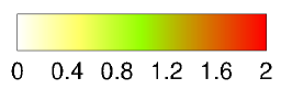
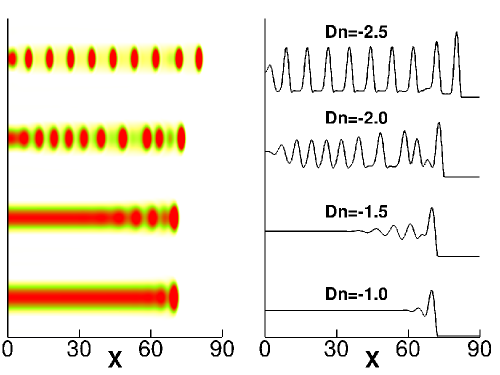
Figure 1: (Color online) Rivulet flow for different $Dn$’s at $t=25$. The domain size is specified by $L=90$ and $M=5$. Left hand side shows the contour plot and the right hand side shows the cross section ($y=\mbox{const}$.) at the middle of a rivulet. We will use similar way of presenting results, and the same color map in the other figures given in this paper.

For $Dn=-1.0$, we still observe traveling type solution. We have examined speed of the capillary ridge and found that it equals $V_{r}$, as predicted. For $Dn$ larger in absolute value, the traveling type solution becomes unstable and waves keep forming right behind the capillary ridge. For $Dn>-1.5$, simulations suggest that the instability is convective, since it is carried by the flow and moves downstream from the initial contact line position, $x_{f}$. For $Dn<-1.5$, the instability is absolute. At the time shown, the whole rivulet is covered by waves which in the cross section resemble solitary ones.

The rivulet simulations show a qualitative similarity to our 2D simulations (vis. the right hand side of Fig. 1 and Fig. 4 in [13]). Therefore, on one hand this result validates the accuracy of our 3D simulations. On the other hand, it also suggests that the instability regimes, (type 1, 2 and 3) can be extended to 3D rivulet geometry. Clearly, it was necessary to use renormalized value of $D$, $Dn$, to be able to carry out this comparison.

It is also of interest to relate the present results to stability properties of an inverted infinite length rivulet without a front. In this case, it is known that there exists a critical angle between $\pi/2$ and $\pi$ such that the inverted infinite rivulet is unstable if the inclination angle is larger than the critical one [29]. In order to be able to directly compare the two problems (with and without a front), we have carried out simulations of an inverted infinite rivulet. The steady state is fixed by choosing $A=2$. We perturb the rivulet at $t=0$ by a single perturbation defined by $h(x,y,0)=h_{r}(y)(1+A_{r}sech(x-x_{p}))$ with $A_{r}=0.2$ and $x_{p}=5.0$. In this work we consider only this type of perturbation and do not discuss in more detail the influence of its properties on the results. For this case, we find that an inverted infinite rivulet is unstable for $Dn\leq-0.74$, which is consistent with the fact that there exists a critical angle for stability [29]. An obvious question to ask is which instability is dominant for sufficiently small $Dn$’s, such that both front-induced and surface-perturbation induced instabilities are present. This question will also appear later in the context of thin film flow - to avoid repetition we consider it for that problem, in Sec. 4.3.

4 Inverted film with a front

We proceed with analyzing stability of an inverted film with a front flowing down a plane. In Sec. 4.1 we extend the results of the linear stability analysis in the transverse direction to the inverted case. Then, we proceed with fully nonlinear time dependent simulations in Sec. 4.2. We start with addressing a simple case where we perturb the fluid front by a single wavelength only – this case allows us to correlate the results with the 2D surface instabilities discussed previously [13], with the instabilities of a single inverted rivulet discussed in Sec. 3, and also with the well known results for transverse instability of a film front flowing down an inclined plane, see e.g. [15]. We proceed with more realistic simulations of a front perturbed by a number of modes with random amplitudes, where all discussed instability mechanisms come into play. To illustrate complex instability evolution, we also include animations of the flow dynamics for few selected cases [31]. We conclude the section by discussing in Sec. 4.3 the connection between the instabilities considered here with Rayleigh-Taylor type of instability of an infinite film flowing down an inverted plane.

4.1 Linear stability analysis in the transverse direction

In order to analyze the stability of the flow in the transverse, $y$, direction, we perform a linear stability analysis (LSA). The results of similar analysis were reported in previous works, see, e.g., [24], but they typically concentrated on the downhill flows, with $D\geq 0$. Here we extend the analysis to also consider films on an inverted surface, with $D<0$.

Consider a moving frame defined by $s=x-Vt$, and assume a solution of the form

$$h(s,y,t)=H(s)+\epsilon h_{1}(s,y,t),$$ (12)

where $\epsilon\ll 1$, $H(s)$ is the traveling wave solution with the speed $V$. Then, plug this ansatz into Eq. (3). The leading order term ($O(\epsilon^{0})$) gives the 2D equation

$$-VH^{\prime}+[H^{3}(H^{\prime\prime\prime}-DH^{\prime}+1)]^{\prime}=0$$ (13)

while the first order term ($O(\epsilon^{1})$) yields

$$\frac{\partial h_{1}}{\partial t} = -\nabla\cdot\left[H^{3}\nabla\nabla^{2}h_{1}+3H^{2}h_{1}\nabla\nabla^{2}H\right]$$ (14)

$$+D\nabla\cdot\left[H^{3}\nabla h_{1}+3H^{2}h_{1}\nabla H\right]$$

$$-\left(3H^{2}h_{1}\right)_{s}+Vh_{1s},$$

where $\nabla=(\partial_{s},\partial_{y})$. The next step is to express the solution, $h_{1}$, as a continuous superposition of Fourier modes,

$$h_{1}(s,y,t)=\int^{0}_{-\infty}\phi(s,q)e^{\sigma t}e^{iqy}dq,$$ (15)

where $q$ is the wavenumber and $\sigma$ is the growth rate that determines the temporal evolution of $h_{1}$. For a given $q$, there is an associated eigenvalue problem, see e..g, [24]. The largest eigenvalue corresponds to the growth rate, which is the quantity of interest.

Figure 2 shows the LSA results. Each curve represents the corresponding largest eigenvalue for a given wavenumber and for fixed $D$. One can see that sufficiently long wavelengths are unstable. Consequently, there is a critical wavenumber, $q_{c}(D)$, which determines the range of unstable wavenumbers to be $[0,q_{c}]$. Concentrating now on negative $D$’s, we find that $q_{c}$ increases with $|D|$, suggesting shorter unstable wavelength for larger $|D|$’s, which are furthermore expected to grow faster. Therefore, for $D<0$, as $|D|$ is increased (for example by increasing the angle $\alpha$, or by making the film thicker), LSA predicts formation of more unstable fingers spaced more densely.

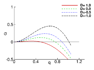
Figure 2: (Color online) Wavenumber, $q$, and corresponding growth rate $\sigma$ for different $D$’s.

One may note that Fig. 2 only shows the results for $D$ down to $-1.0$. The reason is that a base state could be found only for $D\geq-1.1$, and therefore LSA could not be carried out for smaller $D$’s. This issue was discussed in [13], where we were able to find traveling wave solutions only for $D$’s in type 1 regime, and could not find such solutions in type 2 and 3 regimes.

4.2 Fully 3D simulations

In this section we discuss the results of fully 3D simulations of the thin film equation, Eq. (3). Throughout this section as our initial condition we chose the same profile as in 2D simulations [13] - that is, two flat regions of thickness $h=1$ and $h=b$ connected at $x=x_{f}$ by a smooth transition zone described by a hyperbolic tangent, perturbed as follows

$$x_{f}(y)=x_{f0}-A_{0}\cos(2\pi y/\lambda),$$

where $\lambda$ is the wavelength of the perturbation and $x_{f0}$ is the unperturbed position. Here we choose $x_{f0}=5$. The boundary conditions in the flow direction are such that constant flux at the inlet is maintained, while at $x=L$, we assume that the film thickness is equal to the precursor. The boundary conditions implemented here are

$$h(0,y,t)=1,\quad h_{xxx}(0,y,t)-D\,h_{x}(0,y,t)=0,$$

$$h(L,y,t)=b,\quad h_{x}(L,y,t)=0.$$

For the $y$ boundaries, we use the no-flow boundary conditions as

$$h_{y}(x,0,t)=h_{y}(x,M,t)=0,$$ (16)

$$h_{yyy}(x,0,t)=h_{yyy}(x,M,t)=0,$$

where $M$ is the width of the domain in the $y$ direction.

Figure 3 shows the results of simulations for $D=-1.0$ perturbed by specified single mode perturbations. For $\lambda=8$ and $\lambda=10$, the perturbation evolves into a single finger, whereas for $\lambda=20$, which corresponds to the wavelength larger than the most unstable one (vis. Fig. 2), we observe a secondary instability: in addition to the finger that corresponds to the initial perturbation, there is another one (which appears as half fingers at $y=0,M$), developing at later time (in this case after $t=10$). This phenomenon can be explained by the fact that the domain is large enough to allow for two fingers to coexist.

Figure 3: (Color online) Time evolution for perturbations of different wavelengths ($\lambda$) and $D=-1.0$. Here the domain is specified by $L=50$ and $M=\lambda$.

Next, we compare the growth rate of a finger from 3D simulation with the LSA results. This comparison is shown in Fig. 4 for $D=-0.5$ and $D=-1.0$. The initial condition for these simulations is chosen as a single mode perturbation, $\lambda=M=10$. The growth rate is extracted by considering the finger’s length, $A$, defined as the distance between tip and root. As shown in Fig. 4, for early times, the finger grows exponentially with the same growth rate as predicted by the LSA. For later times, the finger length exhibits a linear growth. This late time behavior can be simply explained by the fact that the finger evolves into the rivulet solution discussed in Sec. 3.

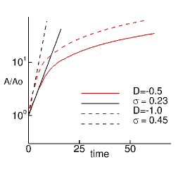
Figure 4: (Color online) Length of a finger, $A$, divided by the initial length, $A_{0}$. Here $\lambda=M=10$. Red (curved) lines show the computational results while the black (straight) lines show the LSA prediction for two different $D$’s.

Figure 5 shows the numerical results for $D=-1.5$ with three single mode perturbations in a fixed domain, $[0,90]\times[0,20]$. Both contour plots and the cross sections at middle of the domain ($y=10$) are presented. In this case, in addition to the secondary instability in the case of the perturbation by $\lambda=20$, we also see secondary instability developing for $\lambda=10$, suggesting that as the absolute value of (negative) $D$ grows, shorter and shorter wavelengths become unstable. For this $D$, even $\lambda=5$ is unstable. This result is consistent with the trend of the LSA results shown in Fig. 2; note however that LSA cannot be carried out for such small $D$’s due to the fact that traveling wave solution could not be found. Instead of traveling waves, we find surface instabilities on the film. As shown in the contour plot at $t=50$, several red(dark) dots, which represent waves, appear on the fingers, as it can be seen in the cross section plots as well. The red(dark) dots keep forming, moving forward and interact with the capillary ridge in the fronts. This interaction can be seen much more clearly in the animations available as supplementary materials [31].

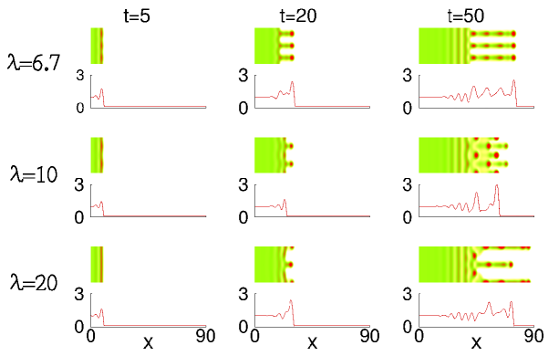
Figure 5: (Color online) Time evolution for perturbations of different wavelengths ($\lambda$) at $D=-1.5$. The domain is chosen as $L=90$ and $M=20$. In each sub-block, the upper figure shows the contour plot, and the lower figure shows the cross section at $y=10$.

The cross section plots in Fig. 5 show formation of solitary-like waves. Behind these solitary-like waves, there exists a second region where waves appear as ‘stripes’ (vis. the straight stripes in the middle part of the contour plot at $t=50$). These stripe-waves move forward for a short distance and then break into several waves localized on the surface of the finger-like rivulets. In the cross-section plots, these strip-like waves appear as sinusoidal waves. Finally, flat film is observed in the region far behind the contact line. The appearance of such a flat film indicates that the flow instability is of convective type. Therefore, for this $D$, the contact line induced waves are carried by the fluid and they eventually move away from any fixed position.

Figure 6 shows the numerical results for $D=-2.0$ with the same set of initial perturbation as in Fig. 5. Both contour plot and the cross sections at the middle of the $y$ domain are presented. As mentioned in [13], $D=-2.0$ corresponds to the Type 2 regime and is of absolute instability type. This is exactly what we see in the contour plot. Localized waves shown as red (dark) dots appear all over the surface and we do not see neither strip waves nor flat film appearing. In the cross section plots, we only see solitary-like waves.

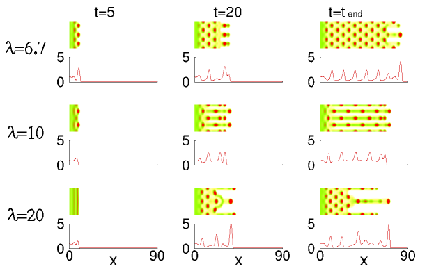
Figure 6: (Color online) Time evolution for perturbations of different wavelengths ($\lambda$) at $D=-2.0$. $t_{end}=50$ for $\lambda=6.67$, $t_{end}=40$ for $\lambda=10$, $t_{end}=30$ for $\lambda=20$. The domain is chosen as $L=90$ and $M=20$. In each sub-block, the upper figure shows the contour plot, and the lower figure shows the cross section at $y=10$.

Next we proceed to analyze the behavior in the case where initially multiple perturbations are present. The imposed perturbation consists of $50$ sinusoidal modes with amplitudes randomly selected from $[-0.2,0.2]$

$$x_{f}(y)=x_{f0}-\sum_{i=1}^{50}\,A_{i}\,\cos((i-1)\,\pi\,y),\quad-0.2\leq A_{i}\leq 0.2\,.$$

Figure 7 shows the simulations for different $D$’s with the same random initial perturbations. The initial profile is shown in Fig. 7 ($t=0$). The initial condition is set to be the same for all $D$’s so that the non-dimensional parameter $D$ is the only difference between the 4 panels in Fig. 7.

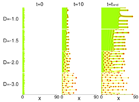
Figure 7: (Color online) Time evolution of perturbations for different $D$’s with the same random initial perturbations. Here $t_{end}=50$ for $D=-1.0$, $t_{end}=40$ for $D=-1.5$, $t_{end}=30$ for $D=-2.0$, $t_{end}=20$ for $D=-3.0$. The domain is chosen as $L=90$ and $M=50$ See also the animations available [31].

The first obvious observation is that the number of fingers increases as the absolute value of (negative) $D$ becomes larger. This is due to the fact that the most unstable wavelength decreases as $|D|$ of (negative) $D$ becomes larger. Therefore more fingers can fit into the flow domain. Secondly, the fingers become more narrow for these $D$’s, consistently with the predictions for rivulet flow. Thirdly, the absolute/convective instability argument in [13] is a good explanation for these contact line induced instabilities: there is no surface instability seen for $D=-1.0$; we see convective instability, shown as localized waves/stripes/flat film for $D=-1.5$; and absolute instability for $D=-2.0$ and $D=-3.0$.

Remark

Here we comment on two additional sets of simulations - corresponding figures are omitted for brevity. One set involves the case when the initial condition is chosen as $y$-independent. Mathematically such initial condition reduces the problem to 2D, and the solution should remain $y$-independent for all times. However, this is not the case in numerical simulations. Numerical errors are present and grow with time. To estimate this effect, one can calculate the largest grows rate in the $x$ and $y$ direction based on the LSA results, and estimate the time for which the numerical noise becomes significant. For example, for $D=-1.0$, the largest growth rate for instability of a flat film in the $x$ direction is $0.25$ and the largest growth rate in the $y$ direction is $0.46$. That is, it takes $70$ time units for noise of initial amplitude $10^{-16}$ (typical for double precision computer arithmetic) to grow to $10^{-2}$. So as long as the final time is less than $70$, the numerical noise is still not visible. By carrying out such an analysis, we are able to distinguish between the numerical noise induced instability and the contact line induced one, and further separate the effect of numerical noise.

The other set or simulations has to do with the case when the initial single mode perturbation is chosen as a stable one. In such a case, the amplitude of perturbation decays exponentially and the surface profile soon becomes $y$-independent. Again, after sufficiently long time, numerical noise will become relevant and break the $y$-independence.

4.2.1 The width of a finger

It is of interest to discuss how fingers’ width depend on $D$. As a reminder, the LSA shows that there exists a most unstable wavenumber, $q_{m}(D)$, and the distance between two neighboring fingers in physical experiments, in the presence of natural or other noise, is expected to center around the most unstable wavelength, $\lambda_{m}=2\pi/q_{m}(D)$. On the other hand, the width of the rivulet part of a single finger is not known to the best of our knowledge. In the following we define this width and discuss how it relates to the LSA results.

First we check whether there is a difference between the fingers for different single mode perturbations. Figure 8 shows the $y$-orientation cross section of the fingers’ rivulet part for $D=-0.5$ and $D=-1.0$. As shown in the figure, for a given $D$, the fingers are very similar in the cross section, with their shape almost independent of the initial perturbation. Note that this result still holds even for the $\lambda$’s that are very close to the critical one, $\lambda_{c}={2\pi/q_{c}(D)}$ - eg., see $\lambda=6.3$ in Fig. 8(b) (here $\lambda_{c}\approx 6.25$). By direct comparison of the parts (a) and (b) of this figure, we immediately observe that the fingers are more narrow for more negative $D$’s.

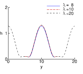
(a) $D=-0.5$.

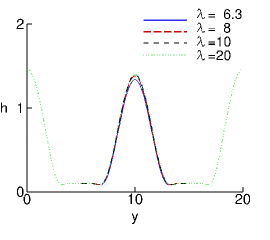
(b) $D=-1.0$.

Figure 8: (Color online) Cross sections of film thickness as a function of the transverse coordinate, $y$, for different wavelengths of initial perturbation, $\lambda$. The cross sections are taken from the rivulet part of a finger, at $x=35$, $t=30$; some of results from which the cross sections are extracted can be seen in Fig. 3. The centers of the cross sections are shifted to $y=10$ for the purpose of comparison. For $D=-0.5$, $\lambda=6.3$ is stable (not shown).

To make this discussion more precise, we define the width of a rivulet, $w$, as the distance between two dips on each side of a finger (the two dips are shown at $y\approx 7$ and $y\approx 13$ in Fig. 8). The main finding is that $w\approx\lambda_{c}$. This finding applies for all $D$’s and all perturbation wavelengths that we considered. In particular note that Fig. 8 shows that $w$ becomes smaller as absolute value of (negative) $D$ increases, consistently with the decrease of $\lambda_{c}$, see Fig 2.

While it is clear that $w$ can not be larger than $\lambda_{c}$ (since $w$ is independent of the initial perturbation, and for $\lambda>\lambda_{c}$ it must be that $\lambda>w$), at this point we do not have a precise argument why $w$ is so close to $\lambda_{c}$ for all considered perturbations and the values of $D$. Of course, one could argue that $w\approx\lambda_{c}$ is also consistent with stability of any perturbation characterized by $\lambda<\lambda_{c}$, since such a perturbation cannot support a finger of $w\approx\lambda_{c}$.

4.3 Rayleigh-Taylor instability of inverted film

The instabilities we have discussed so far are discussed in the fluid configurations where contact line is present, and an obvious question is what happens if there is no contact line, that is, if we have an infinite film spreading down an (inverted) surface. This configuration is expected to be susceptible to Rayleigh-Taylor (R-T) type of instability since we effectively have a heavier fluid (liquid) above the lighter one (air). The question is what are the properties of this instability for a film flowing down an inverted surface, and how this instability relates to the contact line induced one, discussed so far.

Figure 9 shows the results of 3D simulation of an infinite film (no contact line). The initial condition at $t=0$ is chosen as a flat film with localized half-sphere-like perturbation of amplitude $0.1$ (marked by the black circle in Fig. 9). As an example, we use $D=-1.0$. At time $t=20$, the perturbation had been amplified, as expected. The properties of this instability are, however, very different from the one observed in thin film flow where contact line is present. For this $D$, if a contact line is present, we see only a capillary wave behind the front (vis. Fig. 3 and Fig. 7), and we do not find upstream propagating waves as for the infinite film shown in Fig. 9. Therefore, the instability discussed so far is not of R-T type - instead, it is induced by the presence of a contact line.

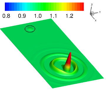
Figure 9: (Color online) Simulation of Rayleigh-Taylor instability for hanging film on inclined plane at $D=-1.0$. The black circle indicates the initial profile. The surface shown in the downstream is the surface profile at $t=20$. The computational domain is $[0,90]\times[0,50]$.

One obvious question is why we do not observe (additional) R-T instability in the flow with fronts. The answer is that the speed with which a perturbation on a main body of a film (such as infinite film shown in Fig. 9) propagates downstream is faster than the speed of the contact line itself. Therefore, in the simulations of films with fronts presented so far, flat film instabilities do not have time to develop since they reach the contact line before having a chance to grow. We note that in Fig. 9 we used large scale perturbation to illustrate the point; in a physical problem, one would expect surface perturbations to be characterized by much smaller amplitudes and would therefore require much longer time to grow to the scale comparable to the film thickness. As a consequence, R-T instability could be expected to become relevant only for the films characterized by the spatial extend which is much larger than the one considered here. Similar conclusion extends to stability of infinite rivulets, discussed briefly in Sec. 3.

5 Inverted film of variable viscosity with a front

Consider now a situation, when the film is of finite width and the fluid viscosity is variable in the transverse direction, ie., $\bar{\mu}=\bar{\mu}(y)$ in Eq. (3). We have to substitute the no-flow boundary conditions, Eq. (16), at the borders of the computational domain with the following ones

$$h(x,0,t)=h(0,M,t)=b,$$

$$h_{x}(x,0,t)=h_{x}(0,M,t)=0,$$

The flow starts at the top of the domain according to the condition

$$h(0,y,t)=b+F_{0}\left(\frac{y}{M}\right)\frac{(at)^{2}}{1+(at)^{2}},$$ (17)

where the value of parameter $a$ is $0.775$ and the bell shape of the entrance thickness profile determined by the function $F_{0}$ is shown in Fig. 10. Equation (17) mimics the growth of the flow rate and the film thickness at the entrance boundary as the liquid starts being delivered to the substrate during the ramp-up in industrial processes or experiments. Characteristic patterns of flow depend on the value of parameter $D$, width of the film and distribution of viscosity, and establish when the product $at$ in Eq. (17) reaches values of several units.

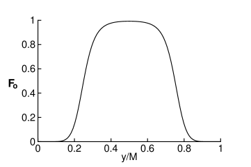
Figure 10: Entrance profile of film thickness.

In many practical situations, the variation of viscosity is a result of its dependence on temperature, which is usually non-linear. For example, assume that the film temperature $T$ drops linearly with the lateral coordinate $y$ and the viscosity (in $Pa\cdot s$) is given by a generic equation:

$$T = T_{0}-ay,\quad a=\mbox{const.};$$ (18)

$$\log_{10}(\mu) = -A+\frac{B}{T-C},$$ (19)

where $A=5.5$, $B=700$ K and $C=52$ K are the material constants, and $T$ is the liquid temperature. The viscosity function is normalized by its value at $y=0$. The constant value $T_{0}$ is assumed to be equal $153$ K, while the lateral temperature drop across the computational domain is assumed to be equal $11$ K in all cases discussed hereafter, resulting in $7.5$ fold viscosity growth from bottom to top of the domain.

Similarly to isoviscous cases discussed earlier, the film front is always unstable, producing finger-like rivulets. The morphology of the non-isoviscous film (as compared to an isoviscous case) stems from the fact that similar structures such as fingers at different parts of the film move with different speeds. As an example, Fig. 11 (a) and (b) show distribution of film thickness at $t=9.4$, $16.5$, with parameter $D=-0.88$ and the dimensionless domain width $M$ equal to $133$. Morphology of individual fingers is similar to the one of fingers in isoviscous cases shown in Fig. 7, but there is obvious mass redistribution along the front line because of its inclination, resulting in coalescence of some of the fingers and variation of the finger-to-finger distance. A finger produced by coalescence of two parent fingers, such as finger $5$ in Fig. 11(b), has a higher flow rate and moves faster than its neighbors.

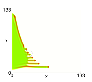
(a) $t=9.4$.

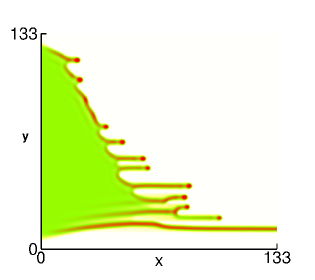
(b) $t=16.5$.

Figure 11: (Color online) Film thickness for $D=-0.88$. The circle in the part (a) indicates two coalescing fingers.

These specific properties of non-isoviscous film are common for flows in the whole spectrum of parameter $D$, but morphology of individual fingers strongly depends on the type of the flow, similar to already considered isoviscous cases. Figure 12 shows distribution of film thickness for parameter $D=-1.5$, which corresponding to type 2, with film width $M=72.2$, at $t=25.4$. The leading head capillary ridges are followed by a rivulet with followup smaller waves moving faster than the leader. The pattern is common for all fingers, but the speed of propagation increases with temperature. Each of the fingers has a faster-moving neighbor on the higher temperature side, causing slight increase of the background film thickness on that side compared to the colder side. As a result, the fingers may have a tendency of being diverted and coalesce with warmer neighbors resulting in mass transport from colder areas to warmer areas of the flow, despite the fact that the film velocity does not explicitly depend on the temperature gradient.

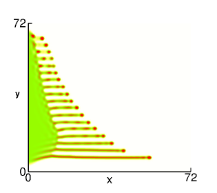
Figure 12: (Color online) Film thickness for $D=-1.5$ at $t=25.4$.

In type 3 film flow, the height of follow-up drops is already close to that of finger head drops, as shown in Fig. 13, showing thickness distribution in film with parameter $D=-2.54$, film width $M=52.2$ at $t=44.4$. In type 3 flows, there is no propagation front and the flow itself consists of a series of propagating fingers. Another peculiarity of this type of flows is existence of small drops, separating from the leading drops to be immediately consumed by the following drop in the train, as indicated by circles in Fig. 13. These features are also observed in isoviscous flows for similar values of $D$; see, e.g., cross sectional profile in Fig. 6. The viscosity effect in the developed type 3 flows shows mainly as the difference in speeds for droplets in low and high viscosity regions.

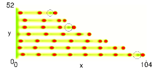
Figure 13: (Color online) Film thickness for $D=-2.54$ at $t=44.4$.

6 Conclusions

In the previous work [13] we carried out extensive computational and asymptotic analysis of the two dimensional flow of a completely wetting fluid down an inverted surface. Complex behavior was uncovered with different families of waves evolving in the configurations characterizing by different values of the governing parameter $D$. In the present work, we have considered fully three dimensional problem of spreading down an inverted surface. We find that there is an elaborate interaction of surface instabilities and contact line instabilities. For the values of $D$ which are not too small (approximately $D\geq-1.1$) we find similar behavior as already known for the flow down an inclined surface, with the main difference that the finger-like patterns that form are spaced more closely and the fingers themselves are more narrow for negative $D$’s. As $D$ is further decreased, we still find instabilities of the contact line leading to formation of fingers, but in addition we observe formation of surface waves, which propagate down the fingers with the speed larger than the speed of the fingers themselves: therefore, these propagation waves (which may appear as drops on top of the base film) travel down a finger, reach the front and merge with the leading capillary ridge. Behind the fingers, in this regime we find strip-like waves (whose fronts are independent of the transverse direction). These waves are convective in nature and leave behind a portion of a flat film whose length increases with time. For even smaller $D$’s (smaller than approximately $-2.0$), these transverse strip-like waves disappear, and the whole film is covered by localized waves. These localized waves travel faster than the film itself, and converge towards the fingers which form at the front.

It is worth emphasizing that the properties of the surface waves which form due to the presence of fronts are different from the ones which would be expected if the fronts were not present. To illustrate this effect, we consider an infinite film with a localized perturbation which is expected to be unstable by a Rayleigh-Taylor type of instability. We find that this instability leads to a different type of surface waves, which may or may not be observable in physical experiments, depending on the size of the fluid domain.

In the second part of the paper we consider flow where fluid viscosity is not constant, but varies in the transverse direction. The most important difference is the loss of flow periodicity in the lateral direction. The fingers in the warmer parts of the flow move faster than those in the colder areas, yielding slight increase of the background film thickness on warmer side of each finger compared to the colder side. This results in mass redistribution from colder areas to warmer areas of the flow, more pronounced for lower values of $|D|$, despite explicit independence of the film velocity on the temperature gradient.

Acknowledgments. This work was partially supported by NSF grant No. DMS-0908158.

Appendix A Numerical method for 3D thin film equation

A.1 Solving nonlinear time dependent PDE

In general, time dependent PDE, Eq. (3), can be expressed as $h_{t}+f(h)=0$, where $h=h(\mbox{\boldmath$x$},t)$ is the unknown function with time variable $t$, spatial variables $x$, and $f$ is a nonlinear discretization operator for spatial variables. From time $t^{n}=n\Delta t$ to $t^{n+1}$, where $\Delta t$ is the time step, the PDE can be integrated numerically by the so-called $\theta$ method leading to a nonlinear system:

$$h^{n+1}+(1-\theta)\Delta tf^{n+1}=h^{n}-\theta\Delta tf^{n},$$ (20)

where $f^{n}=f(h^{n})$ and $h^{n}=h(\mbox{\boldmath$x$},t^{n})$. To solve the nonlinear system (20), we apply the Newton’s method. Firstly, we linearize $h^{n+1}$ about a guess for the solution by assuming $h^{n+1}=h^{*}+c$, where $h^{*}$ is a guess and $c$ is the correction. Then we express the nonlinear part using Taylor’s expansion

$$f^{n+1}=f(h^{*}+c)\approx f(h^{*})+J_{f}(h^{*})\cdot c=f^{*}+J_{f}^{*}\cdot c,$$

where $J_{f}$ is the Jacobian matrix for function $f$ and $J_{f}^{*}=J_{f}(h^{*})$. After substituting the above quantities into Eq. (20), we obtain a linear system for the correction term, $c$:

$$\left(I+(1-\theta)\Delta tJ_{f}^{*}\right)c=-h^{*}-(1-\theta)\Delta tf^{*}+h^{n}-\theta\Delta tf^{n},$$ (21)

$I$ is the identity matrix that has the same size as the Jacobian matrix, $J^{*}_{f}$. The solution at $t=t^{n+1}$ is obtained by correcting the guess iteratively until the process converges, ie., the new correction is small enough.

A.2 Spatial discretization

We discretize the spatial derivatives of thin film equation, Eq. (3), through finite difference method. The grid points in the computational domain, $[0,L]\times[0,M]$, is defined as

$$x_{i} = \left(i-\frac{1}{2}\right)\Delta x,\quad i=1,\cdots,n_{x},$$

$$y_{j} = \left(j-\frac{1}{2}\right)\Delta y,\quad j=1,\cdots,n_{y},$$

where $\Delta x=L/n_{x}$, $\Delta y=M/n_{y}$ are the step size in the $x$, $y$ domain; $n_{x}$, $n_{y}$ are number of grid points in the $x$, $y$ domain, respectively.

The scheme presented here is 2nd order central difference scheme. In the following, the subscripts, $i,j$, denote that the value been taken at $(x_{i},y_{j})$. The notation $h_{i+1/2,j}$ denotes an average at the point $(x_{i+1/2},y_{j})$ as

$$h_{i+1/2,j}=\frac{h_{i+1,j}+h_{i,j}}{2}.$$

Also we use the standard difference notation as

$$\delta_{x}h_{i+1/2,j} = h_{i+1,j}-h_{i,j},$$

$$\delta_{y}h_{i,j+1/2} = h_{i,j+1}-h_{i,j},$$

$$\delta^{3}_{x}h_{i+1/2,j} = h_{i+2,j}-3h_{i+1,j}+3h_{i,j}-h_{i-1,j},$$

$$\delta^{3}_{y}h_{i,j+1/2} = h_{i,j+2}-3h_{i,j+1}+3h_{i,j}-h_{i,j-1},$$

$$\delta_{x}\delta^{2}_{y}h_{i+1/2,j} = h_{i+1,j+1}-2h_{i+1,j}+h_{i+1,j-1}$$

$$-h_{i,j+1}+2h_{i,j}-h_{i,j-1},$$

$$\delta_{y}\delta^{2}_{x}h_{i,j+1/2} = h_{i+1,j+1}-2h_{i,j+1}+h_{i-1,j+1}$$

$$-h_{i+1,j}+2h_{i,j}-h_{i-1,j}.$$

The discretization of each term in Eq. (3) involving spatial derivatives is as follows:
The surface tension term

$$\nabla\cdot[h^{3}\,\nabla\nabla^{2}h]_{i,j}=$$

$$\left(h^{3}_{i+1/2,j}\delta^{3}_{x}h_{i+1/2,j}-h^{3}_{i-1/2,j}\delta^{3}_{x}h_{i-1/2,j}\right)/\Delta x^{4}$$

$$\left(h^{3}_{i+1/2,j}\delta_{x}\delta^{2}_{y}h_{i+1/2,j}-h^{3}_{i-1/2,j}\delta_{x}\delta^{2}_{y}h_{i-1/2,j}\right)/\Delta x^{2}\Delta y^{2}$$

$$\left(h^{3}_{i,j+1/2}\delta_{y}\delta^{2}_{x}h_{i,j+1/2}-h^{3}_{i,j-1/2}\delta_{y}\delta^{2}_{x}h_{i,j-1/2}\right)/\Delta x^{2}\Delta y^{2}$$

$$\left(h^{3}_{i,j+1/2}\delta^{3}_{y}h_{i,j+1/2}-h^{3}_{i,j-1/2}\delta^{3}_{y}h_{i,j-1/2}\right)/\Delta y^{4}.$$

The normal gravity term

$$\nabla\cdot[h^{3}\,\nabla h]_{i,j}=$$

$$\left(h^{3}_{i+1/2,j}\delta_{x}h_{i+1/2,j}-h^{3}_{i-1/2,j}\delta_{x}h_{i-1/2,j}\right)/\Delta x^{2}$$

$$+\left(h^{3}_{i,j+1/2}(h_{i,j+1}-h_{i,j})-h^{3}_{i,j-1/2}(h_{i,j}-h_{i,j-1})\right)/\Delta y^{2}.$$

The tangential gravity term

$$\frac{\partial}{\partial x}\left(h^{3}\right)_{i,j}=\left(h^{3}_{i+1/2,j}-h^{3}_{i-1/2,j}\right)/\Delta x.$$ (22)

A.3 Fully implicit algorithm

Applying algorithm Eq. (21) to 3D thin film Eq. (3), we have [32]

$$\left(I+(1-\theta)\Delta t(J_{fx}^{*}+J_{fy}^{*}+J_{fm}^{*})\right)\cdot c=$$

$$-h^{*}-(1-\theta)\Delta tf^{*}+h^{n}-\theta\Delta tf^{n},$$ (23)

where $J_{fx}$, $J_{fy}$ and $J_{fm}$ are the Jacobian matrices for $x$, $y$ and mixed derivative terms of function $f$, respectively. Equation (23) is a non-symmetric sparse linear system that has $n_{x}n_{y}$ unknowns. For large $n_{x}$ and $n_{y}$, as it is the case for the problems discussed in the present work, solving such a system carries a significant computational cost. In general, the operation count is proportional to $O(n_{x}^{3}n_{y}^{3})$ or $O(n_{x}^{2}n_{y}^{2})$, depending on the matrix solver.

A.4 ADI method

To decrease the computational cost, Witelski and Bowen suggested to use the approximate-Newton approach [33]. The idea is to replace the Jacobian matrix by an approximated one

$$\left[I+(1-\theta)\Delta t\left(J^{*}_{fx}+J_{fy}^{*}+J_{fm}^{*}\right)\right]$$ (24)

$$\sim\left[I+(1-\theta)\Delta tJ^{*}_{fy}\right]\left[I+(1-\theta)\Delta tJ^{*}_{fx}\right]$$ .

Therefore we get a new system of equations

$$\left[I+(1-\theta)\Delta tJ^{*}_{fy}\right]\left[I+(1-\theta)\Delta tJ^{*}_{fx}\right]\cdot c=R,$$ (25)

where $R=-h^{*}-(1-\theta)\Delta tf^{*}+h^{n}-\theta\Delta tf^{n}$ is the right hand side of Eq. (23). One should note that as long as $c$ decreases after each iteration and approaches $0$ in some norm, we have $R=0$, leading to Eq. (20). That is, such an approach does not affect the stability and accuracy of the original space-time discretization.

Under the same spirit of alternating direction implicit method (ADI), equation (25) can be easily split into two steps:

$$\left(I+(1-\theta)\Delta tJ_{fx}^{*}\right)\cdot w = R,$$

$$\left(I+(1-\theta)\Delta tJ_{fy}^{*}\right)\cdot c = w.$$ (26)

The main advantage of such splitting is that the operations in the $x$ and $y$ directions are decoupled and therefore the computational cost reduced significantly. Specifically for our discretization, the Jacobian matrices in the $x$ and $y$ direction are penta-diagonal matrices, leading to system that can be solved in $O(n_{x})$ and $O(n_{y})$ arithmetic, and the overall computational cost for solving Eq. (26) is proportional to $O(n_{x}n_{y})$.

The approach presented here deals with a matrix that is an approximation to the original Jacobian one. Therefore we should not expect the convergent rate of the ADI method to be quadratic. However, since the approximation error is proportional to $O(\Delta t)$, for small enough time step, we expect the rate of convergence to be close to quadratic; see [33] for further discussion of this issue. Furthermore, the ratio in the operation count between fully implicit discretization and the ADI method is $O(n_{x}n_{y})$. That is, even if we need to decrease the time step or increase the number of iterations to achieve convergence, the ADI method is still more efficient as long as the additional effort is of $o(n_{x}n_{y})$. In our experience, under the same conditions, ADI method is significantly more efficient compared to fully implicit discretization.

References

- [1] K.J. Ruschak. Coating flows. Ann. Rev. Fluid Mech., 17:65, 1999.
- [2] H.-C. Chang and E. A. Demekhin. Complex wave dynamics on thin films. Elsevier, New York, 2002.
- [3] A. Oron, S. H. Davis, and S. G. Bankoff. Long-scale evolution of thin liquid films. Rev. Mod. Phys., 69:931, 1997.
- [4] H.A. Stone, A.D. Stroock, and A. Ajdari. Engineering flows in small devices. Ann. Rev. Fluid Mech., 36:381, 2004.
- [5] R. V. Craster and O. K. Matar. Dynamics and stability of thin liquid films. Rev. Mod. Phys., 81:1131, 2009.
- [6] P. L. Kapitsa and S. P. Kapitsa. Wave flow of thin fluid layers of liquid. Zh. Eksp. Teor. Fiz., 19:105, 1949.
- [7] J. Liu and J. P. Gollub. Onset of spatially chaotic waves on flowing films. Phys. Rev. Lett., 70:2289, 1993.
- [8] S. V. Alekseenko, V. E. Nakoryakov, and B. G. Pokusaev. Wave flow of liquid films. Begell House, New York, 1994.
- [9] H.-C. Chang. Wave evolution on a falling film. Annu. Rev. Fluid Mech., 26:103, 1994.
- [10] S. Saprykin, E. A. Demekhin, and S. Kalliadasis. Two-dimensional wave dynamics in thin films. I. Stationary solitary pulses. Phys. Fluids, 17:117105, 2005.
- [11] Y. Y. Trifonov and O. Y. Tsvelodub. Nonlinear waves on the surface of a falling liquid film. part 1. waves of the first family and their stability. J. Fluid Mech., 229:531, 1991.
- [12] H.-C. Chang, E. A. Demekhin, and S. S. Saprikin. Noise-driven wave transitions on a vertically falling film. J. Fluid Mech., 462:255, 2002.
- [13] T.-S. Lin and L. Kondic. Thin film flowing down inverted substrates: two dimensional flow. Phys. Fluids, 22:052105, 2010.
- [14] S. M. Troian, E. Herbolzheimer, S. A. Safran, and J. F. Joanny. Fingering instabilities of driven spreading films. Europhys. Lett., 10:25, 1989.
- [15] J. A. Diez and L. Kondic. Contact line instabilities of thin liquid films. Phys. Rev. Lett., 86:632, 2001.
- [16] L. Kondic and J. A. Diez. Contact line instabilities of thin film flows: Constant flux configuration. Phys. Fluids, 13:3168, 2001.
- [17] H. E. Huppert. Flow and instability of a viscous current down a slope. Nature, 300:427, 1982.
- [18] N. Silvi and E. B. Dussan V. On the rewetting of an inclined solid surface by a liquid. Phys. Fluids, 28:5, 1985.
- [19] J. R. de Bruyn. Growth of fingers at a driven three–phase contact line. Phys. Rev. A, 46:4500, 1992.
- [20] S. V. Alekseenko, D. M. Markovich, and S. I. Shtork. Wave flow of rivulets on the outer surface of an inclined cylinder. Phys. Fluids, 8:3288, 1996.
- [21] A. Indeikina, I. Veretennikov, and H.-C. Chang. Drop fall-off from pendent rivulets. J. Fluid Mech., 338:173, 1997.
- [22] T.M. Segin, B. S. Tilley, and L. Kondic. On undercompresive shocks and flooding in countercurrent two-layer flows. J. Fluid Mech., 532:217, 2005.
- [23] M. Mavromoustaki, O.K. Matar, and R.V. Craster. Shock-wave solutions in two-layer channel flow. I. One-dimensional flows. Phys. Fluids, 22:112102, 2010.
- [24] L. Kondic. Instabilities in gravity driven flow of thin liquid films. SIAM Review, 45:95, 2003.
- [25] L. W. Schwartz. Viscous flows down an inclined plane: instability and finger formation. Phys. Fluids A, 1:443, 1989.
- [26] A. Oron and P. Rosenau. Formation of patterns induced by thermocapillarity and gravity. J. Phys. (France), 2:131, 1992.
- [27] A. J. Tanasijczuk, C. A. Perazzo, and J. Gratton. Navier-Stokes solutions for steady parallel-sided pendent rivulets. Euro. J. Mech. B/Fluids, 29:465, 2010.
- [28] J.S. Sullivan, S.K. Wilson, and B.R. Duffy. A thin rivulet of perfectly wetting fluid subject to a longitudinal surface shear stress. Quart. J. Mech. Appl. Math., 61:25, 2008.
- [29] E.S. Benilov. On the stability of shallow rivulets. J. Fluid Mech., 636:455, 2009.
- [30] B.R. Duffy and S.K. Wilson. A rivulet of perfectly wetting fluid with temperature-dependent viscosity draining down a uniformly heated or cooled slowly varying substrate. Phys. Fluids, 15:3236, 2003.
- [31] See supplementary material at [url will be inserted by aip].
- [32] J. A. Diez and L. Kondic. Computing three-dimensional thin film flows including contact lines. J. Comp. Phys., 183:274, 2002.
- [33] T. P. Witelski and M. Bowen. ADI schemes for higher-order nonlinear diffusion equations. Applied Numer. Math., 45:331, 2003.