Pairwise Quantum Correlations for Superpositions of Dicke States

Abstract

Pairwise correlation is really an important property for multi-qubit states. For the two-qubit X states extracted from Dicke states and their superposition states, we obtain a compact expression of the quantum discord by numerical check. We then apply the expression to discuss the quantum correlation of the reduced two-qubit states of Dicke states and their superpositions, and the results are compared with those obtained by entanglement of formation, which is a quantum entanglement measure.

,

1 Introduction

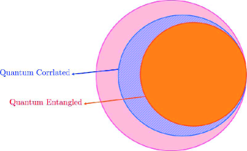
Figure 1: (Color online) Schematic configuration of the relations between quantum correlation and quantum entanglement. The pink circle represents the whole set of quantum states. They can be split into quantum correlated ones (the blue circle) and classical correlated ones. They can also be divided into quantum entangled ones (the red circle) and quantum separable ones. In general, the states with quantum entanglement must be quantum correlated. However, a quantum correlated state may not be quantum entangled. That is, there exists a class of quantum separable states which are also quantum correlated, as shown by the shadow area.

It is well known that quantum entanglement is a typical quantum computation resource and plays an important role in quantum information processing  [1, 2]. Much attention has been paid to detect and measure the quantum entanglement (see  [3, 4, 5] and references therein). Traditionally, it is believed that quantum entanglement is synonymous with quantum correlation. However, it is not always the case. Many works showed that there exists a more general quantum correlation [6, 7, 8, 9] besides entanglement, as shown in figure 1. That is, some separable states can also possess quantum correlation, which can improve some computational tasks [10]. Such the general quantum correlation is quantitatively characterized by quantum discord (QD) [11, 12, 13, 14], which is defined from the quantum measurement perspective. Using this quantity, it was proved that almost all quantum states actually have quantum correlations [15]. Most recently, operational interpretations of quantum discord were proposed, where quantum discord was shown to be a quantitative measure about the performance in quantum state merging [16, 17]. Up to now, QD has been widely studied in many fields[18, 19, 20, 21, 22, 23, 24, 25, 26, 27, 28, 29, 30, 31, 32, 33, 34, 35, 36, 37, 38, 39, 40, 41, 42].

Calculating QD involves an optimization process over all possible quantum measurements. So far, a general analytical expression of QD still lacks even for the two-qubit states. Some analytical results were shown only for a special subset of two-qubit X-states [11, 13, 20, 27, 28, 32]. In this article, we consider a kind of two-qubit X-states with exchange and parity symmetries, whose off-diagonal elements are complex, as shown in equation (11). We give an upper bound for the expression of QD. We find that the expression does not depend on the arguments of the complex off-diagonal elements.

A typical example of the two-qubit X states shown in equation (11) is the reduced two-qubit states of Dicke states and their superposition states. Two motivations inspire us to study the pairwise (or two-qubit) quantum correlation properties of such kinds of states. One comes from the experimental perspective. Dicke states are fundamental multiqubit states. They can be realized both in atomic systems [43, 44] and in photonic systems ([45] and references therein). Many multi-qubit states are based on them, such as W states [46, 47], GHZ states [48] and spin coherent states (SCSs) [49, 50], etc. The importance of the Dicke states in experiment has attracted much theoretical studies [51, 52]. Here we would like to examine their pairwise quantum correlation properties in terms of QD. The other motivation comes from the theoretical aspect. The exchange symmetry of a Dicke state ensures that its two-qubit reduced state can be extracted randomly from the global state. That is, the reduced state of the $i$-th and $j$-th qubits $\rho_{ij}={\rm{Tr}}_{\overline{{ij}}}(\rho_{\rm{global}})$ is invariant for arbitrary positions of $i$ and $j$. Once the two-qubit reduced state $\rho_{{ij}}$ is quantum correlated, all of its possible two-qubit states are quantum correlated. Therefore, to some extent, the existence of the two-qubit quantum correlation sufficiently reflects the multi-qubit quantum correlation. Substantial efforts have been made to quantify multi-qubit quantum correlation in terms of its pairwise correlations [22, 23, 38, 39, 53, 54, 55, 56]. All theses works show that pairwise correlation is really an important property for multi-qubit states.

This paper is organized as follows. In Sec. 2, we give the basic concepts of QD and EoF. The latter is a quantum entanglement measure. In Sec. 3, for the two-qubit X states with exchange and parity symmetries, whose off-diagonal elements are complex, an upper bound of QD is analytically derived. In Sec. 4, we make a comparison between the pairwise QD (PQD) and pairwise EoF (PEoF) for Dicke states and their superposition states.

2 Quantum Correlations

2.1 Quantum discord

In classical information, the mutual information measures the correlation between two random variables $A$ and $B$

$$\mathcal{I}_{c}(A:B)=H(A)+H(B)-H(AB),$$ (1)

where $H(X)=-\sum_{x}p_{x}\log_{2}p_{x}$ are the Shannon entropies for the variable $X(X=A,B)$ and $H(A,B)=-\sum_{a,b}p_{a,b}\log_{2}p_{a,b}$ is the joint system $AB$, $p_{a,b}$ is the joint probability of the variables $A$ and $B$ assuming the values $a$ and $b$, respectively, and $p_{a}=\sum_{b}p_{a,b}(p_{b}=\sum_{a}p_{a,b})$ is the marginal probability of the variable $A(B)$ assuming the value $a(b)$ [57]. The classical mutual information can also be expressed in terms of the conditional entropy as

$$\mathcal{J}_{c}(A:B)=H(A)-H(A|B),$$ (2)

where $H(A|B)=\sum_{a,b}p_{a,b}\log_{2}p_{a|b}$ is the conditional entropy of the variable $A$ given that variable $B$ is known, and $p_{a|b}=p_{a,b}/p_{b}$ is the conditional probability.

In quantum information, to obtain a quantum version of Eq.(2), Ollivier and Zurek employed a complete set of perfect orthogonal projective measurements $\{\Pi_{k}^{B}\}$ with $\sum_{k}\Pi_{k}^{B}=I_{B}$ on the subsystem $B$. The reduced state of subsystem $B$ after the measurement is given as $\rho_{A|\Pi_{k}^{B}}=\frac{1}{p_{k}}\mathrm{Tr}_{B}\left[(I^{A}\otimes\Pi_{k}^{B})\rho^{AB}(I^{A}\otimes\Pi_{k}^{B})\right]$, where $p_{k}=\mathrm{Tr}_{AB}(I_{A}\otimes\Pi_{k}^{B}\rho^{AB})$ is probability for the measurement of the $k$th state in the subsystem $B$. Then, for a known subsystem $B$, one can define conditional entropy of subsystem $A$, $S_{\{\Pi_{k}^{B}\}}(\rho_{A|B}):=\sum_{k}p_{k}S(\rho_{A|\Pi_{k}^{B}})$. Then, for a bipartite quantum state $\rho^{AB}$, the quantum analogues for Eqs.(1) and (2) are given as

$$\mathcal{I}(\rho^{AB})=S(\rho^{A})+S(\rho^{B})-S(\rho^{AB}),$$ (3)

and

$$\mathcal{J}(\rho^{AB})=S(\rho^{A})-S_{\{\Pi_{k}^{B}\}}(\rho_{A|B}).$$ (4)

where $\rho^{A(B)}=$Tr${}_{B(A)}\rho^{AB}$ is the reduced density matrix for $A$ ($B$), and $S(\rho^{X})=-$Tr$(\rho^{X}\log_{2}\rho^{X})$ ($X=A,~{}B$) is the von Neumann entropy [1]. In general, Eqs.(3) and (4) are not equivalent [11, 12], their difference is defined as quantum discord (QD), which is a more general characterization of quantum correlation, namely,

$$\mathcal{D}(\rho^{AB}):=\mathcal{I}(\rho^{AB})-\max_{\{\Pi_{k}^{B}\}}\mathcal{J}(\rho^{AB}).$$ (5)

Quantum mutual information (3) is usually used to quantify the total amount of the correlation between the two subsystems $A$ and $B$ [6, 13]. In particular, if one considers positive operator valued measure (POVM) on subsystem $B$ and maximize the equation (4), it may be viewed as classical correlation which is defined by Henderson and Vedral [13]. Hamieh $etal$ shown that the projective measurement is POVM that maximizes (4) for two-qubit system. In our article, we will only compute quantum discord for two-qubits states in terms the original definition [11, 12].

An important property of QD is that, even if $\rho^{AB}$ is a separable state, its QD may be nonzero. That is, QD captures more general quantum correlation than entanglement, as shown in figure 1. It has been experimentally proved that quantum separable states with nonzero QD have played an important role in quantum computation [9, 10].

2.2 Entanglement of formation

For an arbitrary two-qubit state $\rho^{AB}$, concurrence is one of the most widely used measurements of entanglement, which is defined as [5],

$$C(\rho^{AB})=\max\Big{\{}0,\sqrt{\lambda_{1}}-\sqrt{\lambda_{2}}-\sqrt{\lambda_{3}}-\sqrt{\lambda_{4}}\Big{\}},$$ (6)

where $\lambda_{1},~{}\lambda_{2},~{}\lambda_{3},~{}\lambda_{4}$ are the decreasing ordered eigenvalues of the matrix $R=\rho^{AB}\left(\sigma_{y}\otimes\sigma_{y}\right)(\rho^{AB})^{\ast}\left(\sigma_{y}\otimes\sigma_{y}\right)$ with $\sigma_{y}$ the pauli matrix, and $(\rho^{AB})^{\ast}$ is the complex conjugation of $\rho^{AB}$. To compare quantum entanglement with QD, in the following, we would like to use the entropy function of concurrence (EoF) as the entanglement measure. The EoF is defined as [5]

$$E_{F}(\rho^{AB})=\min_{\{p_{i},|\phi_{i}\rangle\}}\Big{[}\sum_{i}p_{i}S(\mathrm{Tr}_{A}(|\phi_{i}\rangle\langle\phi_{i}|)\Big{]},$$ (7)

where the minimum is taken over all possible decompositions ${\{p_{i},|\phi_{i}\rangle\}}$ with $\rho^{AB}=\sum_{i}p_{i}\left|\phi_{i}\right\rangle\left\langle\phi_{i}\right|$.

For a general two-qubit state, the EoF can be expressed by concurrence $C$ [5]

$$E_{F}(\rho^{AB})=H\left(\frac{1+\sqrt{1-C^{2}}}{2}\right),$$ (8)

where the binary entropy is

$$H(x)=h(x)+h(1-x),$$ (9)

with the function $h(x)=-x\log_{2}x(0\leq x\leq 1).$

There is a closed relation between QD and EoF for a bipartite pure state. Since the conditional density operators $\rho_{A|\Pi_{k}^{B}}$ is also a pure state, then the quantum conditional entropy $S_{\{\Pi_{k}^{B}\}}(\rho_{A|B})=0$. Therefore, QD is reduced to EoF, which is equal to the von Neumann entropy of the subsystem $A$, i.e.,

$$\mathcal{D}(\rho^{AB})=E_{F}(\rho^{AB})=S\left(\rho^{A}\right).$$ (10)

However, for a general mixed state, the two concepts show totally different behaviors due to the difference between their definitions. The QD describes the quantum correlation in terms of quantum measurements. It is based on the idea that a classical correlated state remains unchanged under a quantum measurement on one of the subsystems. However, the quantum entanglement (such as EoF) is defined mathematically opposite to quantum separability.

3 Quantum discord for two-qubit X states with exchange and parity symmetries

Here, we would like to consider the case that the off-diagonal elements of the density matrix are complex as shown in equation (11). The density matrix of a two-qubit state with exchange and parity symmetries takes the form [56]

$$\rho^{AB}=\left(\begin{array}[c]{cccc}v_{+}&0&0&u^{\ast}\\ 0&y&y&0\\ 0&y&y&0\\ u&0&0&v_{-}\end{array}\right)$$ (11)

in the basis $\{\left|00\right\rangle,\left|01\right\rangle,\left|10\right\rangle,\left|11\right\rangle\}$, where the elements $v_{+}$, $v_{-}$ and $y$ are real numbers, $u$ is a complex number, and $u^{\ast}$ is the complex conjugate of $u$.

First, the joint entropy is easily given by

$$S(\rho^{AB})=h(\lambda_{0})+h(\lambda_{+})+h(\lambda_{-}),$$ (12)

with $\lambda_{i}^{{}^{\prime}}$s the eigenvalues of $\rho^{AB}$

$$\lambda_{0}=2y,~{}~{}\lambda_{\pm}=\frac{1}{2}\left(v_{+}+v_{-}\pm\sqrt{(v_{+}-v_{-})^{2}+4|u|^{2}}\right).$$ (13)

Meanwhile, after tracing over the degree of the qubit $A$, we obtain the reduced density matrix for the qubit $B$

$$\rho^{B}=\Tr_{A}(\rho^{AB})=\left(\begin{array}[c]{cc}v_{+}+y&0\\ 0&v_{-}+y\end{array}\right),$$ (14)

with the von Neumann entropy

$$S(\rho^{B})=H\left(v_{+}+y\right).$$ (15)

The quantum conditional entropy $S_{\{\Pi_{k}^{B}\}}(\rho_{A|B})$ involves all possible one qubit projective measurements $\{\Pi_{k}^{B}\}$. Here we choose the measurements

$$\Pi_{\pm}^{B}=\frac{1}{2}\left(I\pm\vec{n}\cdot\vec{\sigma}\right),$$ (16)

where $\vec{n}=(\sin\theta\cos\phi,\sin\theta\sin\phi,\cos\theta)$ with $\theta\in\left[0,\pi\right]$ and $\phi\in[0,2\pi)$. Then the conditional density operators $\rho_{\pm}^{A}\equiv\rho_{A|\Pi_{\pm}^{B}}$ are

$$\rho_{\pm}^{A}\left(\theta,\phi\right)=\frac{1}{2p_{\pm}\left(\theta\right)}\left(\begin{array}[c]{cc}\left(v_{+}+y\right)\pm\left(v_{+}-y\right)\cos\theta&\pm(ye^{-i\phi}+u^{\ast}e^{i\phi})\sin\theta\\ \pm(ye^{i\phi}+ue^{-i\phi})\sin\theta&\left(v_{-}+y\right)\mp\left(v_{-}-y\right)\cos\theta\end{array}\right)$$ (17)

with the probabilities

$$p_{\pm}\left(\theta\right)=\frac{1}{2}\left[1\pm(v_{+}-v_{-})\cos\theta\right].$$ (18)

Obviously, $\rho_{-}^{A}\left(\theta,\phi\right)=\rho_{+}^{A}\left(\pi-\theta,\phi\right)$, and $p_{-}\left(\theta\right)=p_{+}\left(\pi-\theta\right)$. Therefore, the conditional entropy is given by

$$S_{A|B}\left(\theta,\phi\right) \equiv S_{\{\Pi_{k}^{B}\}}(\rho_{A|B}\left(\theta,\phi\right))$$ (19)

$$= p_{+}(\theta)H\left({\large\frac{1+\kappa(\theta,\phi)}{2}}\right){\large+p_{-}(\theta)H}\left({\large\frac{1+\kappa(\pi-\theta,\phi)}{2}}\right){\large,}$$

where $\kappa(\theta,\phi)$ is one of the eigenvalues of conditional state $\rho_{+}^{A}(\theta,\phi)$, and

$$\kappa^{2}(\theta,\phi)=\frac{1}{p_{+}^{2}(\theta)}\Big{[}\frac{1}{4}((v_{+}-v_{-})+(1-4y)\cos\theta)^{2}+(|u|^{2}+y^{2}+2y{Re}(u)e^{-i2\phi})\sin^{2}\theta)\Big{]}.$$

The following work is to minimize the conditional entropy $S_{A|B}(\theta,\phi)$ over the parameters of $\theta$ and $\phi$. First, we note that the probabilities $p_{\pm}(\theta)$ are independent of $\phi$, taking the derivative $S_{A|B}(\theta,\phi)$ over $\phi$. From the equation $\frac{\partial S_{A|B}(\theta,\phi)}{\partial\phi}=0$, we get the value of $\phi$ making $S_{A|B}(\theta,\phi)$ minimum at

$$\phi_{m}=\frac{1}{2}\arg(u)\ {\rm{or}}\ \ \frac{1}{2}\arg(u)+\pi,$$

where $\arg(u)\in[0,2\pi)$ is the argument of the complex number $u$. Thus,

$$\min_{\phi}S_{A|B}(\theta,\phi)=p_{+}(\theta)H(\frac{1+\widetilde{\kappa}(\theta)}{2})+p_{-}(\theta)H(\frac{1+\widetilde{\kappa}(\pi-\theta)}{2}),$$ (20)

with

$$\widetilde{\kappa}^{2}(\theta)=\frac{1}{p_{+}^{2}(\theta)}\Big{[}\frac{1}{4}((v_{+}-v_{-})+(1-4y)\cos\theta)^{2}+(|u|^{2}+y^{2}+2y|u|)\sin^{2}\theta)\Big{]},$$ (21)

which is independent of the argument of $u$. So far, the minimization of $S_{A|B}(\theta,\phi)$ over $\phi$ is done completely. However, its optimization over $\theta$ is so difficult that we only give an upper bound

$$\min_{\theta,\phi}S_{A|B}(\theta,\phi)\leq\min\{S_{0},S_{1}\},$$ (22)

where

$$S_{0}=S_{A|B}(\theta=0,\phi_{m}),~{}~{}~{}S_{1}=S_{A|B}(\theta=\frac{\pi}{2},\phi_{m}).$$ (23)

They are obtained at $\theta=0,\frac{\pi}{2}$ in terms of the fact that $S_{A|B}\left(\theta,\phi_{m}\right)=S_{A|B}\left(\pi-\theta,\phi_{m}\right)$. That is, $S_{A|B}\left(\theta,\phi_{m}\right)$ is symmetric around $\theta=\frac{\pi}{2}$. Thus $S_{0}$ and $S_{1}$ are two (not the only two) extremes of the conditional entropy $S_{A|B}\left(\theta,\phi\right)$ over the parameters $\theta$ and $\phi$. From equations (20) and (21), the explicit expressions for $S_{0}$ and $S_{1}$ is easily derived as

$$S_{0}=(v_{+}+y)H\left(\frac{1+\kappa_{+}}{2}\right)+(v_{-}+y)H\left(\frac{1+\kappa_{-}}{2}\right),~{}~{}S_{1}=H\left(\frac{1+\kappa_{1}}{2}\right),$$ (24)

with

$$\kappa_{\pm}=\frac{|v_{\pm}-y|}{v_{\pm}+y},\ \ \kappa_{1}=\sqrt{(v_{+}-v_{-})^{2}+4(y+|u|)^{2}}.$$ (25)

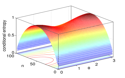
Figure 2: (Color online) Conditional entropy $\min_{\phi}S_{A|B}(\theta,\phi)$ [as shown in equation (20)] of Dicke state $|n\rangle_{N}$ as a function of $n$ and $\theta$ for fixed $N=100$. The minimum of $\min_{\phi}S_{A|B}(\theta,\phi)$ for fixed $n$ and $N$ is obtained at $\theta=\pi/2$.

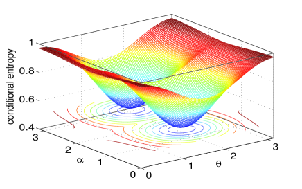
Figure 5: (Color online) Conditional entropy $\min_{\phi}S_{A|B}(\theta,\phi)$ [as shown in equation (20)] of the superposition of Dicke states $|\psi_{D}\rangle$ as a function of the angles $\alpha$ and $\theta$ for fixed $N=50$ and $n=30$. The minimum of $\min_{\phi}S_{A|B}(\theta,\phi)$ is obtained at $\theta=\pi/2$ for fixed $n$, $N$ and $\alpha$.

Many works have shown that the upper bound (22) is tight, i.e., $\min_{\theta,\phi}S_{A|B}\left(\theta,\phi\right)=\min\left\{S_{0},S_{1}\right\}$ [20, 27, 32]. However, for some two-qubit X-state, this upper bound is not necessary reachable, a counterexample is given in [58] (see the equation (18) therein). Fortunately, for the two-qubit density matricies which have been extracted from Dicke states and their superpositions, the matrix elements are shown in equation (28), our numerical results show that $\min_{\theta,\phi}S_{A|B}\left(\theta,\phi\right)=S_{1}$. That is, the minimum of $S_{A|B}\left(\theta,\phi\right)$ over $\theta$ is just obtained at the symmetric point $\theta=\frac{\pi}{2}$ (see exemplifications in figures 2 and 5). Therefore, we get the compact expression of the PQD for the two-qubit reduced density matrix (11) as

$$\mathcal{D}(\rho^{AB})=S(\rho^{B})-S(\rho^{AB})+S_{1},$$ (26)

where $S(\rho^{AB})$, $S(\rho^{B})$ and $S_{1}$ are given in equations (12), (15) and (24) respectively. In the following, we will apply equation (26) to study the pairwise quantum correlation of Dicke states and their superpositions.

Meanwhile, the PEoF for the reduced density matrix (11) is given by equation (8) with the concurrence expressed in [59],

$$C=\left\{\begin{array}[c]{cc}2(|u|-y),|u|\geq y;\\ 2(y-\sqrt{v_{+}v_{-}}),y\geq\sqrt{v_{+}v_{-}}.\end{array}\right.$$ (27)

4 Symmetric multi-qubit states

The state (11) can be obtained from the two-qubit reduced density matrix of Dicke states or their superposition states. In this case, the elements of the density matrix can be expressed in terms of the expectation values of the collective spin operators

$$v_{\pm}=\frac{N^{2}-2N+4\left\langle J_{z}^{2}\right\rangle\pm 4\left\langle J_{z}\right\rangle(N-1)}{4N(N-1)},~{}~{}y=\frac{N^{2}-4\left\langle J_{z}^{2}\right\rangle}{4N(N-1)},~{}~{}u=\frac{\left\langle J_{+}^{2}\right\rangle}{N(N-1)}.$$ (28)

where the collective spin operators are defined as $J_{\gamma}=\sum_{i=1}^{N}\frac{\sigma_{i\gamma}}{2}$ $\left(\gamma=x,y,z\right)$ with $N$ the total spin number and $\sigma_{i\gamma}$ the pauli operator on $i$-th site of spin. In the following, in terms of the PQD shown in equation (26), we would like to study the pairwise correlation of the X states (11) with the special elements shown in equation (28). In addition, the results will be compared with those obtained from PEoF, which is obtained by inserting equation (27) into equation (8).

4.1 Dicke state

A $N$-qubit Dicke state is defined as

$$\left|n\right\rangle_{N}=\left|\frac{N}{2},-\frac{N}{2}+n\right\rangle_{N},n=0,...,N,$$ (29)

and $\left|0\right\rangle_{N}=\left|\frac{N}{2},-\frac{N}{2}\right\rangle$ indicates that all spins are pointing down. $N$ is the total spin number, and $n$ is the excitation number of spins [60]. The expressions for the relevant spin expectation values can be easily obtained as [56],

$$\langle J_{z}\rangle=n-\frac{N}{2},~{}~{}\langle J_{z}^{2}\rangle=(n-\frac{N}{2})^{2},~{}~{}\langle J_{+}^{2}\rangle=0.$$ (30)

From equation (28), it is easy to see that the matrix elements of the reduced density matrix $\rho^{AB}$ are given by

$$v_{+}=\frac{n(n-1)}{N(N-1)},~{}~{}v_{-}=\frac{(N-n)(N-n-1)}{N(N-1)},~{}~{}y=\frac{n(N-n)}{N(N-1)},~{}~{}u=0.$$ (31)

In figure 2, we give a numerical check that, for any $N$ and $n$, the minimum of the conditional entropy $\min_{\phi}S_{A|B}(\theta,\phi)$ [as shown in equation (20)] are always obtained at $\theta=\pi/2$. The expression of PQD for Dicke states can be obtained by inserting equation (31) into equation (26).

The corresponding expression of PEoF is obtained by inserting into equation (27) and equation (8). The two expressions are a little lengthy, so we don’t explicitly write them down.

First, we fixed the spin number $N$ to see the behavior of PQD and PEoF for different excitation number $n$. For $n=0$ or $N$, the Dicke state becomes a product state, which has zero PQD and zero PEoF, i.e.,

$$\mathcal{D}(\rho_{\left|n\right\rangle_{N}}^{AB})=E_{F}(\rho_{\left|n\right\rangle_{N}}^{AB})=0.$$ (32)

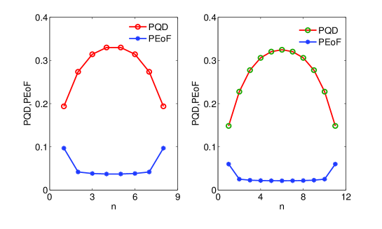
Figure 3: (Color online) PQD and PEoF of Dicke state $|n\rangle_{N}$ for different excitation number $n\in\left[1,N-1\right]$ with the fixed particle number $N=9$ (left) and $12$ (right).

In the following, we are interested in the cases that $n\in[1,N-1]$. As shown in figure 3, when $N$ is even, the PQD reaches to its maximum at $n=\frac{N}{2}$, and the Dicke state reads $\left|n\right\rangle_{N}=\left|\frac{N}{2}\right\rangle_{N}$, which has equal numbers of spins pointing up and down. When $N$ is odd, the PQD arrives its maximum at the point $n=\frac{N\pm 1}{2}$, where the Dicke state $\left|n\right\rangle_{N}=\left|\frac{N}{2}\pm\frac{1}{2}\right\rangle_{N}$ has the minimum different numbers of spins pointing up and down. However, no matter $N$ is even or odd, the maximum value of PEoF is obtained at the points $n=1$ or $N-1$, where the Dicke states have the maximum different numbers of spins pointing up and down, which are identical with the $W$ state as shown in the equation (33). The different behaviors of PQD and PEoF come from the different definitions of them, as illustrated in Sec. 2. Therefore, a state with maximum quantum correlation may not have maximum quantum entanglement.

Second, we discuss the behaviors of PQD and PEoF for different spin number $N$ with fixed excitation number $n$. For $n=1$, the Dicke state becomes a generic $W$ state

$$\left|1\right\rangle_{N}=\frac{1}{\sqrt{N}}(\left|11\cdots 10\right\rangle+\left|11\cdots 01\right\rangle+\cdots+\left|01\cdots 11\right\rangle),$$ (33)

and the PQD reduces to

$$\mathcal{D}(\rho^{AB}_{\left|1\right\rangle_{N}})=H\left(\frac{1}{N}\right)-H\left(\frac{2}{N}\right)+H\left(\frac{N+\sqrt{(N-2)^{2}+4}}{2N}\right).$$ (34)

On the other hand, the corresponding PEoF is given by

$$E_{F}(\rho^{AB}_{\left|1\right\rangle_{N}})=\max_{n\in[1,N-1]}E_{F}(\rho_{\left|n\right\rangle_{N}}^{AB})=H\left(\frac{N+\sqrt{N^{2}-4}}{2N}\right).$$ (35)

It is easy to check that

$$\mathcal{D}(\rho^{AB}_{\left|1\right\rangle_{N}})\geq E_{F}(\rho^{AB}_{\left|1\right\rangle_{N}}).$$ (36)

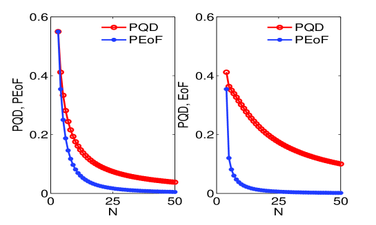
Figure 4: (Color online) PQD and PEoF of Dicke state $|n\rangle_{N}$ for different particle numbers $N\geq 3$ with fixed excitation $n=1$ (left) and $3$ (right).

For $n\geq 1$, the similar relation between the PQD and the PEoF are numerically shown in figure 4. Both of them decrease as the particle number $N$ increases, but the PQD reduces more slowly than PEoF. That is, for an arbitrary Dicke state, the general pairwise quantum correlation characterized by the PQD is more robust against the increasing of the total particle number of the Dicke ststes. This result is consistent with those obtained for the reduced two-qubit states under a decoherence environment [18, 19, 20].

4.2 Superposition of Dicke states

Then we consider a simple superposition of Dicke states as

$$\left|\psi_{D}\right\rangle=\cos\alpha\left|n\right\rangle_{N}+e^{i\delta}\sin\alpha\left|n+2\right\rangle_{N},$$ (37)

where $n=0,...,N-2$, the angle $\alpha\in[0,\pi)$ and the relative phase $\delta\in[0,2\pi)$. The expressions of the relevant spin expectations are

$$\left\langle J_{z}\right\rangle=\left(n-\frac{N}{2}\right)\cos^{2}\alpha+\left(n+2-\frac{N}{2}\right)\sin^{2}\alpha,$$

$$\left\langle J_{z}^{2}\right\rangle=\left(n-\frac{N}{2}\right)^{2}\cos^{2}\alpha+\left(n+2-\frac{N}{2}\right)^{2}\sin^{2}\alpha,$$

$$\left\langle J_{+}^{2}\right\rangle=\frac{1}{2}e^{i\delta}\sin 2\alpha\sqrt{\mu_{n}},$$ (38)

with $\mu_{n}=(n+1)(n+2)(N-n)(N-n-1)$.

For the state $\left|\psi_{D}\right\rangle$, the minimization of the conditional entropy $S_{A|B}\left(\theta,\phi\right)$ over the measurement phase $\phi$ is obtained at $\phi=\frac{1}{2}\delta$ or $\frac{1}{2}\delta+\pi$ according to the equation (3). Thus, the final expression of the PQD is independent of the superposition phase $\delta$ from the equation (21). In figure 4, we also numerically check that the conditional entropy $\min_{\phi}S_{A|B}(\theta,\phi)$ [as shown in equation (20)] of the state $\left|\psi_{D}\right\rangle$ arrives its minimum at $\theta=\frac{\pi}{2}$ for fixed $N$, $n$, and $\alpha$. Therefore, the analytical expression (26) for the superpositions of Dicke states is still valid.

There is a symmetry property of the PQD (or PEoF) for $\left|\psi_{D}\right\rangle$. From equation  (38), we observe that if we let $n\rightarrow N-n-2$ and $\alpha\rightarrow\frac{\pi}{2}+\alpha$, then $\left\langle J_{z}\right\rangle\rightarrow-\left\langle J_{z}\right\rangle$ and $\left\langle J_{+}^{2}\right\rangle\rightarrow-\left\langle J_{+}^{2}\right\rangle$, and furthermore $v_{+}\rightarrow v_{-}$ , $v_{-}\rightarrow v_{+}$ and $u\rightarrow-u$. Finally, two meaningful relations are obtained as

$$\mathcal{D}(N,n,\alpha,\delta)=\mathcal{D}\left(N,N-(n+2),\frac{\pi}{2}+\alpha,\phi\right),$$ (39)

and

$$E_{F}(N,n,\alpha,\delta)=E_{F}\left(N,N-(n+2),\frac{\pi}{2}+\alpha,\phi\right).$$ (40)

That is, both the PQD and PEoF are symmetrical about $n=N/2-1$ and $\alpha=-\pi/4$. These are useful properties for the following analysis.

Next we would like to discuss the relation between the PQD and PEoF for the state $\left|\psi_{D}\right\rangle$. First, when $N=2$ and $n=0$, the superposition of Dicke states becomes a two-qubit GHZ-like state,

$$\left|\psi_{D}\right\rangle=\cos\alpha\left|2\right\rangle+e^{i\delta}\sin\alpha\left|0\right\rangle.$$ (41)

This is a bipartite pure state so that the PQD equals PEoF, i.e.,

$$\mathcal{D}=E_{F}=H\left(\cos^{2}\alpha\right).$$ (42)

This is also the result for the case that $N=2$ and $n=1$ according to the symmetry properties  (39) and (40). In fact, for a general multi-qubit GHZ-like state with $N\geq{3}$

$$|\rm{GHZ}\rangle=\cos\alpha\left|N\right\rangle_{N}+e^{i\delta}\sin\alpha\left|0\right\rangle_{N},$$ (43)

there is no quantum correlation for the two-qubit reduced state, i.e.,

$$\mathcal{D}=E_{F}=0.$$ (44)

In summary, for a multi-qubit GHZ-like state, the PQD is always equal to the PEoF. Their values are always zero except for $N=2$.

Second, when $N=3$, it is interesting that, for any $n$, the state $\left|\psi_{D}\right\rangle$ has equal PQD and PEoF. In fact, for $N=3$ and $n=0$, the elements of the reduced density matrix are

$$v_{+}=y=\frac{\sin^{2}\alpha}{3},v_{-}=\cos^{2}\alpha,u=\frac{\sqrt{3}e^{i\delta}\sin 2\alpha}{6}.$$ (45)

And for $N=3$ and $n=1$, they are

$$v_{-}=y=\frac{\sin^{2}\alpha}{3},v_{+}=\cos^{2}\alpha,u=\frac{\sqrt{3}e^{i\delta}\sin 2\alpha}{6}.$$ (46)

Both of them satisfy the relation that

$$v_{+}=y,~{}~{}~{}~{}v_{+}v_{-}=|u|^{2}.$$ (47)

This ensures the joint entropy $S\left(\rho_{|\psi\rangle_{D}}^{AB}\right)$ equals the reduced entropy $S\left(\rho_{|\psi\rangle_{D}}^{A}\right)$, i.e.,

$$S\left(\rho_{|\psi\rangle_{D}}^{AB}\right)=S\left(\rho_{|\psi\rangle_{D}}^{A}\right).$$ (48)

Therefore, the PQD is

$$\mathcal{D}=\min_{\theta,\phi}S_{A|B}(\theta,\phi)=S_{1}=H\left(\frac{1+\kappa_{1}}{2}\right),$$ (49)

with

$$\kappa_{1}=\sqrt{(v_{+}-v_{-})^{2}+4(y+|u|)^{2}}.$$ (50)

Meanwhile, from equation  (47), the corresponding concurrence is given by

$$C^{2}=4(y-|u|)^{2}.$$ (51)

Obviously,

$$\kappa_{1}=\sqrt{1-C^{2}}.$$ (52)

Thus, PQD is equal to PEoF, i.e.,

$$\mathcal{D}=E_{F}.$$ (53)

Combining the symmetry properties (39) and (40), this equivalence can be extended to any $n$ for $N=3$. This indicates that for certain kinds of mixed state, quantum entanglement may also represents the whole quantum correlation.

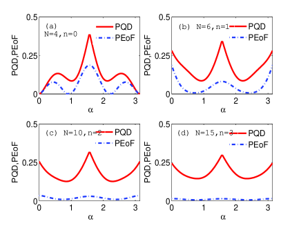
Figure 6: (Color online) PQD and PEoF for superposition of Dicke state $|\psi_{D}\rangle$ as the function of $\alpha$ for different $N\geq{4}$ and $n$.

Both of the above two cases with $N=2$ and $N=3$ show that PQDs are equal to PEoFs for pure and some special mixed two-qubit states. However, when $N\geq 4$, the equivalence does not always hold, as shown in figure  6. It seems that the PQD is always greater than or equal to PEoF. This is similar to the case of Dicke states. In addition, the results are a little more complex than that of Dicke state. Every possible cases exists. The state with maximum (minimum) PEoF may have (or not have) the maximum (minimum) PQD as shown in figure  6 (a) and (b) for small particle number $N$. While for large $N$, as shown in figure 6 (c) and (d), the state with maximum (minimum) PEoF approaches to the one with the maximum (minimum) PQD.

4.3 Spin coherent states

Finally, we consider two more complex superpositions of Dicke states, i.e., the superpositions of the form $\sum_{n}C_{n}\left|n\right\rangle_{N}$ with the excitation numbers $n$ even and odd respectively. They can be given by SCSs [49, 61, 62]

$$\left|\eta\right\rangle_{\pm}=\frac{1}{\sqrt{2(1\pm\gamma^{N})}}(\left|\eta\right\rangle\pm\left|-\eta\right\rangle),$$ (54)

with $\gamma=(1-\eta^{2})/(1+\eta^{2})$. The $``\pm``$ corresponds to the so called even SCSs (ESCSs) and odd SCSs (OSCSs), respectively. A SCS is obtained by a rotation of the Dicke state $\left|0\right\rangle_{N},$

$$\left|\eta\right\rangle=(1+\eta^{2})^{-N/2}\exp{(J_{+}\eta)}|0\rangle_{N}=(1+\eta^{2})^{-N/2}\sum_{n=0}^{N}\left(\begin{array}[c]{c}N\\ n\end{array}\right)^{1/2}\eta^{n}\left|n\right\rangle_{N},$$ (55)

where the parameter $\eta\in[0,1]$. The expectations for the ESCSs and OSCSs are

$$\left\langle J_{z}\right\rangle_{\pm}=\frac{-N}{2}\frac{\gamma\pm\gamma^{N-1}}{1\pm\gamma^{N}},$$

$$\left\langle J_{z}^{2}\right\rangle_{\pm}=\frac{N^{2}}{4}\pm\frac{N(N-1)\eta^{2}\upsilon_{\eta}^{\mp}}{1\pm\gamma^{N}},$$

$$\left\langle J_{+}^{2}\right\rangle_{\pm}=\pm\frac{N(N-1)\eta^{2}\upsilon_{\eta}^{\pm}}{1\pm\gamma^{N}},$$ (56)

with $\upsilon_{\eta}^{\pm}=\gamma^{N}(1-\eta^{2})^{-2}\pm(1+\eta^{2})^{-2}$.

Similar to the above two cases shown in Secs. 4.1 and 4.2, we also numerically check that the analytical expression (26) of PQD can be reliably accepted. Here the expression of PQD is so lengthy that we only numerically show its behaviors for different parameters, as displayed in figure 7. We see that, when $\eta$ is small, the QD of OSCSs is always greater than that of ESCSs for fixed particle number $N\geq 3$. However, when $\eta$ becomes large and approaches $1$, they become gradually equal to each other. Especially, when $N\gg 1$, they coincide with each other even for small $\eta$. All these results can be explained analytically from the three special cases in the following.

When $\eta\rightarrow 0$, the PQD of the OSCS is different from that of the ESCS . The OSCS reduces to the Dicke state $\left|\eta=0\right\rangle_{-}=\left|1\right\rangle_{N}$ (the $W$ state shown in equation (33)), whose PQD is nonzero as shown in equation (34). Meanwhile, the ESCS reduces to product state $\left|\eta=0\right\rangle_{+}=\left|0\right\rangle_{N}$, then $\mathcal{D}=0$, as shown in figure 7.

However, when $\eta\rightarrow 1$, the PQDs of OSCSs and ESCSs coincide with each other. In this case, both of the OSCSs and ESCSs reduces to GHZ states in the $x$ direction [62],

$$\left|\eta=1\right\rangle_{\pm}=\frac{1}{\sqrt{2}}((\left|N\right\rangle_{N})_{x}\pm(\left|0\right\rangle_{N})_{x}).$$ (57)

If $N\geq 3$, the reduced density matrix of the OSCSs and ESCSs are diagonalized

$$\rho^{AB}|_{\eta=1}=\frac{1}{2}\left|00\right\rangle\left\langle 00\right|+\frac{1}{2}\left|11\right\rangle\left\langle 11\right|,$$ (58)

and we have $\mathcal{D}=0$.

Finally, when $N\gg 1$, for both the OSCSs and ESCSs, the reduced density matrices are almost independent of $N$,

$$\rho^{AB}|_{N\gg 1}=\frac{1}{(1+\eta^{2})^{2}}\left(\begin{array}[c]{cccc}1&0&0&\eta^{2}\\ 0&\eta^{2}&\eta^{2}&0\\ 0&\eta^{2}&\eta^{2}&0\\ \eta^{2}&0&0&\eta^{4}\end{array}\right),$$ (59)

and PQD can be given by

$$\mathcal{D}(\rho^{AB}|_{N\gg 1})=H\left(\frac{1}{1+\eta^{2}}\right)-H\left(\frac{2\eta^{2}}{(1+\eta^{2})^{2}}\right)+H\left(\frac{(1+\eta^{2})^{2}+\sqrt{1+14\eta^{4}+\eta^{8}}}{(1+\eta^{2})^{2}}\right).$$

Then PQD will also become independent of $N$. As a result, PQDs of OSCSs and ESCSs become close to each other even for small $\eta$, as shown in figure  7 (d). In particular, we obtain $E_{F}(\rho^{AB}|_{N\gg 1})=0$. This implies that QD is a more general measure of quantum correlation than quantum entanglement. For a set of quantum separable states, they do have quantum correlations.

In figure 8, we display the relation of maximum PQDs between the OSCSs and ESCSs over the parameter scale $\eta\in\left[0,1\right]$. It shows that the maximum PQD of OSCSs is always greater than or equal to that of ESCSs for fixed particle number $N$. When $N\gg 1$, their maximum values attain a constant, which can also be seen from figure  7.

5 Conclusion

In terms of PQD, we have investigated the pairwise quantum correlations in Dicke states and their superpositions in terms of its two-qubit density matrix, whose elements may be complex. A general expression for PQD is derived according to the numerical proof. For the Dicke states, our analytical and numerical results show that the PQD is always greater than or equal to the PEoF. This further proves that QD is a more general measure of quantum correlation than quantum entanglement. For the superpositions of Dicke states, it is interesting that the QD is always equal to EoF when $N=2$ (GHZ-like states) and $N=3$ (W states), which indicates that for some kinds of mixed states, quantum correlation can also be fully described by quantum entanglement. For OSCSs and ESCSs, the former always show more quantum correlations than the latter. In addition, the PQD is generally more robust against the enlarging of the particle number of the multi-qubit states, which implies that PQD has an advantage over pairwise entanglement in characterizing the quantum correlation in the multi-qubit states. To some extent, the pairwise quantum correlations of the reduced states may reflect the multi-qubit quantum correlations of the global states.

References

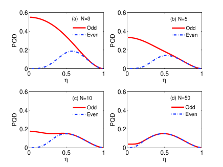
Figure 7: (Color online) PQD for odd and even SCSs along with the parameter $\eta\in\left[0,1\right]$ for different spin numbers $N$.

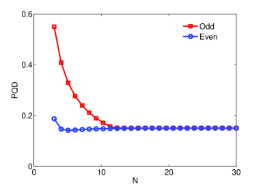
Figure 8: (Color online) Maximum PQD of the ESCSs and OSCSs over the parameter scale $\eta\in\left[0,1\right]$ for different $N\geq 3$.

References

- [1] Nielsen M A and Chuang I L, Quantum Computation and Quantum information (Cambridge University Press, Cambridge, 2000)
- [2] Vedral V 2002 Rev. Mod. Phys. 74 197
- [3] Plenio M B and Virmani S 2007 Quant. Inf. Comp. 7 1
- [4] Horodecki R et al2009 Rev. Mod. Phys. 81 865
- [5] Wootters W K 1998 Phys. Rev. Lett. 80 2245 ; Wootters W K 2001 Quant. Inf. Comp. 1 27
- [6] Groisman B et al2005 Phys. Rev. A 72 032317
- [7] Horodecki M et al2005 Phys. Rev. A 71, 062307
- [8] Bennett C H et al1999 Phys. Rev. A 59 1070
- [9] Lanyon B P et al2008 Phys. Rev. Lett. 101 200501
- [10] Datta A et al2005 Phys. Rev. A 72 042316; Datta A and Vidal G 2007 Phys. Rev. A 75 042310; Datta A et al2008 Phys. Rev. Lett. 100 050502;
- [11] Ollivier H and Zurek W H 2002 Phys. Rev. Lett. 88 017901
- [12] Zurek W H 2000 Ann. Phys. 9 855; Zurek W H 2003 Phys. Rev. A 67 012320
- [13] Henderson L and Vedral V 2001 J. Phys. A 34 6899
- [14] Vedral V 2003 Phys. Rev. Lett. 90 050401
- [15] Ferraro A et al2010 Phys. Rev. A 81 052318
- [16] Cavalcanti D et al2011 Phys. Rev. A 83 032324
- [17] Madhok V and Datta A 2011 Phys. Rev. A 83 032323
- [18] Werlang T et al2009 Phys. Rev. A 80 024103
- [19] Maziero J et al2010 Phys. Rev. A 81 022116
- [20] Fanchini F F et al2010 Phys. Rev. A 81 052107
- [21] Piani M et alPhys.Rev. Lett. 102 250503
- [22] Dillenschneider R 2008 Phys. Rev. B 78 224413
- [23] Sarandy M S 2009 Phys. Rev. A 80 022108
- [24] Chen Y and Li S 2010 Phys. Rev. A 81 032120
- [25] Werlang T and Rigolin G 2010 Phys. Rev. A 81 044101
- [26] Shabani A and Lidar D A 2009 Phys. Rev. Lett. 102 100402
- [27] Luo S 2008 Phys. Rev. A 77 042303; Luo S 2008 Phys. Rev. A 77 022301
- [28] Maziero J et al2010 Phys. Rev. A 82 012106
- [29] Datta A and Gharibian S 2009 Phys. Rev. A 79 042325 ; Datta A 2009 Phys. Rev. A 80 052304
- [30] Wu S et al2009 Phys. Rev. A 80 032319
- [31] Csar A Rodríguez-Rosario et al2008 J. Phys. A: Math. Theor. 41 205301
- [32] Ali M et al2010 Phys. Rev. A 81 042105
- [33] Brodutch A and Terno D R 2010 Phys. Rev. A 81 062103
- [34] SaiToh A et al2008 Phys. Rev. A 77 052101
- [35] Kaszlikowski D et al2007 Phys. Rev. Lett. 101 070502
- [36] Modi K et al2010 Phys. Rev. Lett. 104 080501
- [37] Fanchini F Fet al2011 Phys. Rev. A 84, 012313
- [38] Chen Y X and Yin Z 2010 Commun. Theor. Phys 54 60
- [39] Hao X et al2011 Commun. Theor. Phys 55 41
- [40] J. Xu et al2010 Nat.Commun. 1, 7
- [41] J. Xu et al2010 Phys. Rev. A 82, 042328
- [42] Auccaise R et al2011 Phys. Rev. Lett. 107 140403
- [43] Mølmer K, 1999, Eur. Phys. J. D, 5, 301; Kuzmich A, Bigelow N P, and Mandel L, 1998, Europhys.Lett., 42, 481
- [44] Lemr K and Fiurášek J, 2009, Phys. Rev. A , 79, 043808
- [45] Matthews J C F, Politi A, Stefanov A, and O Brien J L, 2009, arXiv:0911.1257
- [46] Zeilinger A, Horne M A, and Greenberger D M, 1997, NASA Conf. Publ. No. 3135
- [47] Dür W, Vidal G, and Cirac J I, 2000, Phys. Rev. A 62, 062314
- [48] Greenberger D M, Horne M A, and Zeilinger A, 1995, Phys. Rev. Lett. 75, 2064
- [49] Radcliffe J M, 1971, J. Phys. A 4, 313
- [50] Kitagawa M and Ueda M, 1993, Phys. Rev. A 47, 5138
- [51] Agrawal P and Pati A, 2006, Phy. Rev. A 74, 062320
- [52] Tóth G, 2007, J. Opt. Soc. Am. B 24, 275
- [53] Linden N, Popescu S and Wootters W K, 2002, Phys. Rev. Lett. , 89, 207901
- [54] Walck S N and Lyons D W, 2008, Phys. Rev. Lett., 100, 050501; Walck S N and Lyons D W, 2009, Phys. Rev. A 79, 032326
- [55] Diosi L, 2004, Phys. Rev. A, 70, 010302; Jones N S and Linden N, 2005, Phys. Rev. A, 71, 012324; Zhou D L, 2008, Phys. Rev. Lett., 101, 180505
- [56] Wang X G and Mølmer K 2002 Eur. Phys. J. D. 18 385
- [57] T. M. Cover and J. A. Thomas, Elements of Information Theory (Wiley Interscience, New York, 2006).
- [58] Lu X M et al, 2011, Phys. Rev. A 83, 012327
- [59] Vidal J 2006 Phys. Rev. A 73 062318
- [60] Dicke R H 1954 Phys. Rev. 93 99
- [61] Gerry C C and Grobe B 1998 Phys. Rev. A 57 2247
- [62] Arecchi F T et al1972 Phys.Rev. A 6 2211