Relativistic Two-Body Coulomb-Breit Hamiltonian in an External Weak Gravitational Field

Abstract

A construction of the Coulomb-Breit Hamiltonian for a pair of fermions, considered as a quantum two-body system, immersed in an arbitrary background gravitational field described by Einstein’s General Relativity is presented. Working with Fermi normal coordinates for a freely falling observer in a spacetime region where there are no background sources and ignoring the gravitational back-reaction of the system, the effective Coulomb-Breit Hamiltonian is obtained starting from the S-matrix element corresponding to the one-photon exchange between the charged fermionic currents. The contributions due to retardation are considered up to order $(v/c)^{2}$ and they are subsequently written as effective operators in the relativistic quantum mechanical Hilbert space of the system. The final Hamiltonian includes effects linear in the curvature and up to order $(v/c)^{2}$.

1 Introduction

The connection between Einstein’s General Relativity (GR), the dynamical theory of space-time, and Quantum Mechanics (QM) has a long history in physics and more than ever is nowadays a subject of intense research, both from theoretical and experimental perspectives, mainly in connection with possible deviations from GR and/or QM. Until now, experiments have already confirmed that inertia and Newtonian gravity affect quantum particles, mainly electrons and neutrons, in ways that are fully consistent with GR down to distances of the order of ${10^{-8}}\,\rm{cm}$. Gravitational-inertial fields leave their mark on particle wave functions in a variety of ways; particularly, they induce quantum phases that have been measured in some of the most renowned experiments on this topic [1, 2, 3, 4, 5, 6]. Recently, the purpose of tests of gravity has been mainly focused in determining the validity of the equivalence principle at the level of atoms, molecules, quasi-particles and antimatter. This translates into a need for higher precision tests of GR, and atomic physics together with quantum optics offer some of the most accurate results and promising scenarios.

Most of the experimental tests of GR within the quantum realm arise from predictions on fully covariant wave equations where inertia and gravity appear as external classical fields, providing very valuable information on how Einstein’s views carry through into the quantum world. However, many of the initially proposed and tested effects considered mainly one-particle systems. This approach leaves aside the possibility of using the internal quantum structure of atoms or molecules as additional parameters. Nevertheless, this situation is drastically changing recently due to the fast development of matter wave interferometry [7, 8, 9].

Broadly speaking, previous work related to the description of atoms in a background gravitational field can be divided in three main branches, though with much interrelation among them: (i) the study of gravitational modifications to atomic spectra of mainly hydrogen-like atoms, which were considered as a quantum reduced mass revolving around some force center [10, 11, 12, 13, 14, 15, 16, 17, 18, 19, 20, 21]. A two-body description of the atom can be found in Refs. [22, 23, 24]. (ii) Restricted proofs of the equivalence principle for test bodies made of classical electromagnetically interacting particles, within the PPN framework or within the $TH\epsilon\mu$ formalism for static spherically symmetric spacetimes [25, 26, 27, 28]. The formulation of a quantum equivalence principle has been studied in Refs. [29, 30]. (iii) Tests and studies of the gravitational red shift, where atomic clocks were described as quantum mechanical systems within the $TH\epsilon\mu$ or PPN formalisms [31, 32, 33, 34, 35, 36, 37].

In this letter we consider the effect of a classical background gravitational field, described by GR, upon matter at the atomic level, where the use of QM becomes mandatory. We extend previous work in the following aspects: (i) We will consider the case of hydrogen-like atoms described as two-body systems in the way first discussed in Ref. [23]. The inclusion of the position of the atom as a new degree of freedom may provide additional couplings to probe the effects of gravity upon quantum objects in the region where tidal forces become important. (ii) The background gravitational field has no particular spatial symmetry. (iii) Following the steps of Ref. [38], a quantum mechanical relativistic two-body effective potential in the background gravitational field is produced, which takes into account retardation effects arising from the one-photon exchange between the currents. This constitutes the gravitational generalization of the relativistic Coulomb-Breit potential [39].

Most of the general assumptions underlying this work are similar to those of Refs.[10, 13, 15, 23, 25, 26]: (i) The external gravitational field is well described by GR, so that it satisfies Einstein’s field equations. Additionally, we ignore back-reaction effects. (ii) All the interacting particles are influenced by the background gravitational field at the quantum level. (iii) There exists an ideal freely falling observer in a region outside the sources of the background gravitational field. This observer determines that, in his coordinate patch, the metric of the spacetime has the form

$$g_{\alpha\beta}=\eta_{\alpha\beta}+{\cal Q}_{\alpha b\beta c}x^{b}x^{c}\equiv\eta_{\alpha\beta}+h_{\alpha\beta}\left(x^{0}\right),$$ (1)

where

$${\cal Q}_{0a0b}=-\breve{R}_{0a0b}\left(x^{0}\right),\,\,{\cal Q}_{0abc}=-\frac{2}{3}\breve{R}_{0abc}\left(x^{0}\right),\,\,{\cal Q}_{abcd}=-\frac{1}{3}\breve{R}_{abcd}\left(x^{0}\right).$$ (2)

Here $x^{a}$ are three spatial coordinates, $x^{0}$ is the proper time of the observer and $\breve{R}_{\alpha\beta\gamma\delta}$ is the projection of the background Riemann tensor on the orthonormal tetrad carried by him, which in general depends on the proper time due to the motion of the observer. The weakness of the gravitational interaction induces very small corrections upon the observables, so that in our final results we preserve only quantities up to first order in $\breve{R}_{\alpha\beta\gamma\delta}$. The metric (1) is that of a freely falling observer using Fermi normal coordinates, which are appropriate to describe local experiments performed by inertial observers [40]. (iv) The spatial extension and the time duration of events related to observations in the quantum system are very small compared with the characteristic lengths and times of appreciable changes in the observer’s Riemann tensor [15]. This allows well defined energy levels and the use of time-independent perturbation theory. Within this adiabatic approximation it is possible to ignore the $x^{0}$ dependence of the metric and of all the objects constructed from it: the time coordinate becomes just a fixed but arbitrary parameter [26]. (v) Conditions (i) and (iii) imply that the observer determines that his Ricci tensor ${{\breve{R}}^{\alpha}{}_{\beta}}$ is equal to zero. We also assume that during the measurements performed by the observer there are no particle creation effects due to the gravitational field.

The coupled equations that describe the electromagnetic interaction between spin $1/2$ fermions in a background gravitational field, outside the gravitational sources, are

$$ic\hbar\gamma^{\mu}D_{\mu}\psi-mc^{2}\psi=q\gamma^{\mu}\psi A_{\mu},\qquad D^{\mu}D_{\mu}A^{\nu}=q\bar{\psi}\gamma^{\nu}\psi\equiv{J}^{\nu},$$ (3)

where we have chosen the Lorentz gauge $D_{\mu}A^{\mu}=0$. Here $D_{\mu}=\partial_{\mu}-\frac{i}{2}\omega^{BD}{}_{\mu}J_{BD}$ is the covariant derivative written in general terms, $\omega^{\bar{\alpha}}{}_{{\bar{\beta}}\mu}=e^{\bar{\alpha}}{}_{\delta}\left(D_{\mu}e_{\bar{\beta}}{}^{\delta}\right)$ is the spin connection, and $J_{BD}$ are the Lorentz group generators in the corresponding representation for each field.

2 The photon propagator

The fundamental quantity required to construct an effective relativistic Hamiltonian describing the electromagnetic interaction between two charges is the curved space Feynman Green function $G^{\mu}{}_{\nu^{\prime}}(x^{\prime},x)$ for the photon [41]. We consider its Hadamard representation because it is valid in all spacetimes [43]. The differential equation for the electromagnetic Feynman Green function is

$$\square\,G^{\alpha}{}_{\beta}(x,x^{\prime})=-\kappa^{\alpha}{}_{\beta}\left(x,x^{\prime}\right)\delta_{4}\left(x,x^{\prime}\right),$$ (4)

where $\square\equiv g^{\mu\nu}\nabla_{\mu}\nabla_{\nu}$, $\,\kappa^{\alpha}{}_{\beta}$ is the parallel propagator bitensor between $x^{\prime}$ and $x$, and $\delta_{4}\left(x,x^{\prime}\right)$ is the invariant Dirac delta distribution for our observer. The solution to (4), that vanishes at infinity for arbitrary time, is

$$G_{\alpha\beta}(x,x^{\prime})=\frac{1}{\left(2\pi\right)^{2}}\left(\frac{\kappa_{\alpha\beta}(x,x^{\prime})}{\sigma(x,x^{\prime})+i\epsilon}\right).$$ (5)

The expressions for the parallel propagator $\kappa^{\alpha}{}_{\beta}\left(x,x^{\prime}\right)\equiv\,e_{{\bar{\gamma}}}{}^{\alpha}\left(x\right)e^{{\bar{\gamma}}}{}_{\beta}\left(x^{\prime}\right)$ are

$$\kappa_{00} \circeq\eta_{00}+\frac{1}{2}\left[h_{00}\left(x\right)+h_{00}\left(x^{\prime}\right)\right],\qquad\kappa_{0a}\circeq\frac{1}{4}\left[3h_{0a}\left(x\right)+h_{0a}\left(x^{\prime}\right)\right],$$ (6)

$$\kappa_{a0} \circeq\frac{1}{4}\left[h_{0a}\left(x\right)+3h_{0a}\left(x^{\prime}\right)\right],\qquad\kappa_{ab}\circeq\eta_{ab}+\frac{1}{2}\left[h_{ab}\left(x\right)+h_{ab}\left(x^{\prime}\right)\right].$$ (7)

Here $\sigma(x,x^{\prime})$ is the Synge world function, given by

$$\sigma\left(x,x^{\prime}\right)\circeq\frac{1}{2}\eta_{\mu\nu}\left(x-x^{\prime}\right)^{\mu}\left(x-x^{\prime}\right)^{\nu}+\frac{1}{2}{\cal Q}_{\mu a\nu b}{\cal A}^{ab}\left(x-x^{\prime}\right)^{\mu}\left(x-x^{\prime}\right)^{\nu}.$$ (8)

with

$${\cal A}^{ab}\equiv\left[\frac{1}{2}\left(x^{\prime a}x^{b}+x^{a}x^{\prime b}\right)+\frac{1}{3}\left(x-x^{\prime}\right)^{a}\left(x-x^{\prime}\right)^{b}\right].$$ (9)

Note that expression (5) contains terms of higher order than first in the curvature, arising from the denominator $\sigma+i\epsilon$. We will keep the complete singular structure of the Green function because, in the following calculations, we will require expressions for the corresponding poles up to first order in $h_{\mu\nu}$. Let us remark that $\sigma(x,x^{\prime})=\sigma({\mathbf{x},\mathbf{x^{\prime}},x^{0}-x^{\prime 0}})$.

3 The one-photon interaction

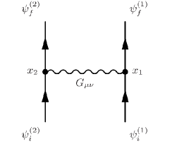
Figure 1: The one-photon exchange diagram leading to the effective interaction potential. Fermions and photons include the effects of the gravitational background.

In order to incorporate gravitational corrections into the electromagnetic interaction between two charged particles, we will use the S-Matrix method [41] as described in Ref.[38], but generalized to a slightly curved space [42]. We need to evaluate the S-matrix element corresponding to the exchange of one photon between the two fermionic currents located at $x_{2}$ and $x_{1}$, shown in Fig. (1), which is given by

$$S_{fi}^{\ \left(1\right)}=\frac{1}{c\hbar}\int J^{\mu\left(2\right)}_{fi}\left(x_{2}\right)G_{\mu\nu}\left(x_{2},x_{1}\right)J^{\nu\left(1\right)}_{fi}\left(x_{1}\right)\,d^{4}V_{2}\,d^{4}V_{1},$$ (10)

where $G_{\mu\nu}\left(x_{2},x_{1}\right)$ is the electromagnetic Feynman Green function (5) and $d^{4}V\equiv\sqrt{-g\left(x\right)}\ d^{4}x$ is the invariant volume element at point $x$. The transition current for each charge $q_{n}$ has the form given in Eq. (3). As a consequence of the adiabatic approximation, the Dirac fermions which describe the charged particles can be represented by spinors with a definite positive frequency, in the coordinate patch of our observer. We can write the spinor field as

$$\psi\left(y\right)=e^{-ik^{0}y^{0}}\Psi\left({\mathbf{y}}\right)\quad{\rm with}\quad k^{0}>0,$$ (11)

which satisfies the generalized Dirac equation given in (3). The explicit form for each current is

$$J^{\mu(n)}_{fi}(y)=\left[q_{n}\left(\Psi_{f}^{(n)}(\mathbf{y})\right)^{T*}\gamma^{\bar{0}}_{\left(n\right)}\gamma^{\mu}_{\left(n\right)}\left(\mathbf{y}\right)\Psi_{i}^{\left(n\right)}({\mathbf{y}})\right]e^{i\Delta_{fi}^{\left(n\right)}y^{0}},$$ (12)

where we have defined $\Delta_{fi}^{\left(n\right)}\equiv k^{0}{}_{f}^{\left(n\right)}-k^{0}{}_{i}^{\left(n\right)}$. Let us construct the two-particle states $\Phi_{i,f}\left(\mathbf{1},\mathbf{2}\right)$ as the usual direct product of the spinorial wave function $\Psi^{\left(n\right)}({\mathbf{x}})$ of each particle. We can then rewrite $S_{fi}^{\ \left(1\right)}$ as a matrix element of an operator ${\cal W}^{\left(\mathbf{1},\mathbf{2}\right)}$ between the initial and final two-particle states : $\Phi_{i}\left(\mathbf{2},\mathbf{1}\right)=\Psi^{(2)}_{i}(\mathbf{x}_{2})\otimes\Psi^{(2)}_{1}(\mathbf{x}_{1})$ and $\Phi_{f}\left(\mathbf{2},\mathbf{1}\right)=\Psi^{(2)}_{f}(\mathbf{x}_{2})\otimes\Psi^{(1)}_{f}(\mathbf{x}_{1})$, respectively, in such a way that

$$S_{fi}=\int\left(\Phi_{f}\right)^{T\ast}\left(\gamma_{(2)}^{\bar{0}}\gamma_{(2)}^{0}\right)\left(\gamma_{(1)}^{\bar{0}}\gamma_{(1)}^{0}\right){\cal W}^{\left(\mathbf{1},\mathbf{2}\right)}\,\Phi_{i}\,d^{4}V_{2}\,d^{4}V_{1}\equiv i\delta(\Omega)\,\langle\Phi_{f}|{\hat{\cal W}}_{e}|\Phi_{i}\rangle,$$ (13)

where $\Omega\equiv\Delta_{fi}^{\left(2\right)}+\Delta_{fi}^{\left(1\right)}$ and $\delta(\Omega)$ leads to energy conservation. Substituting (12) in (10) and with help of (13) we identify the operator

$${\cal W}^{\left(\mathbf{2},\mathbf{1}\right)}=\alpha_{e}\,\frac{\gamma^{0}_{\left(2\right)}\gamma^{\bar{\mu}}_{\left(2\right)}}{g^{00}\left({\mathbf{x}_{2}}\right)}\,\,{\cal G}_{{\bar{\mu}}{\bar{\nu}}}\left(\mathbf{2},\mathbf{1}\right)\frac{\gamma^{0}_{\left(1\right)}\gamma^{\bar{\nu}}_{\left(1\right)}}{g^{00}\left({\mathbf{x}_{1}}\right)},\qquad\alpha_{e}=-\left(\frac{q_{1}q_{2}}{\hbar c}\right),$$ (14)

where

$${\cal G}_{{\bar{\mu}}{\bar{\nu}}}({\mathbf{x}_{2}},{\mathbf{x}_{1}})=\frac{\eta_{{\bar{\mu}}{\bar{\nu}}}}{\left(2\pi\right)^{2}}\int\int\frac{e^{i\left(\Delta_{fi}^{\left(2\right)}x_{2}^{0}+\Delta_{fi}^{\left(1\right)}x_{1}^{0}\right)}}{\sigma\left(x_{2},x_{1}\right)+i\epsilon}dx_{2}^{0}dx_{1}^{0}\equiv\eta_{{\bar{\mu}}{\bar{\nu}}}\,\,I\left(\mathbf{2},\mathbf{1}\right).$$ (15)

From expression (14) for ${\cal W}^{\left(\mathbf{2},\mathbf{1}\right)}$ we will obtain the effective interaction operator, after evaluating the integrals in (15) and after choosing an ordering prescription to complete the construction. To first order in the curvature, the poles of the Synge function are slightly displaced along the real line with respect to those of the flat expression. Because of this, we can take in (15) the same integration contour used in the Minkoswki spacetime calculation, but inserting the modified poles. The result of the contour integration is

$$I\left(\mathbf{2},\mathbf{1}\right)=-i\delta\left(\Omega\right)\frac{e^{iw\frac{b_{0}}{\left(1-a_{00}\right)}}}{\left|\rho\right|\left(1-a_{00}\right)}\left[\theta\left(w\right)e^{iw\left|\rho\right|}+\theta\left(-w\right)e^{-iw\left|\rho\right|}\right],$$ (16)

where

$$w\equiv\Delta_{fi}^{\left(2\right)}-\Delta_{fi}^{\left(1\right)},\quad\quad\left|\rho\right|\circeq r\left[1+\frac{1}{2}\left(a_{00}+\frac{\xi_{h}}{r^{2}}\right)\right].$$ (17)

We have introduced the additional notation

$$\qquad\qquad r^{2}=\delta_{ab}\left(x_{2}-x_{1}\right)^{a}\left(x_{2}-x_{1}\right)^{b},\quad a_{00}={\cal Q}_{0a0b}{\cal A}^{ab},$$ (18)

$$b_{0}={\cal Q}_{0acb}{\cal A}^{ab}\left(x_{2}-x_{1}\right)^{c},\quad\xi_{h}={\cal Q}_{cadb}{\cal A}^{ab}\left(x_{2}-x_{1}\right)^{c}\left(x_{2}-x_{1}\right)^{d}.$$ (19)

Here ${\cal A}^{ab}$ is obtained from Eq. (9) by making the replacements $x^{\prime}\rightarrow x_{1},\,x\rightarrow x_{2}$. The study of the symmetry properties under the exchange ${\mathbf{1}}\leftrightarrow\mathbf{2}$ in Eqs. (13) and (14) leads to the property $I\left(\mathbf{2},\mathbf{1}\right)=I\left(\mathbf{1},\mathbf{2}\right)$, which can be directly verified in expression (16). Next we expand both exponentials up to order $w^{2}$ obtaining

$${\cal G}_{{{\bar{\mu}}}{{\bar{\nu}}}}=-i\delta\left(\Omega\right)\eta_{{{\bar{\mu}}}{{\bar{\nu}}}}\left\{\frac{1}{r}\left[1+\frac{1}{2}\left(a_{00}-\frac{\xi_{h}}{r^{2}}\right)\right]+i\left(\frac{w\,b_{0}}{2r}\right)\right.$$

$$\qquad\qquad\left.-\frac{r}{2}\left(\frac{w^{2}}{4}\right)\left(1+\frac{1}{2}\left(3a_{00}+\frac{\xi_{h}}{r^{2}}\right)\right)\right\}.$$ (20)

The above expression still contains terms of order higher than first in the curvature because $w\circeq w_{0}+w_{h}$. The final reduction to the desired order will be obtained after we rewrite the powers of $w$ as functions of the one-particle Hamiltonian in the presence of a gravitational background

$$\qquad\hat{\cal{H}}\circeq-\frac{c}{4}\gamma^{\bar{a}}\gamma^{\bar{b}}h_{0a}\hat{p}_{b}+c\gamma^{\bar{0}}\gamma^{\bar{a}}\left(-\hat{p}_{a}+\frac{1}{2}h^{c}{}_{a}\hat{p}_{c}+\frac{1}{2}h_{00}\hat{p}_{a}\right)$$

$$-i\hbar c\gamma^{\bar{0}}\gamma^{\bar{\mu}}\Gamma_{\mu}\left(x\right)-\frac{3c}{4}h^{a}{}_{0}\hat{p}_{a}+imc^{2}\left(1-\frac{1}{2}h_{00}\right)\gamma^{\bar{0}}+\frac{i}{4}mc^{2}h_{0a}\gamma^{\bar{a}},$$ (21)

which is hermitian in the curved inner product

$$\langle\phi,\psi\rangle=-\int\phi^{T\ast}\,\gamma^{\bar{0}}\gamma^{0}\,\psi\,\sqrt{-g}\,\,d^{3}x.$$ (22)

Let us recall that in Eq. (3) we have expanded all curved quantities up to first order in the curvature, which explains the contraction between tetrad and coordinate indexes that appears. This feature will frequently repeat itself in what follows.

4 The effective relativistic interaction

The effective interaction operator $\hat{{\cal W}}_{e}$ is constructed in such a way that the $w$-dependent contributions in (3) arise as a consequence of taking the matrix elements of $\hat{{\cal W}}_{e}$ indicated in the right hand side of Eq. (13). The operator $\hat{{\cal W}}_{e}$ will be a matrix operator acting on the quantum-mechanical Hilbert space of the system. To perform such construction we use the identification ${\hat{p}}_{a}=-i\hbar\partial_{a}$ in (3), together with the eigenvalue equation for each spinor and Eq. (3). We start by substituting (3) in (13) in such a way that, in the inner product (22), we rewrite the transition element as

$$S_{fi}=i\delta(\Omega)\langle\Phi_{f}|\hat{O}\left[\phi_{C}+\left(\frac{iw}{2}\right)\,F_{1}+\frac{1}{2}\left(\frac{iw}{2}\right)^{2}r\left(1+F_{2}\right)\right]|\Phi_{i}\rangle,\\$$

with the additional definitions

$$\hat{O}\equiv\eta_{{\bar{\mu}}{\bar{\nu}}}\left(\frac{\gamma^{0}_{\left(2\right)}\gamma^{{\bar{\mu}}}_{\left(2\right)}}{g^{00}\left({\mathbf{x}_{2}}\right)}\right)\left(\frac{\gamma^{0}_{\left(1\right)}\gamma^{{\bar{\nu}}}_{\left(1\right)}}{g^{00}\left({\mathbf{x}_{1}}\right)}\right),\quad\phi_{C}\equiv\frac{1}{r}\left[1+\frac{1}{2}\left(a_{00}-\frac{\xi_{h}}{r^{2}}\right)\right],$$ (23)

$$\qquad\qquad\qquad\qquad F_{1}=\frac{b_{0}}{r},\quad F_{2}=\frac{1}{2}\left(3a_{00}+\frac{\xi_{h}}{r^{2}}\right).$$ (24)

Most applications will require to consider the low velocity limit of both particles, which arises from the gamma matrices contributions to the operator $\hat{O}$ after taking the non-relativistic approximation. In order to keep track of the desired order in the approximation, it is convenient to expand $\hat{O}$ in powers of

$$\mathbf{A}_{(n)}^{{\bar{k}}}\equiv-\gamma_{(n)}^{\bar{0}}\gamma_{(n)}^{\bar{k}},$$ (25)

which will produce terms of order ${{v}_{(n)}^{{\bar{k}}}}/{c}$ in the corresponding limit. We consider this expansion up to second order. To preserve hermiticity in the inner product (22) our construction must keep the expansion of all quantities up to first order in the curvature. In this way, the required expression for $\hat{O}\circeq\sum_{A=0}^{2}\,\hat{O}_{A}$ is given by

$$\hat{O}_{0}\equiv-{\mathbf{I}}_{4\times 4}\left[1-\frac{1}{2}\left(h_{00}^{(2)}+h_{00}^{(1)}\right)\right],\quad\hat{O}_{-2}\equiv\left[1-\frac{1}{2}\left(h_{00}^{(2)}+h_{00}^{(1)}\right)\right]\left(\mathbf{A}^{\bar{a}}_{(2)}\mathbf{A}^{\bar{a}}_{(1)}\right)$$

$$\hat{O}_{-1}\equiv-\frac{1}{4}\left\{\left(h_{0a}^{(2)}+h_{0a}^{(1)}\right)\left(\mathbf{A}^{{\bar{a}}}_{(2)}+\mathbf{A}^{{\bar{a}}}_{(1)}\right)-i\epsilon^{{\bar{c}}{\bar{d}}}{}_{{\bar{a}}}\left[\mathbf{A}^{{\bar{a}}}_{(2)}\left(h_{0c}{\mathbf{\Sigma}}_{{\bar{d}}}\right)_{(1)}+\mathbf{A}^{{\bar{a}}}_{(1)}\left(h_{0c}{\mathbf{\Sigma}}_{{\bar{d}}}\right)_{(2)}\right]\right\},$$

where the subindex $A=0,-1,-2$ denotes the power $c^{A}$ to be achieved in the non-relativistic approximation. Substituting (4) in (4), rewriting $w$ as $\omega\left(\hbar c\right)^{-1}$, where $\omega$ is associated to the difference of energy eigenvalues, we find

$$S_{fi}\approx i\delta(\Omega)\,\langle\Phi_{f}|\left(\hat{W}_{0}+\hat{W}_{-1}+\hat{W}_{-2}\right)|\Phi_{i}\rangle,$$ (27)

with

$$\hat{W}_{0}\equiv\alpha_{e}\,\hat{O}_{0}\,\phi_{C},\qquad\hat{W}_{-1}\equiv\alpha_{e}\left[\hat{O}_{-1}\,\phi_{C}+\hat{O}_{0}\left(\frac{i\omega}{2\hbar c}\right)F_{1}\right],$$ (28)

$$\hat{W}_{-2}\equiv\alpha_{e}\left[\hat{O}_{-2}\,\phi_{C}+\hat{O}_{-1}\left(\frac{i\omega}{2\hbar c}\right)F_{1}-\frac{I_{4\times 4}}{2}\left(\frac{i\omega}{2\hbar c}\right)^{2}r\left(1+F_{2}\right)\right].$$ (29)

We must now choose a prescription in order to convert each term of (27) into a hermitian operator acting on the quantum-mechanical Hilbert space of the system, in particular upon the wave functions in (27). Following Greiner [38], we take

$$\omega\hat{R}\to\hat{{\cal R}}=\left[\hat{{\cal H}}^{\left(2\right)}-\hat{{\cal H}}^{\left(1\right)},\hat{R}\right],\quad\omega^{2}\hat{U}\to\hat{{\cal U}}=\left(2i\right)^{2}\left[\hat{{\cal H}}^{\left(2\right)},\left[\hat{{\cal H}}^{\left(1\right)},\hat{U}\right]\right],$$ (30)

where $\hat{R}$ and $\hat{U}$ are arbitrary operators, hermitian in the curved inner product, and $\hat{{\cal H}}^{\left(n\right)}$ is the free Dirac Hamiltonian (3) for the $n$-th particle. The construction (30) relies on the fact that both $|\Phi_{i}\rangle$, $|\Phi_{f}\rangle$ are eigenstates of the Hamiltonian (3) for each particle. Before calculating the corresponding commutators we introduce some compact notation

$$\partial_{a}^{\left(1,2\right)}F_{2}\equiv\frac{1}{r}\Theta_{a}^{(1,2)},\quad\partial_{a}^{\left(2\right)}\partial_{b}^{\left(1\right)}F_{2}\equiv\frac{1}{r^{2}}{\cal B}_{ab},\quad\partial_{a}^{(n)}=\frac{\partial}{\partial x^{a}_{n}},$$ (31)

$$\mathbf{r}\equiv\mathbf{x}_{2}-\mathbf{x}_{1},\quad r=|\mathbf{r}|,\quad\hat{\mathbf{n}}=\frac{\mathbf{r}}{r},\quad\tilde{a}_{00}\equiv a_{00}-h_{00}^{(2)}-h_{00}^{(1)},$$ (32)

$$\qquad\quad z^{a}\equiv x^{a}_{2}+x^{a}_{1},\quad\tilde{F}_{2}\equiv F_{2}-\frac{1}{2}\left(h_{00}^{(1)}+h_{00}^{(2)}\right).$$ (33)

Following (30), we construct the operators $\hat{{\cal R}}:\hat{{\cal W}}_{e}^{C},\,\hat{{\cal W}}_{e}^{CU}$ and $\hat{{\cal W}}_{e}^{B}$ arising from $\hat{R}:\hat{W}_{0},\,\hat{W}_{-1}$ and $\hat{W}_{-2}$, respectively. The final effective two-body interaction due to one-photon exchange, which includes retardation effects up to second order, is

$$\hat{{\cal W}}_{e}\circeq\hat{{\cal W}}_{e}^{C}+\hat{{\cal W}}_{e}^{CU}+\hat{{\cal W}}_{e}^{B}.$$ (34)

By construction $\hat{{\cal W}}_{e}$ is hermitian in the scalar product (22) and we identify it with the interaction energy of the two charges, as seen by the inertial observer. After a long and tedious calculation, keeping only linear terms in the curvature, we find

$$\qquad\qquad\qquad\quad\frac{\hat{\mathcal{W}}_{e}}{(-\alpha_{e})}=\frac{1}{2r}\left[1+\frac{1}{2}\left(\tilde{a}_{00}-\frac{\xi_{h}}{r^{2}}\right)\right]\;\mathbf{I}_{4\times 4}$$

$$-\frac{1}{2}\mathcal{Q}_{0abd}\left[\frac{\mathcal{A}^{ab}}{r}\left(\delta^{cd}-\;\hat{n}^{c}\hat{n}^{d}\right)-\frac{r}{12}\;\hat{n}^{a}\hat{n}^{b}\delta^{cd}\right]\mathbf{A}_{(2)}^{{\bar{c}}}+\frac{1}{8}\mathcal{Q}_{0acb}\left[{\mathbf{A}}_{(2)}^{\bar{a}}z^{b}+z^{a}{\mathbf{A}}_{(2)}^{\bar{b}}\right]\hat{n}^{c}$$

$$+\frac{1}{4r}\mathbf{A}_{(2)}^{{\bar{a}}}\left(\;{h}^{(1)}_{0b}\left[2\hat{n}^{a}\hat{n}^{b}-3\delta^{ab}\right]-{h}^{(2)}_{0b}\delta^{ab}\right)+\frac{1}{8r}\mathbf{A}_{(2)}^{{\bar{a}}}\left[\hat{n}^{a}\hat{n}^{b}-3\delta^{ab}\right]\left(\mathbf{h}\times i\mathbf{\Sigma}\right)_{(1)}^{b}$$

$$\qquad\qquad-\frac{1}{4r}\mathbf{A}_{(2)}^{{\bar{b}}}\left[\left(1+\tilde{a}_{00}-\frac{\xi_{h}}{r^{2}}-\tilde{F}_{2}\right)\delta_{bc}+\left(1+\tilde{F}_{2}\right)\hat{n}_{b}\hat{n}_{c}\right.$$

$$\qquad\qquad\left.+\left(\delta^{bd}+2\hat{n}^{b}\hat{n}^{d}\right){h}^{(1)}_{dc}+2\hat{n}^{b}{{\Theta}}^{(1)}_{c}+\mathcal{B}_{bc}\right]\mathbf{A}_{(1)}^{{\bar{c}}}+\left({\mathbf{1}}\leftrightarrow{\mathbf{2}}\right)$$ (35)

Equation (4) constitutes the main result of this work. In the case of zero gravitational interaction, (4) reduces to the flat space Coulomb plus Breit interaction. Contrary to the flat spacetime case, $\hat{\mathcal{W}}_{e}$ contains terms of order $c^{-1}$ arising from the contributions proportional to ${\mathbf{A}}_{(n)}^{\bar{a}}$. Those terms are essential in the hermiticity of the complete interacting term. The corrected effective potential exhibits two special features, which were absent in previous discussions of the problem: (i) the coupling of spatial and spin degrees of freedom and (ii) the coupling of the standard center of mass and relative coordinates. These effects, which also appear in the case of two charged particles in the presence of an external inhomogeneous magnetic field [44], may offer additional possibilities for gravitational testable effects at the quantum level. Using (4) we construct the relativistic Hamiltonian for two charges in a background gravitational field, including gravitational corrections due to one-photon exchange, as

$$\hat{\mathfrak{H}}\left(\mathbf{1},\mathbf{2}\right)=\hat{{\cal H}}_{(1)}+\hat{{\cal H}}_{(2)}+\hat{{\cal W}}_{e},$$ (36)

where Eq. (3) gives each free Dirac Hamiltonian $\hat{{\cal H}}$.

5 Final Comments

Summarizing, for an observer attached to a freely falling frame outside the gravitational sources, we have constructed a quantum-mechanical two-body relativistic Hamiltonian describing the electromagnetic interaction between two charges in the presence of an arbitrary weak background gravitational field. Such Hamiltonian takes into account retardation effects up to order $(v/c)^{2}$ and it is hermitian in the curved scalar product (22). The gravitational corrections are calculated only up to terms linear in the curvature. In order to extract physical consequences of the above Hamiltonian it is usually necessary to take the non-relativistic approximation. In our case this will require to perform a two-body Foldy-Wouthuyzen transformation [45]. Even though this transformation can be performed in the full Hamiltonian (36), the result is rather involved and does not shed much light unless one considers a particular situation of physical interest [46]. When dealing with applications, our general strategy will be to start by selecting and estimating the order of magnitude of the many competing terms that appear in (36). This will allow us to isolate the dominant contributions of the gravitationally induced terms, which will be subsequently considered as perturbations of the resulting zeroth-order Hamiltonian. In many situations our observer would be interested in a gas of atoms at temperature $T$ located at some distance $l_{R}$ from the origin of the freely-falling frame. Five lengths are relevant and must be estimated: the local curvature radius $D$, the typical size of the coordinate patch $l_{O}$, the estimated position of the atom $l_{R}$, the inter-particle distance among the charges $a_{0}$, and the de Broglie wavelength of the atom $\lambda_{v}$. The dimensionless parameters that measure the gravitational effects are $\bar{\gamma}^{2}=\left({l_{O}}/{D}\right)^{2},\,\gamma^{2}=\left({l_{R}}/{D}\right)^{2},\,\gamma_{0}^{2}=\left({a_{0}}/{D}\right)^{2},\,\breve{\gamma}^{2}=\left({\lambda_{v}/D}\right)^{2},\,$ where we take $a_{0}$ to be the Bohr radius of the atom. We certainly have $\gamma^{2},\gamma_{0}^{2},{\breve{\gamma}}^{2}<<<{\bar{\gamma}}^{2}<<1$. Nevertheless, in comparison with the one-particle formulation of the problem, the presence of the additional parameter $\gamma^{2}$, which is related to the location of the atom, allows us to probe regions where the tidal forces become relevant. Even considering its expected small value, this parameter could provide some amplifying factor leading to situations where observability might be enhanced. Given that we require to perform a non-relativistic approximation in our two-body relativistic Hamiltonian (36), we must also consider additional dimensionless parameters related to the velocity of the atom $\eta\equiv V_{R}\cdot c^{-1}$ and to the velocity of the electron $\eta_{0}\sim\alpha_{e}\approx 7.3\times 10^{-3}$. Under solar system conditions, for $T\sim{10^{4}-10^{2}}\,{\rm K}$, we find $\eta\sim 10^{-5}-10^{-6}$. Using these values of the parameters we can make further estimations: for astronomical observations within the solar system $\gamma^{2}\geq\eta\eta_{0}$, for strong gravitational fields near the origin $\gamma_{0}^{2}$ might become the dominant parameter, and for very low temperature regimes ${\breve{\gamma}}^{2}$ could become relevant. Specific applications are beyond the scope of this letter and will be considered in forthcoming publications [46, 47].

References

• [1] R. Colella, A. W. Overhauser and S. A. Werner, Phys. Rev. Lett. 34 (1975) 1472.
• [2] U. Bonse and T. Wroblewski, Phys. Rev. Lett. 51 (1951) 1401.
• [3] M. Kasevich and S. Chu, Phys. Rev. Lett. 67 (1991) 181.
• [4] F. Shimizu, K. Shimizu and H. Takuma, Phys. Rev. A46 (1992) R17.
• [5] F. Riehle, Th. Kisters, A. Witte, J. Helmcke and Ch. J. Bordé, Phys. Rev. Lett. 67 (1991) 177.
• [6] F. Hasselbach and M. Nicklaus, Physica B+C, 151(1988) 230.
• [7] M. P. Haugan and C. Lämmerzahl, Lectures Notes in Physics 562, Edited by C. Lämmerzahl, C. W. F. Everitt and F. W. Hehl, Springer 2001, p. 195.
• [8] S. Dimopoulos, P. W. Graham, J. M. Hogan, M. A. Kasevich, and S. Rajendran, Phys. Rev. D78 (2008) 122002.
• [9] P. R. Berman (Editor), Atom Interferometry, Academic Press, 1996.
• [10] L. Parker, Phys. Rev. Lett. 44 (1980) 1559.
• [11] L. Parker, Phys. Rev. D22 (1980) 1922.
• [12] L. Parker and L. O. Pimentel, Phys. Rev. D25 (1982) 3180.
• [13] E. Gill, G. Wunner, M. Soffel and H. Ruder, Class. Quantum Grav. 4 (1987) 1031.
• [14] F. Pinto, Phys. Rev. Lett. 70(1993)3839.
• [15] J. Audretsch and K. P. Marzlin, Phys. Rev. A50 (1994) 2080.
• [16] L. Parker, D. Vollick and I. Redmount, Phys. Rev. D56 (1997) 2113.
• [17] Y. N. Obukhov, Phys. Rev. Lett. 86 (2001) 192.
• [18] A. J. Silenko and O. V. Teryaev, Phys. Rev. D71 (2005) 064016.
• [19] Z. Zhen-Hua, L. Yu-Xiao and L. Xi-Guo, Commun. Theor. Phys. 47 (2007) 658.
• [20] Z. Zhen-Hua, L. Yu-Xiao and L. Xi-Guo, Phys. Rev. D76 (2007) 064016.
• [21] I. M. Pavlichencov, EPL, 85 (2009) 40008.
• [22] E. Fischbach and B. Freeman, Gen. Rel. Grav. 11 (1979) 377.
• [23] E. Fischbach, B. Freeman and W-K. Cheng, Phys. Rev. D23 (1981) 2157.
• [24] M. D. Gabriel and M. P. Haugan, Phys. Rev. D41 (1990) 2943.
• [25] A. P. Lightman and D. L. Lee, Phys. Rev. D8 (1973) 364.
• [26] J. Audrescht and G. Schäfer, Gen. Rel. and Grav. 9 (1978) 489.?????
• [27] M. P. Haugan and C. M. Will, Phys. Rev. D15 (1977) 2711.
• [28] M. P. Haugan, Annals Phys. 118 (1979) 156.
• [29] C. Lämmerzahl, Gen. Rel. Grav. 28 (1996) 1043.
• [30] C. Lämmerzahl, Acta Physica Polonica 29 (1998)1057.
• [31] C. M. Will, Phys. Rev. D10 (1974)2330
• [32] R. F. C. Vessot et al., Phys. Rev. Lett. 45 (1980) 2081.
• [33] J. P. Turneaure et al. , Phys. Rev. D27 (1983) 1705.
• [34] T. P. Krisher, Phys. Rev. D48 (1993) 4639.
• [35] T. P. Krisher, Phys. Rev. D53 (1996) R1735.
• [36] C. Lämmerzahl, Class. Quant. Grav. 17 (1998) 13.
• [37] A. Bauch and S. Weyers, Phys. Rev. D65 (2002) 081101(R).
• [38] W. Greiner and J. Reinhardt, Quantum Electrodynamics, Springer-Verlag Heidelberg, 2003, 3d edition, p 370.
• [39] G. Breit, Phys. Rev. 34(1929) 553.
• [40] F. K. Manasse and C. W. Misner, J. Math. Phys. 4 (1963) 735.
• [41] T. Ohta and T. Kimura, J. Math. Phys. 33 (1992) 2303.
• [42] J. A. Caicedo and L. F. Urrutia, AIP Conf. Proc. 1256 (2010) 164.
• [43] M. R. Brown and A. C. Ottewill, Phys. Rev. D34 (1986) 1776.
• [44] I. Lesanovsky, J. Schmiedmayer and P. Schmelcher, J. Phys. B: At. Mol. Opt. Phys. 38 (2005) S151.
• [45] Z. V. Chraplyvy, Phys. Rev. 91 (1953) 388.
• [46] J. A. Caicedo, Ph. D. Thesis.
• [47] J. A. Caicedo and L. F. Urrutia, in preparation.
Refer to caption