$\varepsilon$-Strong simulation of the Brownian path

Abstract

We present an iterative sampling method which delivers upper and lower bounding processes for the Brownian path. We develop such processes with particular emphasis on being able to unbiasedly simulate them on a personal computer. The dominating processes converge almost surely in the supremum and $L_{1}$ norms. In particular, the rate of converge in $L_{1}$ is of the order $\mathcal{O}(\mathcal{K}^{-1/2})$, $\mathcal{K}$ denoting the computing cost. The a.s. enfolding of the Brownian path can be exploited in Monte Carlo applications involving Brownian paths whence our algorithm (termed the $\varepsilon$-strong algorithm) can deliver unbiased Monte Carlo estimators over path expectations, overcoming discretisation errors characterising standard approaches. We will show analytical results from applications of the $\varepsilon$-strong algorithm for estimating expectations arising in option pricing. We will also illustrate that individual steps of the algorithm can be of separate interest, giving new simulation methods for interesting Brownian distributions.

, and

1 Introduction

Brownian motion (BM) is an object of paramount significance in stochastic modelling. Starting from its original mathematical formulation by [2], its properties are still under meticulous investigation by contemporary researchers. Relevant to the purposes of this paper, considerable work has focused on various constructions and representations of BM paths. Leaving aside the simple finite-dimensional Gaussian structure of BM, researchers have often been interested on more complex functionals. Hitting times, extremes, local times, reflections and other characteristics of BM have been investigated (for a general exposition see [18]). For simulation purposes, many of the relevant distributions are easy to sample from on a computer [10]. Several conditioned constructions of BM are also known relating BM with the Bessel process, the Rayleigh distribution and other stochastic objects (see, e.g., [3]).

This paper presents a contribution of our own at simulation methods for Brownian dynamics. We develop an iterative sampling algorithm, the $\varepsilon$-strong algorithm, which simulates upper and lower paths enveloping a.s. the Brownian path. To meet this objective, we collect a number of characterisations and combine them in a way that they can deliver simple sampling methods implementable on a personal computer. We will show that after $\mathcal{O}(\mathcal{K})$-computational effort, the dominating process have $L_{1}$-distance of $\mathcal{O}(\mathcal{K}^{-1/2})$. This a.s. enfolding of the Brownian path can be exploited in Monte Carlo applications involving Brownian motion integrals, minima, maxima or hitting times; in such scenaria, the $\varepsilon$-strong algorithm can deliver unbiased Monte Carlo estimators over Brownian expectations, overcoming discretization errors characterising standard approaches (for the latter approaches, see, for instance, the exposition in [12] in the context of applications in finance).

We will show applications of the algorithm and experimentally compare the required computing resources against typical alternatives employed in the literature involving Euler approximation. Our examples will involve a collection of double-barrier option pricing problems in a Black and Scholes framework arising in finance. Also, we will demonstrate that individual steps of the algorithm can be of separate interest, giving new simulation methods for interesting Brownian distributions.

The $\varepsilon$-strong algorithm delivers a pair of dominating processes, denoted by $X^{\downarrow}(n)=\{X^{\downarrow}_{u}(n);u\in[0,1]\}$ and $X^{\uparrow}(n)=\{X^{\uparrow}_{u}(n);u\in[0,1]\}$, that can be simulated on a personal computer without any discretisation error, with the property:

$$X^{\downarrow}_{u}(n)\leq X^{\downarrow}_{u}(n+1)\leq X_{u}\leq X^{\uparrow}_{u}(n+1)\leq X^{\uparrow}_{u}(n)$$ (1)

for all instances $u\in[0,1]$; here, $X$ is the Brownian path. The two dominating processes will converge in the limit:

$$\mathrm{w.p.1},\qquad\lim_{n\rightarrow\infty}\sup_{u\in[0,1]}|X^{\uparrow}_{u}(n)-X^{\downarrow}_{u}(n)|\rightarrow 0.$$ (2)

The algorithm builds on the notion of the intersection layer, a collective information, containing the starting and ending points of a Brownian path together with information about its extrema. A number of operations (bisection, refinement, see main text) can be applied on this information, explicitly on a computer, allowing the sampler to iterate itself to get closer to $X$.

We should note here that the methods described in this paper will be relevant also for nonlinear Stochastic Differential Equations (SDEs). Recent developments in the simulation of SDEs under the framework of the so-called ‘Exact Algorithm’ (see [7, 6, 4, 13, 5, 9]) build upon the result that, conditionally on a collection of randomly sampled points, the path of the SDE is made of independent Brownian paths. Once this collection of points is sampled, the methodology of this paper can then be applied separately on each of the constituent Brownian sub-paths.

The structure of the paper is as following. In Section 2, we present the notion of the intersection layer which will be critical for our methods. In Section 3, we present the individual steps forming the $\varepsilon$-strong algorithm; they will require original simulation techniques for some Brownian distributions. Once we identify in Section 4 the $\zeta$-function, an alternating monotone series at the core of Brownian dynamics, we exploit its structure in Section 5 to analytically develop these new sampling methods. In Section 6, we apply the $\varepsilon$-strong algorithm to unbiasedly estimate some path expectations arising when pricing options in finance. We will contrast the computational cost of the algorithm with Euler approximation alternatives to get a better understanding of its practical competitiveness. In Section 7, we sketch some other potential applications of the $\varepsilon$-strong algorithm. We finish with some discussion and conclusions in Section 8.

2 Intersection layer and operations

We will, in general, write paths as $X=\{X_{u};u\in[s,t]\}$ for $s<t$. A Brownian bridge on $[s,t]$ is a Brownian motion conditioned to start at $X_{s}$ and end at $X_{t}$, for some prespecified $X_{s}$, $X_{t}$; its finite-dimensional dynamics are easily derivable following this interpretation (see, for instance, [18]).

Instrumental in our considerations is the notion of (what we call) the intersection layer. Consider a Brownian bridge $X$ on $[s,t]$. Let $m_{s,t}$, $M_{s,t}$ be the extrema of $X$:

$$m_{s,t}=\inf\{X_{u};u\in[s,t]\},\qquad M_{s,t}=\sup\{X_{u};u\in[s,t]\}.$$

The $\varepsilon$-strong algorithm will require some information on both $m_{s,t}$ and $M_{s,t}$. We will identify intervals:

$$\mathcal{U}_{s,t}=[U^{\downarrow}_{s,t},U^{\uparrow}_{s,t}],\qquad\mathcal{L}_{s,t}=[L^{\downarrow}_{s,t},L^{\uparrow}_{s,t}],$$

such that:

$$M_{s,t}\in\mathcal{U}_{s,t},\qquad m_{s,t}\in\mathcal{L}_{s,t}.$$

We will write simply $m$, $M$, $U^{\uparrow}$, $U^{\downarrow}$, $L^{\uparrow}$, $L^{\downarrow}$ ignoring the $s,t$-subscripted versions when the time interval under consideration is clearly implied by the context. The intersection layer idea refers to the collective information

$$\mathcal{I}_{s,t}=\{X_{s},X_{t},\mathcal{L}_{s,t},\mathcal{U}_{s,t}\},$$ (3)

that is the starting and ending points of the bridge together with intervals that contain its maximum and minimum. Figure 1(a) presents a graphical illustration of the intersection layer: the extrema of an underlying Brownian bridge lie in the shaded rectangles. We will look now at two simple operations on the information $\mathcal{I}_{s,t}$ which nonetheless will be the building blocks of the complete $\varepsilon$-strong algorithm described in the next section.

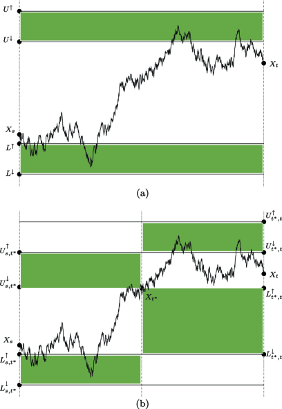
Figure 1: Top panel (a): the intersection layer information $\mathcal{I}_{s,t}$ for a Brownian path. The underlying trajectory starts at $X_{s}$ and finishes at $X_{t}$ with its extrema found in the shaded areas. Bottom panel (b): the bisection of $\mathcal{I}_{s,t}$ into $\mathcal{I}_{s,t^{*}}$ and $\mathcal{I}_{t^{*},t}$. The algorithm simulates $X_{t^{*}}$ and then decides that the extrema for each of the intervals $[s,t^{*}]$ and $[t^{*},t]$ are in the shaded areas, that is, $\mathcal{U}_{s,t^{*}}=[X_{t^{*}},U^{\downarrow}]$, $\mathcal{U}_{t^{*},t}=[U^{\downarrow},U^{\uparrow}]$, $\mathcal{L}_{s,t^{*}}=[L^{\downarrow},L^{\uparrow}]$ and $\mathcal{L}_{t^{*},t}=[L^{\uparrow},X_{t^{*}}]$. The algorithm outputs the upgraded information $\mathcal{I}_{s,t^{*}}=\{X_{s},X_{t^{*}},\mathcal{L}_{s,t^{*}},\mathcal{U}_{s,t^{*}}\}$ and $\mathcal{I}_{t^{*},t}=\{X_{t^{*}},X_{t},\mathcal{L}_{t^{*},t},\mathcal{U}_{t^{*},t}\}$.

2.1 Refining the information $\mathcal{I}_{s,t}$

During the iterations at the execution of the $\varepsilon$-strong algorithm, for each piece of information $\mathcal{I}_{s,t}$ we will need to control the width of the layers $\mathcal{L}_{s,t}$, $\mathcal{U}_{s,t}$ relatively to the size $t-s$ of the time interval to ensure convergence of the bounding paths enveloping the underlying Brownian path. Thus, the refinement of the information $\mathcal{I}_{s,t}$ corresponds to a procedure that updates $\mathcal{I}_{s,t}$ by halving the allowed width for the minimum $m$ or the maximum $M$ of the path, thereby correspondingly updating the layers $\mathcal{L}_{s,t}$ or $\mathcal{U}_{s,t}$.

More analytically, refinement of $\mathcal{I}_{s,t}$ corresponds to deciding whether the minimum $m$ on $[s,t]$, already known to be in $[L^{\downarrow},L^{\uparrow}]$, lies in $[L^{\downarrow},(L^{\downarrow}+L^{\uparrow})/2]$ or $[(L^{\downarrow}+L^{\uparrow})/2,L^{\uparrow}]$, that is, whether $\mathcal{L}_{s,t}$ is equal to $[L^{\downarrow},(L^{\downarrow}+L^{\uparrow})/2]$ or $[(L^{\downarrow}+L^{\uparrow})/2,L^{\uparrow}]$; the apparent analogue of such a consideration applies for the maximum $M$. The analytical method of sampling the relevant binary random variables for carrying out this procedure will be described in Section 5.

2.2 Bisecting the information $\mathcal{I}_{s,t}$

This is a more involved operation on $\mathcal{I}_{s,t}$, and involves bisecting $\mathcal{I}_{s,t}$ into the more analytical information $\mathcal{I}_{s,t^{*}}\vee\mathcal{I}_{t^{*},t}$ for some intermediate time instance $t^{*}\in(t,s)$. In particular, we will be selecting $t^{*}=(t+s)/2$ within the $\varepsilon$-strong algorithm. The method begins by sampling the middle point $X_{t^{*}}$ conditionally on $\mathcal{I}_{s,t}$, and then appropriately sampling the layers for the two pieces of information $\mathcal{I}_{s,t^{*}}$, $\mathcal{I}_{t^{*},t}$. The practicalities of implementing the second part of the method will depend on whether $X_{t^{*}}$ falls within a layer of $\mathcal{I}_{s,t}$ or not, thus we present the bisection operation in more detail in Table 1.

Table 1: The procedure for bisecting the information $\mathcal{I}_{s,t}$. It returns the intersection layers $\mathcal{I}_{s,t^{*}}$ and $\mathcal{I}_{t^{*},t}$ with refined information about the underlying path (compared to $\mathcal{I}_{s,t}$)

Bisect($\mathcal{I}_{s,t}$):

a 1. Set $t^{*}=(t+s)/2$. Simulate $X_{t^{*}}$ given $\mathcal{I}_{s,t}$. Set $U^{\downarrow}=U^{\downarrow}\vee X_{t^{*}}$, $L^{\uparrow}=L^{\uparrow}\wedge X_{t^{*}}$.

2a. Decide if $\mathcal{U}_{s,t^{*}}=[X_{s}\vee X_{t^{*}},U^{\downarrow}]$ or $[U^{\downarrow},U^{\uparrow}]$.

2b. Decide if $\mathcal{U}_{t^{*},t}=[X_{t^{*}}\vee X_{t},U^{\downarrow}]$ or $[U^{\downarrow},U^{\uparrow}]$.

2c. Decide if $\mathcal{L}_{s,t^{*}}=[L^{\downarrow},L^{\uparrow}]$ or $[L^{\uparrow},X_{s}\wedge X_{t^{*}}]$.

2d. Decide if $\mathcal{L}_{t^{*},t}=[L^{\downarrow},L^{\uparrow}]$ or $[L^{\uparrow},X_{t^{*}}\wedge X_{t}]$.

a 3. Return $\mathcal{I}_{s,t^{*}}\vee\mathcal{I}_{t^{*},t}$.

Note that if $X_{t^{*}}>U^{\downarrow}$ the two upper layers (for $\mathcal{I}_{s,t^{*}}$ and $\mathcal{I}_{t^{*},t}$) will be directly set to $[X_{t^{*}},U^{\uparrow}]$, and we will have to simulate extra randomness about the underlying path only to determine the lower layers. Correspondingly, if $X_{t^{*}}<L^{\uparrow}$ the two lower layers will immediately be set to $[L^{\downarrow},X_{t^{*}}]$. In the scenario when $L^{\downarrow}<X_{t^{*}}<U^{\downarrow}$, we will have to simulate extra randomness to determine all four layers. We describe in Section 5 the algorithms for sampling $X_{t^{*}}$ and determining the layers. Figure 1 shows a graphical illustration of the bisection procedure.

3 $\varepsilon$-Strong simulation of Brownian path

We introduce an iterative simulation algorithm with input a Brownian bridge $X$ on the domain $[0,1]$ and output, after $n$ iterations, upper and lower dominating processes $X^{\downarrow}(n)=\{X^{\downarrow}_{u}(n);u\in[0,1]\}$ and $X^{\uparrow}(n)=\{X^{\uparrow}_{u}(n);u\in[0,1]\}$ satisfying the monotonicity and limiting requirements (1) and (2) respectively. Note that $X$ here is a continuous time Brownian bridge path, thus an infinite-dimensional random variable. However, the bounding processes will be piece-wise constant, thus inherently finite-dimensional. One will be able to realise complete sample paths of $X^{\downarrow}(n)$ or $X^{\uparrow}(n)$ on a computer without retreating to any sort of discretization or approximation errors (apart from those due to finite computing accuracy).

3.1 $\varepsilon$-Strong algorithm

Given some initial intersection layer information $\mathcal{I}_{0,1}$, the algorithm will naturally set $X^{\uparrow}_{u}(0)=U^{\uparrow}_{0,1}$ and $X^{\downarrow}_{u}(0)=L^{\downarrow}_{0,1}$ for all instances $u\in[0,1]$. It will then iteratively bisect the acquired intersection layers, as described in Section 2.2, to obtain more information about the underlying sample path on finer time intervals. To ensure convergence of the discrepancy $X^{\uparrow}(n)-X^{\downarrow}(n)$ the algorithm will sometimes refine the information on some intersection layers, as described in Section 2.1, to reduce the uncertainty for the extrema. We give the pseudocode about the algorithm in Table 2.

Table 2: The $\varepsilon$-strong algorithm. It iteratively unveils extra information about the underlying path. It outputs the collection of intersection layers $\mathcal{P}=\bigvee_{j=1}^{2^{n}}\mathcal{I}_{(j-1)2^{-n},j2^{-n}}$

$\varepsilon$-strong($X_{0}$, $X_{1}$, $n$):

1. Initialize $\mathcal{U}_{0,1}$, $\mathcal{L}_{0,1}$, set $\mathcal{I}_{0,1}=\{X_{0},X_{1},\mathcal{U}_{0,1},\mathcal{L}_{0,1}\}$. Set $\mathcal{P}=\{\mathcal{I}_{0,1}\}$ and $i=1$.

2. For each of the $2^{i-1}$ intersection layers in $\mathcal{P}$, say $\mathcal{I}_{s,t}$, do the following:

ii. Bisect the information $\mathcal{I}_{s,t}$ into $\mathcal{I}_{s,t^{*}}$, $\mathcal{I}_{t^{*},t}$, where $t^{*}=(t+s)/2$.

ii. Refine $\mathcal{I}_{s,t^{*}}$, $\mathcal{I}_{t^{*},t}$ until the width of their layers is not greater than $\sqrt{(t-s)/2}$.

3. Collect the updated information, $\mathcal{P}=\bigvee_{j=1}^{2^{i}}\mathcal{I}_{(j-1)2^{-i},j2^{-i}}$.

4. If $i<n$ set $i=i+1$ and return to Step 2; otherwise return $\mathcal{P}$.

Utilising the information the $\varepsilon$-strong algorithm returns, we define the dominating processes as follows:

$$X^{\uparrow}_{u}(n) = \sum_{i=1}^{2^{n}}U^{\uparrow}_{(i-1)2^{-n},i2^{-n}}\cdot\mathrm{I}_{u\in((i-1)2^{-n},i2^{-n}]},$$

$$X^{\downarrow}_{u}(n) = \sum_{i=1}^{2^{n}}L^{\downarrow}_{(i-1)2^{-n},i2^{-n}}\cdot\mathrm{I}_{u\in((i-1)2^{-n},i2^{-n}]}.$$

The square-root rate at Step 2.ii of the algorithm in Table 2 is to guarantee convergence of the dominating paths with minimal computing cost: it provides the correct distribution of effort between time-interval and extrema-interval bisections. To understand this, note that the range of a Brownian motion (or a Brownian bridge) on $[0,2^{-n}]$ scales as $\mathcal{O}(2^{-n/2})$; see, for instance, [18]. Thus, had we used the actual Brownian minima and maxima to define dominating processes for the Brownian path in the way of (3.1) the rate of convergence would have been $\mathcal{O}(2^{-n/2})$; we cannot exceed such a rate, but we can preserve it if our extrema are not further than $\mathcal{O}(2^{-n/2})$ from the actual ones. This intuitive statement will be made rigorous in the sequel, when an explicit result on the rate of convergence of the dominating processes in $L_{1}$-norm is given.

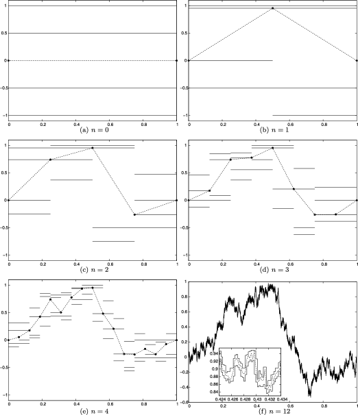
Figure 2: The $\varepsilon$-strong algorithm as applied on a personal computer. For each step $n$, the horizontal black lines show the allowed interval for the minima and the maxima: this information is separately available for all $2^{n}$ time sub-intervals partitioning $[0,1]$. Note that the last graph corresponds to $n=12$, with the subplot in its frame corresponding to a zooming on the position of the paths on the time interval $[0.424,0.434]$.

Figure 2 shows successive steps of the $\varepsilon$-strong algorithm as implemented on a computer. For each $n$, the horizontal black lines show the interval where the maxima and the minima are located: this information is available for all $2^{n}$ sub-intervals bisecting the initial time interval $[0,1]$. The dashed black line corresponds to the linear interpolation of successively unveiled positions of the underlying Brownian path. The last graph (f) corresponds to $n=12$; in this case, we have zoomed on a particular subinterval of $[0,1]$ to be able to visualise the difference between the bounding paths and the underlying Brownian one.

3.2 Convergence properties

Almost sure convergence of the dominating paths follows directly from the continuity of the Brownian path $X$. The analytical proof is given in the following proposition.

Proposition 3.0

Consider the continuous-time processes $X^{\uparrow}(n)$, $X^{\downarrow}(n)$ defined in (3.1). Then, the convergence in supremum norm in (2) will hold in the limit $n\rightarrow\infty$.

[Proof.] For a Brownian bridge $X$ on $[0,1]$, we consider:

$$D_{n}:=\sup_{1\leq i\leq 2^{n}}\bigl{(}M_{(i-1)2^{-n},i2^{-n}}-m_{(i-1)2^{-n},i2^{-n}}\bigr{)}.$$

Uniform continuity implies that, with probability $1$:

$$\lim_{n\rightarrow\infty}D_{n}=0.$$

Now, we have that:

$$\sup_{u\in[0,1]}|X^{\uparrow}_{u}(n)-X^{\downarrow}_{u}(n)|\leq D_{n}+2\cdot 2^{-n/2}\rightarrow 0,$$

where we have used the fact that Step 2.ii of the $\varepsilon$-strong algorithm guarantees that

$$U^{\uparrow}_{(i-1)2^{-n},i2^{-n}} \leq M_{(i-1)2^{-n},i2^{-n}}+2^{-n/2},$$

$$L^{\downarrow}_{(i-1)2^{-n},i2^{-n}} \geq m_{(i-1)2^{-n},i2^{-n}}-2^{-n/2}.$$

A more involved result can give the rate of convergence of the dominating processes and will be of practical significance for the efficiency of Monte Carlo methods based on the $\varepsilon$-strong algorithm.

Proposition 3.0

Consider the $L_{1}$-distance:

$$|X^{\uparrow}(n)-X^{\downarrow}(n)|_{1}=\int_{0}^{1}|X^{\uparrow}_{u}(n)-X^{\downarrow}_{u}(n)|\,\mathrm{d}u.$$

Then:

$$2^{n/2}\times\mathrm{E}[|X^{\uparrow}(n)-X^{\downarrow}(n)|_{1}]=\mathcal{O}(1).$$

[Proof.] We proceed as follows:

$$|X^{\uparrow}(n)-X^{\downarrow}(n)|_{1} = \sum_{i=1}^{2^{n}}\bigl{(}U^{\uparrow}_{(i-1)2^{-n},i2^{-n}}-L^{\downarrow}_{(i-1)2^{-n},i2^{-n}}\bigr{)}\cdot 2^{-n}$$

$$\leq \sum_{i=1}^{2^{n}}\bigl{(}M_{(i-1)2^{-n},i2^{-n}}-m_{(i-1)2^{-n},i2^{-n}}+2\cdot 2^{-n/2}\bigr{)}\cdot 2^{-n},$$

the inequality being a direct consequence of Step 2.ii of the $\varepsilon$-strong algorithm in Table 2. Consider now the path from $X_{(i-1)2^{-n}}$ to $X_{i2^{-n}}$. Let $Z$ be a Brownian bridge from $Z_{0}=0$ to $Z_{2^{-n}}=0$; we denote by $M_{z}$ and $m_{z}$ its maximum and minimum, respectively. Conditionally on $X_{(i-1)2^{-n}}$ and $X_{i2^{-n}}$, a known property of the Brownian bridge implies (see, e.g., [14]) that:

$$X_{t+(i-1)2^{-n}}=Z_{t}+\biggl{(}1-\frac{t}{2^{-n}}\biggr{)}X_{(i-1)2^{-n}}+\frac{t}{2^{-n}}X_{i2^{-n}},\qquad t\in[0,2^{-n}],$$

in the sense that the processes on the two sides of the above equation have the same distribution. It is now clear that:

$$M_{(i-1)2^{-n},i2^{-n}}-m_{(i-1)2^{-n},i2^{-n}}\leq\bigl{|}X_{i2^{-n}}-X_{(i-1)2^{-n}}\bigr{|}+(M_{z}-m_{z}).$$

So, taking expectations at (3.2), we get:

$$\mathrm{E}[|X^{\uparrow}(n)-X^{\downarrow}(n)|_{1}]\leq\mathrm{E}[M_{z}-m_{z}]+2\cdot 2^{-n/2}+\sum_{i=1}^{2^{n}}\mathrm{E}\bigl{|}X_{i2^{-n}}-X_{(i-1)2^{-n}}\bigr{|}2^{-n}$$

The finite-dimensional distributions of the initial Brownian bridge from $X_{0}$ to $X_{1}$ imply that:

$$X_{i2^{-n}}-X_{(i-1)2^{-n}}\sim N\bigl{(}(X_{1}-X_{0})2^{-n},2^{-n}(1-2^{-n})\bigr{)},$$

which gives directly that:

$$\mathrm{E}\bigl{|}X_{i2^{-n}}-X_{(i-1)2^{-n}}\bigr{|}=\mathcal{O}(2^{-n/2}).$$

It remains to show that $\mathrm{E}[M_{z}-m_{z}]=\mathcal{O}(2^{-n/2})$ to complete the proof. Now, self-similarity of Brownian motion implies that:

$$Z_{u}=2^{-n/2}\tilde{Z}_{u/2^{-n}},$$

where $\tilde{Z}$ is a Brownian bridge from $\tilde{Z}_{0}=0$ to $\tilde{Z}_{1}=0$. Let $\tilde{M}_{z}$, $\tilde{m}_{z}$ be the maximum and minimum of $\tilde{Z}$. Due to the self-similarity, we have

$$M_{z}-m_{z}=2^{-n/2}(\tilde{M}_{z}-\tilde{m}_{z}).$$

Since $\tilde{M}_{z}-\tilde{m}_{z}$ in a random variable of finite expectation (see, e.g., [14]), we obtain directly that $\mathrm{E}[M_{z}-m_{z}]=\mathcal{O}(2^{-n/2})$ which completes the proof.

4 The $\zeta$-function

We have yet to present the sampling methods employed when refining or bisecting an intersection layer during the execution of the $\varepsilon$-strong algorithm, thus constituting the building blocks of our algorithm. All probabilities involved in these methods can be expressed in terms of a hitting probability of the Brownian path. We denote by

$$\mathbb{W}^{(l,x,y)}$$

the probability law of a Brownian bridge from $X_{0}=x$ to $X_{l}=y$. Let $\zeta(L,U;l,x,y)$, with $L<U$, be the probability that the Brownian bridge escapes the interval $[L,U]$. That is:

$$\zeta(L,U;l,x,y)=\mathbb{W}^{(l,x,y)}[m_{0,l}<L\mbox{ or }M_{0,l}>U].$$

We also define:

$$\gamma(L,U;l,x,y)=1-\zeta(L,U;l,x,y).$$ (6)

These probabilities can be calculated analytically in terms of an infinite series. The result is based on a partition of Brownian paths w.r.t. to a trace they leave on two bounding lines and can be attributed back to [11]; for more recent references see [1, 17, 9]. We define for $j\geq 1$,

$$\bar{\sigma}_{{}_{j}}(x,y,\delta,\xi) = \exp\biggl{\{}-\frac{2}{l}[\delta j+\xi-x][\delta j+\xi-y]\biggr{\}},$$

$$\bar{\tau}_{{}_{j}}(x,y,\delta) = \exp\biggl{\{}-\frac{2j}{l}[\delta^{2}j+\delta(x-y)]\biggr{\}}.$$

Then, Theorem 3 of [17] yields

$$\zeta(L,U;l,x,y)=\cases{\displaystyle\sum_{j=1}^{\infty}(\sigma_{{}_{j}}-\tau_{{}_{j}}),&\quad$L<x,y<U,$\vspace*{2pt}\cr 1,&\quad$\mbox{otherwise},$}$$ (8)

where

$$\sigma_{j} = \bar{\sigma}_{{}_{j}}(x,y,U-L,L)+\bar{\sigma}_{{}_{j}}(-x,-y,U-L,-U),$$

$$\ \tau_{j} = \bar{\tau}_{{}_{j}}(x,y,U-L)+\bar{\tau}_{{}_{j}}(-x,-y,U-L).\vskip 6.0pt plus 2.0pt minus 2.0pt$$

The infinite series in (8) exhibits a monotonicity property which will be exploited by our simulation algorithms. We consider the sequence $\{S_{n}\}$, with $S_{n}=S_{n}(L,U;l,x,y)$, defined as:

$$S_{2n-1}=\sum_{j=1}^{n-1}(\sigma_{j}-\tau_{j})+\sigma_{n},\qquad S_{2n}=S_{2n-1}-\tau_{n},$$ (10)

when $L<x,y<U$, otherwise $S_{n}\equiv 1$. Then:

$$0<S_{2n}\leq S_{2n+2}\leq\zeta\leq S_{2n+1}\leq S_{2n-1}$$ (11)

for all $n\geq 1$; for a proof see [9] or [5].

4.1 $\zeta$-Derived events

We can combine $\zeta$-probabilities to calculate other conditional probabilities arising in the context of the $\varepsilon$-strong algorithm. We begin with the following definition:

$$\beta(L^{\downarrow},L^{\uparrow},U^{\downarrow},U^{\uparrow};l,x,y):=\mathbb{W}^{(l,x,y)}[L^{\downarrow}<m_{0,l}<L^{\uparrow},U^{\downarrow}<M_{0,l}<U^{\uparrow}].$$

Now, we have the set equality:

$$\{L^{\downarrow}<m_{0,l}<L^{\uparrow},U^{\downarrow}<M_{0,l}<U^{\uparrow}\}$$

(12)

$$\quad=\{L^{\downarrow}<m_{0,l},M_{0,l}<U^{\uparrow}\}-\{L^{\uparrow}<m_{0,l},M_{0,l}<U^{\uparrow}\}\cup\{L^{\downarrow}<m_{0,l},M_{0,l}<U^{\downarrow}\}.\qquad$$

Thus, taking probabilities and recalling the definition of $\gamma$ in (8), we find that:

$$\beta(L^{\downarrow},L^{\uparrow},U^{\downarrow},U^{\uparrow};l,x,y) = \gamma(L^{\downarrow},U^{\uparrow};l,x,y)-\gamma(L^{\uparrow},U^{\uparrow};l,x,y)$$

$${}-\gamma(L^{\downarrow},U^{\downarrow};l,x,y)+\gamma(L^{\uparrow},U^{\downarrow};l,x,y).$$

Before the next event, we enrich the notation for the Brownian bridge measure. We define (for $0<q<l$):

$$\mathbb{W}^{(l,x,y)}_{(q,w)}[\cdot]=\mathbb{W}^{(l,x,y)}[\cdot\mid X_{q}=w].$$

We set $r=l-q$. Consider now the conditional probability:

$$\rho(L^{\downarrow},L^{\uparrow},U^{\downarrow},U^{\uparrow};q,r,x,w,y)=\mathbb{W}^{(l,x,y)}_{(q,w)}[L^{\downarrow}<m_{0,l}<L^{\uparrow},U^{\downarrow}<M_{0,l}<U^{\uparrow}].$$

Using again the set equality (4.1), and taking probabilities under $\mathbb{W}^{(l,x,y)}_{(q,w)}$, we obtain:

$$\rho(L^{\downarrow},L^{\uparrow},U^{\downarrow},U^{\uparrow};q,r,x,w,y)=\gamma_{1}\gamma_{2}-\gamma_{3}\gamma_{4}-\gamma_{5}\gamma_{6}+\gamma_{7}\gamma_{8},$$ (14)

where we have defined:

$$\gamma_{1} = \gamma(L^{\downarrow},U^{\uparrow};q,x,w),\qquad\gamma_{2}=\gamma(L^{\downarrow},U^{\uparrow};r,w,y),\qquad\gamma_{3}=\gamma(L^{\uparrow},U^{\uparrow};q,x,w),$$

$$\gamma_{4} = \gamma(L^{\uparrow},U^{\uparrow};r,w,y),\qquad\gamma_{5}=\gamma(L^{\downarrow},U^{\downarrow};q,x,w),\qquad\gamma_{6}=\gamma(L^{\downarrow},U^{\downarrow};r,w,y),$$

$$\gamma_{7} = \gamma(L^{\uparrow},U^{\downarrow};q,x,w),\qquad\gamma_{8}=\gamma(L^{\uparrow},U^{\downarrow};r,w,y).$$

Note that the product terms arise due to the independency of the Brownian bridges on $[0,q]$ and $[q,l]$. We will be using these expressions for $\beta(\cdot;\cdot)$ and $\rho(\cdot;\cdot)$ in the sequel.

4.2 Simulation of $\zeta$-derived events

We will need to be able to decide whether events of probability $\zeta$ have occurred or not. In a simulation context, this corresponds to determining the value of the binary variable $\mathrm{I}_{R<\zeta}$ for $R\sim\operatorname{Un}[0,1]$. With (11) in mind, we define:

$$J=\inf\{n\geq 1\mathchoice{\nobreak\,\colon}{\nobreak\,\colon}{\nobreak\,\colon\;}{\nobreak\,\colon\;}n\mbox{ odd, }S_{n}<R\mbox{ or }n\mbox{ even, }S_{n}>R\}.$$

Due to the alternating monotonicity property (11) of $S_{n}$:

$$\mathrm{I}_{R<\zeta}=\mathrm{I}_{J\ \mathrm{is\ even}}.$$

Thus, we need a.s. finite number of $J$ computations to evaluate $\mathrm{I}_{R<\zeta}$. Note that $S_{n}$ converges to its limit exponentially fast, so $J$ will be of small expectation; one can easily verify that all its moments are finite. Such an approach was also followed in [5].

In a more general context, we will also be required to decide if events of probability $\beta(\cdot;\cdot)$ or $\rho(\cdot;\cdot)$ have taken place or not; we will in fact be considering even more complex events related with the $\zeta$-function. In the most encompassing scenario, when executing our sampling methods, we will be required to compare a given real number $R$ with $Z(\zeta_{1},\zeta_{2},\ldots,\zeta_{m})$ for some given function $Z$, with the different $\zeta_{i}$’s corresponding to different choices of the arguments $l,x,y,L,U$ for $\zeta(\cdot;\cdot)$. Using the monotonicity property (11), we will be able to develop corresponding alternating sequences $S_{n}^{Z}$ such that:

$$S^{Z}_{2n} \leq S^{Z}_{2n+2}\leq Z(\zeta_{1},\zeta_{2},\ldots,\zeta_{m})\leq S^{Z}_{2n+1}\leq S^{Z}_{2n-1};$$

$$\lim_{n\rightarrow\infty}S^{Z}_{n} = Z(\zeta_{1},\zeta_{2},\ldots,\zeta_{m}),$$

and proceed as above. Analytically, we will determine the value of the comparison binary indicator $\mathrm{I}_{R<Z(\zeta_{1},\zeta_{2},\ldots,\zeta_{m})}$ as follows:

Calculate $S_{n}^{Z}$ until the first $n$ such that either $n$ is odd and $S_{n}^{Z}<R$ (whence return $0$) or $n$ is even and $S_{n}^{Z}>R$ (whence return $1$).

5 Distributions and their simulation

We will now describe analytically all simulation algorithms employed at the development of the $\varepsilon$-strong algorithm presented in Table 2. In particular, one has to develop sampling methods to carry out the refinement and bisection (see Section 2) of the intersection layer $\mathcal{I}_{s,t}$. To simplify the presentation, when conditioning on $X_{s}$, $X_{t^{*}}$ or $X_{t}$ we will make the correspondence:

$$x = X_{s},\qquad w=X_{t^{*}},\qquad y=X_{t},$$

$$l = t-s,\qquad q=t^{*}-s,\qquad r=t-t^{*}.$$

5.1 Bisection of $\mathcal{I}_{s,t}$: Sampling the middle point $X_{t^{*}}$

Bisection of $\mathcal{I}_{s,t}=\{X_{s},X_{t},\mathcal{L}_{s,t},\mathcal{U}_{s,t}\}$, with $\mathcal{L}_{s,t}=[L^{\downarrow},L^{\uparrow}]$, $\mathcal{U}_{s,t}=[U^{\downarrow},U^{\uparrow}]$, begins by sampling a point of the Brownian bridge conditionally on the collected information about its minimum and maximum; this is Step 1 of Table 1. Such a conditional distribution is analytically tractable via Bayes’ theorem.

Proposition 5.0

The distribution $\mathbb{W}[X_{t^{*}}\mid\mathcal{I}_{s,t}]$, with $t^{*}\in[s,t]$, has probability density:

$$f(w)\propto\rho(L^{\downarrow},L^{\uparrow},U^{\downarrow},U^{\uparrow};q,r,x,w,y)\times\pi(w)$$

where $\rho(\cdot;\cdot)$ is defined in (14) and

$$\pi(w)=\exp\biggl{\{}-\frac{1}{2}\biggl{(}w-\biggl{(}\frac{r}{l}x+\frac{q}{l}y\biggr{)}\biggr{)}^{2}\Big{/}\biggl{(}\frac{qr}{l}\biggr{)}\biggr{\}}.$$

[Proof.] The function $\pi(w)$ corresponds to the prior (unnormalised) density for the middle point $X_{t}^{*}|X_{s},X_{t}$ which is easily found to be normally distributed with mean and variance as implied by the expression for $\pi(w)$. So, following the definition of $\rho(\cdot;\cdot)$ in (14), the stated result is an application of Bayes’ theorem.

We will develop a method for sampling from $f(w)$. It is easy to construct an alternating series bounding $f(w)$. Let:

$$\zeta_{i}=1-\gamma_{i},\qquad 1\leq i\leq 8,$$

for the eight $\gamma$-functions appearing at the definition of $\rho$ in (14). Let $\{S_{i,n}\}_{n\geq 1}$ be the alternating series (11) for $\zeta_{i}$, for each $1\leq i\leq 8$; that is:

$$0<S_{i,2n}\leq S_{i,2n+2}\leq\zeta_{i}\leq S_{i,2n+1}\leq S_{i,2n-1},$$ (16)

with $\lim_{n\rightarrow\infty}S_{i,n}=\zeta_{i}$. Consider the sequence $\{S_{n}^{Z}\}$ defined as follows:

$$S_{n}^{Z} = (1-S_{1,n+1}-S_{2,n+1}+S_{1,n}S_{2,n})-(1-S_{3,n}-S_{4,n}+S_{3,n+1}S_{4,n+1})$$

$${}-(1-S_{5,n}-S_{5,n}+S_{5,n+1}S_{6,n+1})+(1-S_{7,n+1}-S_{8,n+1}+S_{7,n}S_{8,n}).$$

Due to (16), one can easily verify that $\{S_{n}^{Z}\}$ is an alternating sequence for $\rho(\cdot;\cdot)$, in the sense that:

$$S^{Z}_{2n}\leq S^{Z}_{2n+2}\leq\rho(L^{\downarrow},L^{\uparrow},U^{\downarrow},U^{\uparrow},q,r,x,w,y)\leq S^{Z}_{2n+1}\leq S^{Z}_{2n-1}$$ (18)

with $\lim_{n\rightarrow\infty}S^{Z}_{n}=\rho(L^{\downarrow},L^{\uparrow},U^{\downarrow},U^{\uparrow};q,r,x,w,y)$.

We exploit this structure to build a rejection sampler to draw from the density $f(w)$ in Proposition 3. We will use proposals from:

$$f_{2n+1}(w)=S_{2n+1}^{Z}(w)\times\pi(w),$$

where we have emphasized the dependence of $S^{Z}_{2n+1}$ on the argument $w$. Note that the domain of both $f(w)$, $f_{2n+1}(w)$ is $[L^{\downarrow},U^{\uparrow}]$. Now, we will illustrate that $S^{Z}_{2n+1}(w)$ has a concrete structure that we will exploit for our sampler. Consider the first of the four terms forming up $S^{Z}_{2n+1}$ from (5.1):

$$1-S_{1,2n+2}-S_{2,2n+2}+S_{1,2n+1}S_{2,2n+1}.$$ (19)

Following the analytical definition of the alternating sequences in equations (4), (4), (10), both $S_{1,n}$ and $S_{2,n}$, can be expressed as a sum of $2n$ terms each having the exponential structure $\pm\exp\{a+bw\}\mathrm{I}_{L^{\downarrow}<w<U^{\uparrow}}$ for appropriate constants $a,b$ varying among the $2n$ terms. Thus, the quantity in (19) can be expressed as:

$$1+\sum_{i=1}^{k_{1,n}}(-1)^{c_{i}}\exp\{a_{i}+b_{i}w\}\mathrm{I}_{L^{\downarrow}<w<U^{\uparrow}}$$

for $k_{1,n}=4\{(2n+1)^{2}+(2n+2)\}$, and constants $a_{i}$, $b_{i}$, $c_{i}$ with $c_{i}\in\{0,1\}$. Working similarly for all four summands forming up $S^{Z}_{2n+1}$ in (5.1), we get that the function $f_{2n+1}(w)$ can in fact be written as the weighted sum:

$$f_{2n+1}(w)=\sum_{i=1}^{k_{n}}(-1)^{c_{i}}\exp\{a_{i}+b_{i}w\}\mathrm{I}_{L_{i}<w<U_{i}}\times\pi(w)$$ (20)

for $k_{n}=2(k_{1,n}+k_{2,n})$ with $k_{2,n}=4\{(2n+2)^{2}+(2n+1)\}$, and some explicit constants $a_{i}$, $b_{i}$, $c_{i}\in\{0,1\}$, $L_{i}$, $U_{i}$. Experimentation has showed that $f_{1}$ is already a very good envelope function for the rejection sampler, in which case $k_{n}\equiv k_{0}=64$; this is not accidental, and relates with the rapid exponential convergence of the alternating sequence in (10) to its limit. The cdf, say $F_{1}(w)$, corresponding to the unormalised density function $f_{1}(w)$ can be analytically identified since integrals for each of the summands in (20) can be expressed as differences of the cdf of the standard Gaussian distribution. Samples from $f_{1}(w)$ can then be generated using the inverse cdf method, that is, by returning $F_{1}^{-1}(R)$ for $R\sim\operatorname{Un}[0,1]$. $F_{1}^{-1}$ cannot be found analytically, but numerical methods can return $F_{1}^{-1}(R)$, up to maximum allowed computer accuracy, exponentially fast. We have used MATHEMATICA to automatically calculate all integrals giving the cdf, and then incorporated the calculation into a C++ code.

Summarising, our rejection sampler will be as described below, where for simplicity we write $\rho(w)\equiv\rho(L^{\downarrow},L^{\uparrow},U^{\downarrow},U^{\uparrow};q,r,x,w,y)$:

Repeat until the first accepted draw:

Propose $w\sim f_{1}$ and accept with probability $f(w)/f_{1}(w)\equiv\rho(w)/S^{Z}_{1}(w)$.

Note here that the acceptance probability involves $\rho(w)$ which is made up of eight infinite series, see (14). We avoid approximations by using the alternating construction (18) and employ the methods of Section 4.2 to obtain the value of the decision indicator $\mathrm{I}_{R<\rho(w)/S^{Z}_{1}(w)}$ for some $R\sim\operatorname{Un}[0,1]$.

As shown in Step 1 of Table 1, once $X_{t^{*}}$ is obtained, we adjust the allowed range for the extrema of the bridge on $[s,t]$ by simply setting $U^{\downarrow}=U^{\downarrow}\vee X_{t^{*}}$, $L^{\uparrow}=L^{\uparrow}\wedge X_{t^{*}}$.

5.2 Bisection of $\mathcal{I}_{s,t}$: Updating the Layers given $X_{t^{*}}$

At the second step of the bisection procedure, see Table 1, we obtain separate information for the extrema of the two newly formed bridges given the middle point $X_{t^{*}}$: the one bridge being from $X_{s}$ to $X_{t^{*}}$, the other from $X_{t^{*}}$ to $X_{t}$. In particular, the algorithm will decide over the range of the four newly formed layers, $\mathcal{L}_{s,t^{*}}$, $\mathcal{U}_{s,t^{*}}$, $\mathcal{L}_{t^{*},t}$, $\mathcal{U}_{t^{*},t}$ in the following manner: for the case of $\mathcal{L}_{s,t^{*}}$ for instance a decision will be made over whether $m_{s,t^{*}}$ lies in $[L^{\downarrow},L^{\uparrow}]$ (which is the allowed range for the minimum of the original bridge on $[s,t]$) or in $[L^{\uparrow},X_{s}\wedge X_{t^{*}}]$. The apparent analogues apply in the case of the three other layers.

One might initially think that there are in total $2^{4}$ different scenaria for the four layers. But one has to remember that the update has to respect the information in $\mathcal{I}_{s,t}$, so that at least one of the two minima (resp. maxima) on $[s,t^{*}]$ and $[t^{*},t]$ must lie in $[L^{\downarrow},L^{\uparrow}]$ (resp. $[U^{\downarrow},U^{\uparrow}]$). In particular, there are in fact nine different possible scenaria, which are the ones shown in Table 3 (labelled as events $\{E=i\}$, for $1\leq i\leq 9$): a value of $1$ in Table 3 means that the corresponding minimum or maximum will still be found within the allowed range for the original bridge on $[s,t]$, whereas a value of $0$ means that the second option occurs and the extremum will be shifted inwards. For instance, a value of $0$ for the indicator variable concerning $m_{s,t^{*}}$, $M_{s,t^{*}}$, $m_{t^{*},t}$ or $M_{t^{*},t}$ implies that $m_{s,t^{*}}\in[L^{\uparrow},X_{s}\wedge X_{t^{*}}]$, $M_{s,t^{*}}\in[X_{s}\vee X_{t^{*}},U^{\downarrow}]$, $m_{t^{*},t}\in[L^{\uparrow},X_{t^{*}}\wedge X_{t}]$ or $M_{t^{*},t}\in[X_{t^{*}}\vee X_{t},U^{\downarrow}]$, respectively.

Table 3: The nine possible scenaria for the extrema of the two Brownian bridges (from $X_{s}$ to $X_{t}^{*}$ and from $X_{t^{*}}$ to $X_{t}$)

	Left bridge		Right bridge
Event
$E=i$	$\mathrm{I}_{m_{s,t^{*}}\in[L^{\downarrow},L^{\uparrow}]}$	$\mathrm{I}_{M_{s,t^{*}}\in[U^{\downarrow},U^{\uparrow}]}$	$\mathrm{I}_{m_{t^{*},t}\in[L^{\downarrow},L^{\uparrow}]}$	$\mathrm{I}_{M_{t,t^{*}}\in[U^{\downarrow},U^{\uparrow}]}$
$i=1$	$1$	$1$	$1$	$1$
$i=2$	$1$	$1$	$0$	$1$
$i=3$	$1$	$1$	$1$	$0$
$i=4$	$1$	$1$	$0$	$0$
$i=5$	$0$	$1$	$1$	$1$
$i=6$	$0$	$1$	$1$	$0$
$i=7$	$1$	$0$	$1$	$1$
$i=8$	$1$	$0$	$0$	$1$
$i=9$	$0$	$0$	$1$	$1$

=285pt $i$ $\mathrm{P}[E=i|\mathcal{I}_{s,t},X_{t^{*}}]\times\rho(L^{\downarrow},L^{\uparrow},U^{\downarrow},U^{\uparrow};q,r,x,w,y)$ 1 $\beta(L^{\downarrow},L^{\uparrow},U^{\downarrow},U^{\uparrow};q,x,y)\times\beta(L^{\downarrow},L^{\uparrow},U^{\downarrow},U^{\uparrow};r,w,y)$ 2 $\beta(L^{\downarrow},L^{\uparrow},U^{\downarrow},U^{\uparrow};q,x,w)\times\beta(L^{\uparrow},w_{y},U^{\downarrow},U^{\uparrow};r,w,y)$ 3 $\beta(L^{\downarrow},L^{\uparrow},U^{\downarrow},U^{\uparrow};q,x,w)\times\beta(L^{\downarrow},L^{\uparrow},w^{y},U^{\downarrow};r,w,y)$ 4 $\beta(L^{\downarrow},L^{\uparrow},U^{\downarrow},U^{\uparrow};q,x,w)\times\beta(L^{\uparrow},w_{y},w^{y},U^{\downarrow};r,w,y)$ 5 $\beta(L^{\uparrow},w_{x},U^{\downarrow},U^{\uparrow};q,x,w)\times\beta(L^{\downarrow},L^{\uparrow},U^{\downarrow},U^{\uparrow};r,w,y)$ 6 $\beta(L^{\downarrow},L^{\uparrow},U^{\downarrow},U^{\uparrow};q,x,w)\times\beta(L^{\downarrow},L^{\uparrow},U^{\downarrow},U^{\uparrow};r,w,y)$ 7 $\beta(L^{\uparrow},w_{x},U^{\downarrow},U^{\uparrow};q,x,w)\times\beta(L^{\downarrow},L^{\uparrow},w^{y},U^{\downarrow};r,w,y)$ 8 $\beta(L^{\downarrow},L^{\uparrow},w^{x},U^{\downarrow};q,x,w)\times\beta(L^{\uparrow},w_{y},U^{\downarrow},U^{\uparrow};r,w,y)$ 9 $\beta(L^{\uparrow},w_{x},w^{x},U^{\downarrow};q,x,w)\times\beta(L^{\downarrow},L^{\uparrow},U^{\downarrow},U^{\uparrow};r,w,y)$

Table 4: The conditional probabilities for each of the events in Table 3

The probability for each of the events in Table 3 can be derived via functions $\beta(\cdot;\cdot)$ and $\rho(\cdot;\cdot)$ defined in (4.1) and (14), respectively. Recall that we are conditioning upon $\mathcal{I}_{s,t}$ and $X_{t^{*}}$, so we work as follows:

$$\mathrm{P}[E=i|\mathcal{I}_{s,t},X_{t^{*}}] = \mathrm{P}[E=i|m\in[L^{\downarrow},L^{\uparrow}],M\in[U^{\downarrow},U^{\uparrow}],X_{s},X_{t^{*}},X_{t}]$$

$$= \frac{\mathrm{P}[E=i,m\in[L^{\downarrow},L^{\uparrow}],M\in[U^{\downarrow},U^{\uparrow}]|X_{s},X_{t^{*}},X_{t}]}{\mathrm{P}[m\in[L^{\downarrow},L^{\uparrow}],M\in[U^{\downarrow},U^{\uparrow}]|X_{s},X_{t^{*}},X_{t}]}$$

$$= \frac{\mathrm{P}[E=i|X_{s},X_{t^{*}},X_{t}]}{\rho(L^{\downarrow},L^{\uparrow},U^{\downarrow},U^{\uparrow};q,r,x,w,y)}.$$

Now, conditionally on $\{X_{s},X_{t^{*}},X_{t}\}$ the law of the path factorises into two independent Brownian bridges. Thus, recalling also the definition of $\beta(\cdot;\cdot)$ in (4.1), the probability $\mathrm{P}[E=i|X_{s},X_{t^{*}},X_{t}]$ in the numerator above can be written as a product of two $\beta(\cdot;\cdot)$ functions. The analytical calculation of the numerator, or equivalently of the product $\mathrm{P}[E=i|\mathcal{I}_{s,t},X_{t^{*}}]\times\rho(L^{\downarrow},L^{\uparrow},U^{\downarrow},U^{\uparrow};q,r,x,w,y)$, is given in Table 4 where, to simplify the presentation, we have set:

$$w_{x}=x\wedge w,\qquad w^{x}=x\vee w,\qquad w_{y}=w\wedge y,\qquad w^{y}=w\vee y.$$

The method to simulate the discrete random variable $E$ could follow the alternating series approach of Section 4.2. Analytically, consider the cumulative probability values $p_{i}=\mathrm{P}[E\leq i|\mathcal{I}_{s,t},X_{t^{*}}]$. A simple inverse cdf sampling method requires finding the index $\inf\{i\geq 1\mathchoice{\nobreak\,\colon}{\nobreak\,\colon}{\nobreak\,\colon\;}{\nobreak\,\colon\;}R<p_{i}\}$ for a $R\sim\operatorname{Un}[0,1]$. Note now that the $p_{i}$’s can be bounded above and below by monotone converging sequences as in (4.2), thus each comparison $\{R<p_{i}\}$ can be carried out via the alternating series approach of Section 4.2 without any need for approximations.

5.3 Remaining sampling procedures

A sampling algorithm is required for the refinement of the uncertainty over the extrema of a Brownian bridge. As described in Section 2.1, given the current intersection layer information $\mathcal{I}_{s,t}$ and in particular the fact that $M_{s,t}\in[L^{\downarrow},L^{\uparrow}]$, the algorithm will need to decide whether the maximum $M_{s,t}$ lies in $[U^{\downarrow},U^{*}]$ or in $[U^{*},U^{\uparrow}]$, for $U^{*}=(U^{\downarrow}+U^{\uparrow})/2$. Recalling the definition of $\beta(\cdot;\cdot)$ from (4.1), it is easy to check that the ratio:

$$\frac{\beta(L^{\downarrow},L^{\uparrow},U^{*},U^{\uparrow};l,x,y)}{\beta(L^{\downarrow},L^{\uparrow},U^{\downarrow},U^{\uparrow};l,x,y)}$$

provides precisely the probability of the event $\{M_{s,t}\in[U^{*},U^{\uparrow}]|\mathcal{I}_{s,t}\}$. Thus, we can again use the alternating sequence construction of Section 4.2 to simulate, without approximation, the binary variable $\mathrm{I}_{M_{s,t}\in[U^{*},U^{\uparrow}]}$. The same approach can be followed for refining the allowed range for the minimum $m_{s,t}$.

We should also give some details over the initialization of the layers $\mathcal{U}_{0,1}$ and $\mathcal{L}_{0,1}$ at the first step of the $\varepsilon$-strong algorithm in Table 2 given $X_{0}$ and $X_{1}$. (Note that sometimes, as in the example applications that we consider in the following section, this initialization steps might not even be necessary, as the problem at hand provides a natural definition of $\mathcal{U}_{0,1}$ and $\mathcal{L}_{0,1}$.) One way to proceed is by specifying increasing sequences $\{a_{i}\}_{i\geq 0}$, $\{b_{i}\}_{i\geq 0}$, with $a_{0}=b_{0}=0$, growing to $\infty$ and a bivariate index $I$ such that:

$$\{I=(i,j)\}=\{\bar{x}-a_{i}<m\leq\bar{x}-a_{i-1},\bar{y}+b_{j-1}<M\leq\bar{y}+b_{j}\},$$

where $\bar{x}=x\wedge y$, $\bar{y}=x\vee y$. We can easily identify the probability distribution of $I$ under the Brownian bridge dynamics since:

$$\mathbb{W}^{(1,x,y)}[I=(i,j)]=\beta(\bar{x}-a_{i},\bar{x}-a_{i-1},\bar{y}+b_{j-1},\bar{y}+b_{j};1,x,y).$$

Thus, we can work as in the case of the simulation of the discrete variable $E$ in Section 5.2: assuming $\tilde{I}=1,2,\ldots$ is some chosen ordering of the states of $I$, an inverse cdf method would required finding $\inf\{i\geq 1\mathchoice{\nobreak\,\colon}{\nobreak\,\colon}{\nobreak\,\colon\;}{\nobreak\,\colon\;}R<\mathrm{P}[I\leq i]\}$ for $R\sim\operatorname{Un}[0,1]$, and approximations at the comparison between $R$ and $\mathrm{P}[I\leq i]$ can be avoided via the alternating series approach. In practice, one could select some big enough values for the first couple of elements of the sequences $\{a_{i}\}$ and $\{b_{i}\}$ so that almost all probability mass is concentrated on $\{I=(i,j)\}$ for $i,j\leq 2$, and not a lot of computational resources are spent on this step.

6 Application: Unbiased estimation of path expectations

The information provided by the $\varepsilon$-strong algorithm can be exploited to deliver unbiased estimators for path expectations arising in applications, avoiding discretization errors characterising standard approaches. We emphasize that we mean to sketch here only a potential direction for application of the algorithm. Analytically, consider a nonnegative path functional $F\mathchoice{\nobreak\,\colon}{\nobreak\,\colon}{\nobreak\,\colon\;}{\nobreak\,\colon\;}C([0,1],\mathbb{R})\mapsto\mathbb{R}^{+}$ and the expectation: $\mathrm{E}[F(X)]$, $X$ being a Brownian motion on $[0,1]$. One can easily check, by integrating out $E$, that:

$$\mathrm{I}_{F(X)>E}\cdot\mathrm{e}^{E},\qquad E\sim\mathrm{Exp}(1),$$ (21)

with $E$ being independent of $X$, is an unbiased estimator of $\mathrm{E}[F(X)]$. The $\varepsilon$-strong algorithm could be utilised here to unbiasedly obtain the value of the binary variable $\mathrm{I}_{F(X)>E}$ in finite computations. We can easily find the second moment of the unbiased estimator in (21):

$$\mathrm{E}\bigl{[}\mathrm{I}_{F(X)>E}\cdot\mathrm{e}^{2E}\bigr{]}=\mathrm{E}\bigl{[}\mathrm{e}^{F(X)}\bigr{]}-1.$$ (22)

We describe for a moment in more detail the identification of $\mathrm{I}_{F(X)>U}$ via the $\varepsilon$-strong algorithm. Utilising the lower and upper convergent processes $X^{\downarrow}(n)$, $X^{\uparrow}(n)$ in (3.1) one could in many cases analytically identify quantities $F^{\downarrow}_{n}$, $F^{\uparrow}_{n}$ (realisable with finite computations) such that:

$$\displaystyle F^{\downarrow}_{n}\leq F^{\downarrow}_{n+1}\leq F(X)\leq F^{\uparrow}_{n+1}\leq F^{\uparrow}_{n};$$

$$\displaystyle F^{\uparrow}_{n}-F^{\downarrow}_{n}\rightarrow 0.$$

Given enough iterations, there will be agreement; for the a.s. finite random instance:

$$\kappa=\inf\{n\geq 0\colon\ \mathrm{I}_{F^{\downarrow}_{n}>E}=\mathrm{I}_{F^{\uparrow}_{n}>E}\}$$ (23)

we will have

$$\mathrm{I}_{F(X)>E}=\mathrm{I}_{F^{\downarrow}_{\kappa}>E}.$$ (24)

Thus, combining (21) with (24), we have developed an unbiased estimator of a path expectation, involving finite computations. Certainly, the numerical efficiency of such an estimation will rely heavily on the stochastic properties of $\kappa$ and the cost of generating $F^{\downarrow}_{n}$, $F^{\uparrow}_{n}$, and of course the variance of the estimator.

The particular derivation of the above unbiased estimator of the path expectation is by no means restrictive; one can generate unbiased estimators using distributions other than the exponential. Consider the following scenario. We can generate some preliminary bounds $F^{\downarrow}_{n_{0}}$, $F^{\uparrow}_{n_{0}}$ up to some fixed or random (depending on $X$) instance $n_{0}$. Now, one can easily check (by considering the conditional expectation w.r.t. $R|X$) that:

$$\mathrm{I}_{F(X)>R}F^{\uparrow}_{n_{0}}+\mathrm{I}_{F(X)<R}F^{\downarrow}_{n_{0}};\qquad R\sim\operatorname{Un}[F^{\downarrow}_{n_{0}},F^{\uparrow}_{n_{0}}],$$ (25)

is also an unbiased estimator of $\mathrm{E}[F(X)]$. We have empirically found the estimator (25) to be much more robust than (21) in the numerical applications we present in the sequel. This is not accidental: for instance, considering a random $n_{0}$ such that $F^{\uparrow}_{n_{0}}-F^{\downarrow}_{n_{0}}<C$, for a constant $C>0$, we get that the second moment of the estimator (25) will be:

$$\mathrm{E}\bigl{[}\mathrm{I}_{F(X)>R}(F^{\uparrow}_{n_{0}})^{2}+\mathrm{I}_{F(X)<R}(F^{\downarrow}_{n_{0}})^{2}\bigr{]}$$

$$\qquad=\mathrm{E}[F(X)(F^{\uparrow}_{n_{0}}+F^{\downarrow}_{n_{0}})]-\mathrm{E}[F^{\uparrow}_{n_{0}}F^{\downarrow}_{n_{0}}]\leq\mathrm{E}[F^{2}(X)]+C\mathrm{E}[F(X)]$$

which has now a quadratic structure – compare this with (22). In general, increasing $n_{0}$ adds to the computational cost per sample, but decreases the variance. We have empirically found that moderate values of $n_{0}$ deliver significantly better estimates than (21) and will be using such an approach for our numerical examples in the sequel.

6.1 Numerical illustrations

We will apply the $\varepsilon$-strong algorithm to unbiasedly estimate some option prices arising in finance. In particular, option prices are expressed as expectations:

$$\mathrm{E}[F(S)]$$

of a functional $F(\cdot)$ of the path process $S=\{S_{t}\}$ modelling the underlying asset. We will consider some double-barrier options corresponding the expectations of the functionals:

$$F_{a}(S) = \mathrm{e}^{-rT}(\sup S_{t}-K_{S})^{+}\mathrm{I}_{L_{S}<\inf S_{t}<\sup S_{t}<U_{S}};$$ (26)

$$F_{b}(S) = \mathrm{e}^{-rT}\biggl{(}\frac{1}{T}\int_{0}^{T}S_{t}\,\mathrm{d}t-K_{S}\biggr{)}^{+}\mathrm{I}_{L_{S}<\inf S_{t}<\sup S_{t}<U_{S}};$$ (27)

$$F_{c}(S) = \mathrm{e}^{-rT}(\sup S_{t}-K_{S})^{+}\mathrm{I}_{L_{S}<\inf S_{t}\mathrm{e}^{-rt}<\sup S_{t}\mathrm{e}^{-rt}<U_{S}}$$ (28)

(where for $x\in\mathbb{R}$, $x^{+}:=x\vee 0$) for underlying asset $S=\{S_{t};t\in[0,T]\}$ modelled via a geometric Brownian motion (we consider a Black and Scholes framework) determined as:

$$\log S_{t}=\log S_{0}+\biggl{(}r-\frac{\sigma^{2}}{2}\biggr{)}t+\sigma W_{t}$$ (29)

for constants $r$ (interest rate), $\sigma>0$ (volatility) and a Brownian motion $\{W_{t}\}$. Also, $T$ above is the maturity time, $K_{S}$ the strike price and $L_{S}$, $U_{S}$ the lower and upper barriers respectively; suprema and infima are considered over the time period $[0,T]$. Note that $\mathrm{E}[F_{b}(S)]$ corresponds to the price of the Asian option, see, for example, [21]. The process $S_{t}$ is an 1–1 transformation of a Brownian motion with drift. In particular, we can rewrite the functionals (26)–(28) as follows:

$$F_{a}(X) = \mathrm{e}^{-rT}(\mathrm{e}^{\sigma\sup X_{t}}-K_{S})^{+}\mathrm{I}_{L<\inf X_{t}<\sup X_{t}<U};$$ (30)

$$F_{b}(X) = \mathrm{e}^{-rT}\biggl{(}\frac{1}{T}\int_{0}^{T}\mathrm{e}^{\sigma X_{t}}\mathrm{d}t-K_{S}\biggr{)}^{+}\mathrm{I}_{L<\inf X_{t}<\sup X_{t}<U};$$ (31)

$$F_{c}(X) = \mathrm{e}^{-rT}\bigl{(}\mathrm{e}^{\sigma\sup(({r}/{\sigma})t+X_{t})}-K_{S}\bigr{)}^{+}\mathrm{I}_{L<\inf X_{t}<\sup X_{t}<U},$$ (32)

for $L=\log(L_{S})/\sigma$, $U=\log(U_{S})/\sigma$, and:

$$\mathrm{Case}\ F_{a},F_{b}\mathchoice{\nobreak\,\colon}{\nobreak\,\colon}{\nobreak\,\colon\;}{\nobreak\,\colon\;} \qquad X_{t}=\log(S_{0})/\sigma+\biggl{(}\frac{r}{\sigma}-\frac{\sigma}{2}\biggr{)}t+W_{t};$$

$$\mathrm{Case}\ F_{c}\mathchoice{\nobreak\,\colon}{\nobreak\,\colon}{\nobreak\,\colon\;}{\nobreak\,\colon\;} \qquad X_{t}=\log(S_{0})/\sigma-\frac{\sigma}{2}t+W_{t}.$$

Conditionally on its ending point, the dynamics of the drifted Brownian motion do not depend on the value of the drift and coincide with those of a simple Brownian bridge; this is a simple by-product of the Girsanov theorem, see, for example, [15]. Thus, the $\varepsilon$-strong algorithm can now deliver convergent, lower and upper dominating processes for $X$.

The choices of functionals in (26)–(28) is not accidental: some generic characteristics of the structure of each functional (relevant also for other applications) will effect the set-up of the $\varepsilon$-strong algorithm and its efficiency; we will say more on this in the sequel.

For all three examples, our general methodology is as follows: we begin by sampling $X_{T}$ and, then, the indicator variable $\mathrm{I}_{L<\inf X_{t}<\sup X_{t}<U}$; if the latter is $0$ the sample for our unbiased estimator is simply $0$, otherwise we proceed with applying the methods of the $\varepsilon$-strong algorithm by initializing the first intersection layer as $\mathcal{I}_{0,T}=\{X_{0},X_{T},\mathcal{U}_{0,T},\mathcal{L}_{0,T}\}$ for intervals $\mathcal{U}_{0,T}=[X_{0}\vee X_{T},U]$ and $\mathcal{L}_{0,T}=[L,X_{0}\wedge X_{T}]$. In some cases we might not need all of the machinery of the $\varepsilon$-strong algorithm to construct the sequences $F^{\downarrow}_{n}$, $F^{\uparrow}_{n}$ enveloping $F(X)$, with direct implications on the efficiency of the algorithm, as we explain analytically below.

$F_{a}$-example: Only refinement

Here, we need information only on the marginal variable $\sup X_{t}$ (and not the whole of the continuous path on $[0,T]$) to develop an alternating series for $F_{a}(X)$. Thus, it suffices to apply a reduced version of the complete $\varepsilon$-strong algorithm in Table 2 where we only repeatedly refine the initial intersection layer $\mathcal{I}_{0,T}$ (in particular, we only refine the layer for the maximum) as described in Section 2.1 (and never bisect it) to construct $F^{\downarrow}_{n}$, $F^{\uparrow}_{n}$. In particular, having defined:

$$\phi(x)=\mathrm{e}^{-rT}(\mathrm{e}^{\sigma x}-K_{S})^{+}$$

knowing that after $n$ refinements the allowed range for $\sup X_{t}$ is $[U^{\downarrow}_{n},U^{\uparrow}_{n}]$ (with initial position $[U^{\downarrow}_{0},U^{\uparrow}_{0}]=[X_{0}\vee X_{T},U]$) we set $F^{\downarrow}_{n}=\phi(U^{\downarrow}_{n})$, $F^{\uparrow}_{n}=\phi(U^{\uparrow}_{n})$.

$F_{b}$-example: Refinement and bisection

The complete machinery of the $\varepsilon$-strong algorithm in Table 2 is required here as we need to bound a path integral. Recall that the $n$th step of the algorithm provides the piecewise constant paths $X^{\downarrow}_{t}(n)$, $X^{\uparrow}_{t}(n)$ enveloping $X$ defined in (3.1). We now set $F^{\downarrow}_{n}=F_{b}(X^{\downarrow}(n))$, $F^{\uparrow}_{n}=F_{b}(X^{\uparrow}(n))$.

$F_{c}$-example: Selective refinement and bisection

We will now only need to bisect a selection of intersection layers as we will be allowed to delete intersection layers that cannot definitely contain $\sup(\frac{r}{\sigma}t+X_{t})$ during the execution of the $\varepsilon$-strong algorithm. In particular, assuming the current collection (after $n-1$ steps) of stored intersection layers $\mathcal{I}_{s_{i},t_{i}}$, with $s_{i}<t_{i}\leq s_{i+1}$, containing information about the path $X$, and determining the allowed range for $\sup(\frac{r}{\sigma}t+X_{t})$ :

$$[U^{\downarrow}_{n-1},U^{\uparrow}_{n-1}]=\biggl{[}\sup_{i}\biggl{\{}U^{\downarrow}_{s_{i},t_{i}}+\frac{r}{\sigma}s_{i}\biggr{\}},\sup_{i}\biggl{\{}U^{\uparrow}_{s_{i},t_{i}}+\frac{r}{\sigma}t_{i}\biggr{\}}\biggr{]}$$ (33)

we proceed to the $n$th step where: (i) we bisect and refine all stored intersection layers $\mathcal{I}_{s_{i},t_{i}}$, (ii) calculate the running bounds $[U^{\downarrow}_{n},U^{\uparrow}_{n}]$ by taking the suprema as in (33) but now over all newly obtained intersection layers, (iii) delete the obtained intersection layers $\mathcal{I}_{s,t}$ for which $U^{\uparrow}_{s,t}<U^{\downarrow}_{n}$ (as they cannot offer extra information on the whereabouts of $\sup(\frac{r}{\sigma}t+X_{t})$ given that we already know that the latter is within $[U^{\downarrow}_{n},U^{\uparrow}_{n}]$) and store only the remaining ones for the next iteration. At each step, we set $F^{\downarrow}_{n}=\phi(U^{\downarrow}_{n})$, $F^{\uparrow}_{n}=\phi(U^{\uparrow}_{n})$ with $\phi$ as defined above.

Numerics

We have run the $\varepsilon$-strong algorithm for the above scenaria. To give an idea of its computing cost, we compare its execution times with those of the standard (Euler) approximation method that replaces the continuous-time path $\{S_{t};t\in[0,T]\}$ with its discretised approximation $\{S_{t_{i}}\}_{i=0}^{l}$, for $t_{i}=t_{i-1}+\delta$, with step-size $\delta=T/l$; then, continuous-time maxima and integrals appearing in the functionals (26)–(28) are replaced with their obvious approximations based on the discrete-time vector $\{S_{t_{i}}\}$. We run our simulations under the parameter selections:

$$r=0.05,\qquad\sigma=0.2,\qquad S_{0}=1,\qquad K=1,\qquad T=1,\qquad U=1.25,\qquad L=0.75.$$

Tables 5–7 show results from the simulation study. For each different algorithm, we show its execution time (all algorithms were coded in C++) and a 95% confidence interval for the mean of the realised estimators to give an idea about the variance of the estimates and their bias (for the case of the Euler approximation, as the $\varepsilon$-strong algorithm is unbiased). The results in Tables 5, 7 are obtained via 100 000 independent realizations of the estimators, whereas those in Table 6 via 10 000 independent realizations.

Table 5: Simulation results from the application of the Euler approximation and the $\varepsilon$-strong algorithm for the estimation of the option price in $\mathrm{E}[F_{a}(S)]$ in (26). The results in the table correspond to a sample of $100\,000$ estimates. $\delta$ is the discretisation increment of the Euler method, and $n_{0}$ is the number of preliminary steps for the $\varepsilon$-strong algorithm before the simulation of the uniform random variable (see (25))

Euler approximation $\delta$ Time (secs) 95% Conf. Int. 1$/$10 0.4 $[638,647]\times 10^{-4}$ 1$/$20 0.8 $[657,667]\times 10^{-4}$ 1$/$40 1.5 $[669,679]\times 10^{-4}$ 1$/$80 2.9 $[674,683]\times 10^{-4}$ 1$/$160 5.8 $[680,689]\times 10^{-4}$

$\varepsilon$-strong $n_{0}$ Time (secs) 95% Conf. Int. 2 1.1 $[683,693]\times 10^{-4}$

Table 6: Similar results as for Table 5, but now for the case of the Asian option $\mathrm{E}[F_{b}(S)]$ in (27) – with the difference that here the results correspond to a sample of $10\,000$ estimates

Euler approximation $\delta$ Time (secs) 95% Conf. Int. $10^{-1}$   000.1 $[157,169]\times 10^{-4}$ $10^{-2}$   000.4 $[120,130]\times 10^{-4}$ $10^{-3}$   003.5 $[106,116]\times 10^{-4}$ $10^{-4}$ 34.3 $[107,116]\times 10^{-4}$ $10^{-5}$ 344.8 $[102,112]\times 10^{-4}$

$\varepsilon$-strong $n_{0}$ Time (secs) 95% Conf. Int. 2 115.9 $[81,128]\times 10^{-4}$

Table 7: Similar results as for Table 5, but now for the case of $\mathrm{E}[F_{c}(S)]$ in (27)

Euler approximation $\delta$ Time (secs) 95% Conf. Int. $1/10$ 0.5 $[797,807]\times 10^{-4}$ $1/20$ 0.9 $[822,832]\times 10^{-4}$ $1/40$ 1.7 $[833,844]\times 10^{-4}$ $1/80$ 3.3 $[835,846]\times 10^{-4}$ $1/160$ 6.6 $[846,858]\times 10^{-4}$

$\varepsilon$-strong $n_{0}$ Time (secs) 95% Conf. Int. 2 178.0 $[842,854]\times 10^{-4}$

Looking at the three tables, we can make some comments; we focus more here on giving a simple picture to the reader than being mathematically precise. The cost per sample of the $\varepsilon$-strong algorithm corresponds to that of the Euler approximation with $\delta\approx 1/40$, $\delta\approx 4^{-1}\cdot 10^{-4}$ and $\delta\approx 10^{-3}$ for the cases of $\mathrm{E}[F_{a}(S)]$, $\mathrm{E}[F_{b}(S)]$ and $\mathrm{E}[F_{c}(S)]$ respectively. Taking also the standard deviation under consideration (but not the bias) from the column with the confidence intervals, for the case of $\mathrm{E}[F_{b}(S)]$ we would need about 25 times more samples than then Euler approximation to attain the same range for the confidence interval; thus, ignoring the bias for the Euler approach, one could say that the overall cost of the $\varepsilon$-strong algorithm for the case of $\mathrm{E}[F_{b}(S)]$ corresponds to that of the Euler method with step-size $\delta^{\prime}\approx(4\cdot 25)^{-1}10^{-4}=10^{-6}$.

However, a general remark here is that the $\varepsilon$-strong algorithm returns unbiased estimators of the relevant path expectations, and for the applications we have considered above it can provide accurate, unbiased estimates in reasonable amounts of time. Even when ignoring the bias of the Euler approach, for the cases of $\mathrm{E}[F_{a}(S)]$ and $\mathrm{E}[F_{c}(S)]$ the cost of the $\varepsilon$-strong algorithm already seems to be on a par with that of the Euler method for relatively non-conservative choices of discretisation step $\delta$. (We should also stress that there is definitely great space for improving the efficiency of the used computing code for the $\varepsilon$-strong algorithm.)

6.2 Remark on number of bisections for $\varepsilon$-strong algorithm

We make a comment here on the number of required iterations before the value of the binary variable $\mathrm{I}_{F(X)>R}$ in (25) is decided. Proposition 2 will be of relevance in this context. Recall that $\kappa$ in (23) denotes the number of steps to decide about $\mathrm{I}_{F(X)>R}$. The cost of $\kappa$ iterations of the $\varepsilon$-strong algorithm (when its full machinery is required) is proportional to $\mathcal{K}=2^{\kappa}$. In the context of (25), we find:

$$\mathrm{P}[\mathcal{K}>2^{n}]=\mathrm{E}\bigl{[}\mathrm{P}[\kappa>n|X]\bigr{]}=\mathrm{E}\biggl{[}\frac{F^{\uparrow}_{n}-F^{\downarrow}_{n}}{F^{\uparrow}_{n_{0}}-F^{\downarrow}_{n_{0}}}\biggr{]}.$$

Proposition 2 states that $|X^{\uparrow}(n)-X^{\downarrow}(n)|_{L_{1}}=\mathcal{O}(2^{-n/2})$. The same rate of convergence will many times also be true for $\mathrm{E}[F^{\uparrow}_{n}-F^{\downarrow}_{n}]$: this will be the case for instance when $F(X)=f(\int_{0}^{1}g(X_{s})\,\mathrm{d}s)$ under general assumptions on $f,g$ (e.g., if $|f(y)-f(x)|\leq M(x,y)|y-x|$, for a polynomial $M$, and the same for $g$; a proof is not essential here). For such a rate (and since the user-specified $F^{\uparrow}_{n_{0}}-F^{\downarrow}_{n_{0}}$ should be easily controlled), we will get:

$$\mathrm{P}[\mathcal{K}>2^{n}]=\mathcal{O}(2^{-n/2})$$

giving the infinite expectation $\mathrm{E}[\mathcal{K}]=\infty$.

In a given application though, one could fix a big enough maximum number $n_{\mathrm{max}}$, stop the bisections if that number has been reached and report, say, $(F^{\uparrow}_{n_{0}}+F^{\downarrow}_{n_{0}})/2$ as the realization of the estimator if that happens, without practical effect on the results. To explain this, note that we know, from (25), that the actual unbiased value is either $F^{\uparrow}_{n_{0}}$ or $F^{\downarrow}_{n_{0}}$, so we know precisely that the absolute bias from the single realization when $n_{\mathrm{max}}$ was reached cannot be greater than $(F^{\uparrow}_{n_{0}}-F^{\downarrow}_{n_{0}})/2$. In total, when averaging over a number of realizations we can have a precise arithmetic bound on the absolute value of the bias of the reported average; if $n_{\max}$ is ‘big enough’ so that we reach $n_{\max}$ only in a small proportion of realizations the (analytically known) bias could be of such a magnitude that the reported results will be precisely the same as when implementing the regular algorithm without $n_{\mathrm{max}}$ for a reasonably selected degree of accuracy. For example, in the case of the estimation of $\mathrm{E}[F_{c}(S)]$ in Table 6, we have in fact used $n_{\mathrm{max}}=10$ and found that the introduced bias was smaller than $3\times 10^{-5}$ so avoiding it would not make any difference or whatsoever at the results reported right now in Table 6.

Note that such an issue did not arise in the cases of $\mathrm{E}[F_{a}(S)]$ and $\mathrm{E}[F_{c}(S)]$ when a reduced version of the $\varepsilon$-strong algorithm was applied.

7 Further directions for applications

We sketch here some other potential applications of the $\varepsilon$-strong algorithm.

In the case of barrier options, sometimes one needs to evaluate expectations involving a Brownian hitting time (see, e.g., [19]). Given a nonconstant boundary $H\mathchoice{\nobreak\,\colon}{\nobreak\,\colon}{\nobreak\,\colon\;}{\nobreak\,\colon\;}[0,\infty)\rightarrow\mathbb{R}$, such that $S_{0}<H_{0}$, consider:

$$\tau_{{}_{H}}=\inf\{t\geq 0\colon\ S_{t}\geq H_{t}\},$$

with $S=\{S_{t}\}$ being the geometric BM in (29). The price of a related derivative will be $\mathrm{E}[F(S)]$ where now:

$$F(S)=\psi(S_{T})\cdot\mathrm{I}_{\tau_{{}_{H}}<T}$$

for some pay-off function $\psi(\cdot)$. This estimator requires the evaluation of $\mathrm{I}_{\tau_{{}_{H}}<T}$ for a realised path. Such an evaluation is possible under our simulation methods, since for a given bridge, say from $S_{s}$ to $S_{t}$ with $s<t<T$, we can decide if its maximum is within $[H^{\downarrow}_{s,t},H^{\uparrow}_{s,t}]$ or not (thus, deciding also whether there is a chance that the bridge hits $H$ on $[s,t]$ or not), with

$$H^{\downarrow}_{s,t}=\inf\{H_{u};u\in[s,t]\},\qquad H^{\uparrow}_{s,t}=\sup\{H_{u};u\in[s,t]\},$$

using the refinement procedure described in Section 2.1 (more particularly, a slightly modified version of it, where instead of halving the allowed variation for the maximum, it decides if it lies in a given interval or not). Computational effort will then only be spent on the bridges for which the maximum is indeed in $[H^{\downarrow}_{s,t},H^{\uparrow}_{s,t}]$, iteratively bisecting them until a definite decision is reached about whether $H$ has been hit.

Individual simulation techniques employed in the development of the $\varepsilon$-strong algorithm are also of independent interest. For instance, we have exploited during the construction of the $\varepsilon$-strong algorithm a monotonic property at the core of the Brownian structure; we can further use this characteristic to develop original simulation techniques for Brownian distributions. One application for instance could involve dynamics of Brownian motion restricted to stay in a bounded domain. A Brownian motion with constant drift, restricted to remain in $(-\uppi/2,\uppi/2)$, is known (see [16]) to be described via the stochastic differential equation:

$$\mathrm{d}X_{t}=-\tan(X_{t})\,\mathrm{d}t+\mathrm{d}W_{t}.$$ (34)

Unbiased sampling methods for $X_{t}$ are not (to the best of our knowledge) available; one has to resort to Euler, or other, approximations. We can, however, now construct an exact sampling algorithm based on the methods so far described. Girsanov’s theorem provides the following expression for the transition density of the Markov process (34):

$$p(y;x,t) := \mathrm{P}[X_{t}\in\mathrm{d}y|X_{0}=x]/\mathrm{d}y$$

$$\phantom{:}= \frac{\cos(y)}{\cos(x)}\gamma(-\uppi/2,\uppi/2;t,x,y)p_{0}(y;x,t),\qquad y\in(-\uppi/2,\uppi/2),$$

for the unconditional Brownian transition density:

$$p_{0}(y;x,t)=(2\uppi t)^{-1/2}\mathrm{e}^{-(y-x)^{2}/(2t)}.$$

Density (7) has a structure reminiscent of that of the density of the middle point in Proposition 3: ideas employed there, are also relevant now. Analytically, for $x$ not close to the boundaries, one can simply carry out a rejection sampler with proposals from $p_{0}$. Then, the acceptance/rejection decision will be based on comparing a real number with $\gamma(-\uppi/2,\uppi/2;t,x,y)$ following the pattern described in Section 4.2. As $x$ approaches the boundaries, this algorithm becomes inefficient. But, similarly to the method for the simulation of the density in Proposition 3, partial sums from the infinite series-expression for $\gamma(-\uppi/2,\uppi/2;t,x,y)$ can be incorporated in the proposal to produce an efficient algorithm (Section 5.1 describes the algorithm for the more complex density appearing there; here, we omit the details).

8 Conclusions

We have presented a contribution to sampling methods for Brownian dynamics: a new iterative algorithm that envelopes the Brownian path, thus offering explicit information for all its aspects (minimum, maximum, hitting times). Individual steps of the algorithm could be of independent interest, yielding new sampling methods for distributions derived from Brownian motion dynamics.

We should remark here on the generality of our scope. The $\varepsilon$-strong algorithm (or some of its individual steps) can provide, more or less unchanged, unbiased Monte Carlo estimators in separate estimation problems, for which quite an extensive amount of case-specific methods have been investigated in the literature; for instance, one can refer to the long literature for the applications we briefly described in Sections 6 and 7.

We have presented some applications and sketched some others towards illustrating the potential of our methods. Note that the infinite expectation issue remarked in Section 6.2 is a direct consequence of the Brownian dynamics: the maximum of the Brownian path scales as $\Delta t^{1/2}$ on a small time interval $[0,\Delta t]$ (see, e.g., [18]). Thus, any enfolding processes will necessarily converge not faster than $\mathcal{O}(\Delta t^{1/2})$ (which is the order attained by the $\varepsilon$-strong algorithm). This relatively slow convergence of the enfolding processes also explains the increased cost for when estimating $\mathrm{E}[F_{b}(S)]$ in Section 6.1. We envisage that it might be possible to combine the iterative process of the algorithm with a coupling step once the bounding processes are relatively close to each other to overcome this long anticipation (in the spirit of [20, 8]). We hope to formalise this idea in future research.

References

- [1] {barticle}[mr] \bauthor\bsnmAnderson, \bfnmT. W.\binitsT.W. (\byear1960). \btitleA modification of the sequential probability ratio test to reduce the sample size. \bjournalAnn. Math. Statist. \bvolume31 \bpages165–197. \bidissn=0003-4851, mr=0116441 \bptokimsref \endbibitem
- [2] {barticle}[mr] \bauthor\bsnmBachelier, \bfnmL.\binitsL. (\byear1900). \btitleThéorie de la spéculation. \bjournalAnn. Sci. École Norm. Sup. (3) \bvolume17 \bpages21–86. \bidissn=0012-9593, mr=1508978 \bptokimsref \endbibitem
- [3] {barticle}[mr] \bauthor\bsnmBertoin, \bfnmJean\binitsJ., \bauthor\bsnmPitman, \bfnmJim\binitsJ. &\bauthor\bparticleRuiz de \bsnmChavez, \bfnmJuan\binitsJ. (\byear1999). \btitleConstructions of a Brownian path with a given minimum. \bjournalElectron. Commun. Probab. \bvolume4 \bpages31–37 (electronic). \bidissn=1083-589X, mr=1703609 \bptokimsref \endbibitem
- [4] {barticle}[mr] \bauthor\bsnmBeskos, \bfnmAlexandros\binitsA., \bauthor\bsnmPapaspiliopoulos, \bfnmOmiros\binitsO. &\bauthor\bsnmRoberts, \bfnmGareth O.\binitsG.O. (\byear2006). \btitleRetrospective exact simulation of diffusion sample paths with applications. \bjournalBernoulli \bvolume12 \bpages1077–1098. \biddoi=10.3150/bj/1165269151, issn=1350-7265, mr=2274855 \bptokimsref \endbibitem
- [5] {barticle}[mr] \bauthor\bsnmBeskos, \bfnmAlexandros\binitsA., \bauthor\bsnmPapaspiliopoulos, \bfnmOmiros\binitsO. &\bauthor\bsnmRoberts, \bfnmGareth O.\binitsG.O. (\byear2008). \btitleA factorisation of diffusion measure and finite sample path constructions. \bjournalMethodol. Comput. Appl. Probab. \bvolume10 \bpages85–104. \biddoi=10.1007/s11009-007-9060-4, issn=1387-5841, mr=2394037 \bptokimsref \endbibitem
- [6] {barticle}[mr] \bauthor\bsnmBeskos, \bfnmAlexandros\binitsA., \bauthor\bsnmPapaspiliopoulos, \bfnmOmiros\binitsO., \bauthor\bsnmRoberts, \bfnmGareth O.\binitsG.O. &\bauthor\bsnmFearnhead, \bfnmPaul\binitsP. (\byear2006). \btitleExact and computationally efficient likelihood-based estimation for discretely observed diffusion processes. \bjournalJ. R. Stat. Soc. Ser. B Stat. Methodol. \bvolume68 \bpages333–382. \bnoteWith discussions and a reply by the authors. \biddoi=10.1111/j.1467-9868.2006.00552.x, issn=1369-7412, mr=2278331 \bptokimsref \endbibitem
- [7] {barticle}[mr] \bauthor\bsnmBeskos, \bfnmAlexandros\binitsA. &\bauthor\bsnmRoberts, \bfnmGareth O.\binitsG.O. (\byear2005). \btitleExact simulation of diffusions. \bjournalAnn. Appl. Probab. \bvolume15 \bpages2422–2444. \biddoi=10.1214/105051605000000485, issn=1050-5164, mr=2187299 \bptokimsref \endbibitem
- [8] {barticle}[mr] \bauthor\bsnmBeskos, \bfnmA.\binitsA. &\bauthor\bsnmRoberts, \bfnmG. O.\binitsG.O. (\byear2005). \btitleOne-shop CFTP; application to a class of truncated Gaussian densities. \bjournalMethodol. Comput. Appl. Probab. \bvolume7 \bpages407–437. \biddoi=10.1007/s11009-005-5001-2, issn=1387-5841, mr=2235153 \bptokimsref \endbibitem
- [9] {barticle}[mr] \bauthor\bsnmCasella, \bfnmBruno\binitsB. &\bauthor\bsnmRoberts, \bfnmGareth O.\binitsG.O. (\byear2008). \btitleExact Monte Carlo simulation of killed diffusions. \bjournalAdv. in Appl. Probab. \bvolume40 \bpages273–291. \biddoi=10.1239/aap/1208358896, issn=0001-8678, mr=2411824 \bptokimsref \endbibitem
- [10] {bbook}[mr] \bauthor\bsnmDevroye, \bfnmLuc\binitsL. (\byear1986). \btitleNonuniform Random Variate Generation. \baddressNew York: \bpublisherSpringer. \bidmr=0836973 \bptokimsref \endbibitem
- [11] {barticle}[mr] \bauthor\bsnmDoob, \bfnmJ. L.\binitsJ.L. (\byear1949). \btitleHeuristic approach to the Kolmogorov–Smirnov theorems. \bjournalAnn. Math. Statist. \bvolume20 \bpages393–403. \bidissn=0003-4851, mr=0030732 \bptokimsref \endbibitem
- [12] {bbook}[mr] \bauthor\bsnmGlasserman, \bfnmPaul\binitsP. (\byear2004). \btitleMonte Carlo Methods in Financial Engineering. \bseriesApplications of Mathematics (New York) \bvolume53. \baddressNew York: \bpublisherSpringer. \bidmr=1999614 \bptokimsref \endbibitem
- [13] {barticle}[mr] \bauthor\bsnmJourdain, \bfnmBenjamin\binitsB. &\bauthor\bsnmSbai, \bfnmMohamed\binitsM. (\byear2007). \btitleExact retrospective Monte Carlo computation of arithmetic average Asian options. \bjournalMonte Carlo Methods Appl. \bvolume13 \bpages135–171. \biddoi=10.1515/mcma.2007.008, issn=0929-9629, mr=2338086 \bptokimsref \endbibitem
- [14] {bbook}[mr] \bauthor\bsnmKaratzas, \bfnmIoannis\binitsI. &\bauthor\bsnmShreve, \bfnmSteven E.\binitsS.E. (\byear1991). \btitleBrownian Motion and Stochastic Calculus, \bedition2nd ed. \bseriesGraduate Texts in Mathematics \bvolume113. \baddressNew York: \bpublisherSpringer. \bidmr=1121940 \bptokimsref \endbibitem
- [15] {bbook}[mr] \bauthor\bsnmØksendal, \bfnmBernt\binitsB. (\byear2003). \btitleStochastic Differential Equations, \bedition6th ed. \baddressBerlin: \bpublisherSpringer. \bidmr=2001996 \bptokimsref \endbibitem
- [16] {barticle}[mr] \bauthor\bsnmPinsky, \bfnmRoss G.\binitsR.G. (\byear1985). \btitleOn the convergence of diffusion processes conditioned to remain in a bounded region for large time to limiting positive recurrent diffusion processes. \bjournalAnn. Probab. \bvolume13 \bpages363–378. \bidissn=0091-1798, mr=0781410 \bptokimsref \endbibitem
- [17] {barticle}[mr] \bauthor\bsnmPötzelberger, \bfnmKlaus\binitsK. &\bauthor\bsnmWang, \bfnmLiqun\binitsL. (\byear2001). \btitleBoundary crossing probability for Brownian motion. \bjournalJ. Appl. Probab. \bvolume38 \bpages152–164. \bidissn=0021-9002, mr=1816120 \bptokimsref \endbibitem
- [18] {bbook}[mr] \bauthor\bsnmRevuz, \bfnmDaniel\binitsD. &\bauthor\bsnmYor, \bfnmMarc\binitsM. (\byear1999). \btitleContinuous Martingales and Brownian Motion, \bedition3rd ed. \bseriesGrundlehren der Mathematischen Wissenschaften [Fundamental Principles of Mathematical Sciences] \bvolume293. \baddressBerlin: \bpublisherSpringer. \bidmr=1725357 \bptokimsref \endbibitem
- [19] {barticle}[auto:STB—2011/11/17—08:29:20] \bauthor\bsnmRoberts, \bfnmG.\binitsG. &\bauthor\bsnmShortland, \bfnmC.\binitsC. (\byear1997). \btitlePricing barrier options with time-dependent coefficients. \bjournalMath. Finance \bvolume7 \bpages83–93. \bptokimsref \endbibitem
- [20] {barticle}[mr] \bauthor\bsnmRoberts, \bfnmGareth O.\binitsG.O. &\bauthor\bsnmRosenthal, \bfnmJeffrey S.\binitsJ.S. (\byear2002). \btitleOne-shot coupling for certain stochastic recursive sequences. \bjournalStochastic Process. Appl. \bvolume99 \bpages195–208. \biddoi=10.1016/S0304-4149(02)00096-0, issn=0304-4149, mr=1901153 \bptokimsref \endbibitem
- [21] {barticle}[mr] \bauthor\bsnmRogers, \bfnmL. C. G.\binitsL.C.G. &\bauthor\bsnmShi, \bfnmZ.\binitsZ. (\byear1995). \btitleThe value of an Asian option. \bjournalJ. Appl. Probab. \bvolume32 \bpages1077–1088. \bidissn=0021-9002, mr=1363350 \bptokimsref \endbibitem