The Chemical Compositions of Variable Field Horizontal Branch Stars: RR Lyrae Stars

Abstract

We present a detailed abundance study of 11 RR Lyrae ab-type variables: AS Vir, BS Aps, CD Vel, DT Hya, RV Oct, TY Gru, UV Oct, V1645 Sgr, WY Ant, XZ Aps, and Z Mic. High resolution and high S/N echelle spectra of these variables were obtained with 2.5 m du Pont telescope at the Las Campanas Observatory. We obtained more than 2300 spectra, roughly 200 spectra per star, distributed more or less uniformly throughout the pulsational cycles. A new method has been developed to obtain initial effective temperature of our sample stars at a specific pulsational phase. We find that the abundance ratios are generally consistent with those of similar metallicity field stars in different evolutionary states and throughout the pulsational cycles for RR Lyrae stars. TY Gru remains the only $n$-capture enriched star among the RRab in our sample. A new relation is found between microturbulence and effective temperature among stars of the HB population. In addition, the variation of microturbulence as a function of phase is empirically shown to be similar to the theoretical variation. Finally, we conclude that the derived $T_{\rm eff}$ and log g values of our sample stars follow the general trend of a single mass evolutionary track.

1 INTRODUCTION

RR Lyraes (RR Lyr), named after their prototype, are evolved, metal-poor, low-mass stars that are fusing helium in their cores and reside in the instability strip of the horizontal branch. They have long been considered powerful tools to probe many fundamental astrophysical problems. Due to their distinctive variability and relatively high luminosity, they are easily identified even out to large distances. Their small dispersion in mean intrinsic luminosity in globular clusters suggests that all RR Lyr have similar absolute magnitudes, with a small correlation in metallicity.

The distinctive characteristics of RR Lyraes make them good standard candles for Galactic and extragalactic populations. In the past decades, many studies have been carried out to determine the mean absolute magnitudes of RR Lyr and hence their distances. The various methods include statistical parallax (Fernley et al., 1998; Gould & Popowski, 1998), main-sequence fitting in globular clusters (Gratton et al., 1997), and the Baade-Wesselink technique (Liu & Janes, 1990; see Gautschy, 1987 for a review of this method). The distance scales are essential in deriving cluster ages, which have significant impact for our understanding of stellar structure, evolution and ultimately the age of the universe.

The evolutionary states of RR Lyraes also make them ideal tools for tracing the structure and formation of our Galaxy. With ages of $\sim$10 Gyr, they can trace star formation episodes in other galaxies (see e.g., Clementini, 2010). They also provide evidence of the early merger history of the Milky Way (Helmi & White, 1999) and tidal streams that are associated with the formation of the outer halo (Vivas et al., 2008).

Observations of RR Lyr pulsational properties are important in constraining both their pulsation models and the physics of their interiors. RR Lyr typically have periods of 0.2–1.0 day, with magnitude variation of 0.3–2.0 mag. Most of them pulsate in the radial fundamental mode (RRab stars), the radial first overtone (RRc stars) and in some cases, in both modes simultaneously (RRd stars). Additionally there is a special case, in which the light variations of RR Lyraes are modulated with respect to phase and amplitude on time scales of days to months, and even years. Such modulation is known as the Blazhko effect, named after the Russian astronomer who first identified it (Blažko, 1907). This behavior has been attributed on the one hand to interference of radial and non-radial modes of similar frequency (see review by Preston, 2009, 2011), and on the other hand to changes in pulsation period induced by changes in envelope structure (Stothers, 2006, 2010). Vigorous debate about these possibilities is in progress.

The application of RR Lyraes to study the chemical evolution of the Milky Way disk and halo began with the pioneering low-resolution spectroscopic survey by Preston (1959). That paper introduced a $\Delta S$ index that describes the relation between hydrogen and calcium $K$-line absorption strengths. The standard $\Delta S$ index is defined near light minimum (at phase $\phi$ $\approx$ 0.8). Early analyses of model stellar spectra (Manduca, 1981) and observed high-resolution spectra (Preston, 1961a; Butler, 1975) showed a correlation between the $\Delta S$ index and metallicity. This relation has been calibrated through the studies of metal abundances in globular clusters (e.g., Smith & Butler, 1978, Clementini et al., 1994, 2005) and presented in various forms (see e.g., Carney & Jones, 1983).

While metallicities of RR Lyraes have widely been studied, there are only a handful of high-resolution detailed chemical abundance studies of field RR Lyraes to date (see Clementini et al., 1995; Lambert et al., 1996; Wallerstein & Huang, 2010; Kolenberg et al., 2010; Hansen et al., 2011). The majority of these investigations concentrated on limited pulsational phases near minimum light, because of the relatively slow variations in photometric color (hence effective temperature) that occur at these phases, and because the minimum light phase is longer-lived than phases near maximum light. The exception is the Kolenberg et al. study, in which the spectrum analysis was performed around the phase of maximum radius ($\phi\sim 0.35$). Clementini et al. (1995) deliberately selected RRab type variables that have accurate photometric and radial velocity data, so that atmospheric parameters could be derived independently of excitation and ionization equilibria. They obtained 2–6 individual spectra of 10 RR Lyr at pulsational phases 0.5–0.8, and co-added these spectra to increase signal-to-noise for chemical composition analysis. They assumed that lines of most species are formed in conditions of local thermodynamic equilibrium (LTE) and that the abundances of RR Lyr share similar patterns to other stars of their metallicity domains. Lambert et al. (1996) gathered spectra of 18 targets; all stars except the prototype RR Lyr itself were observed on single occasions at a variety of mid-observation phases. They used photometric information to assist their derivation of iron and calcium abundances. Recent studies by Wallerstein & Huang (2010), Kolenberg et al. (2010) and Hansen et al. (2011) also reported abundances for a few elements in many RR Lyr stars.

In this paper, we present atmospheric parameters, metallicities, and detailed chemical compositions of 11 RR Lyr stars which have been observed intensively throughout multiple pulsational cycles. On average more than 200 individual spectra were gathered for each target. These spectra have been described by For et al. (2011), hereafter FPS11, which discusses the observational data set, and reports the complete set of radial velocities and new pulsational ephemerides for the program stars. In §2 we briefly summarize the observations and reductions, and in §3 we describe the co-addition of spectra to prepare them for abundance analysis. §4 discusses the atomic line list and equivalent width measurements, §5 and §6 describe the initial and derived model atmosphere parameters, §7 describe the optimal phases and §8 presents the results of chemical abundances. Revisiting of the red edge of the RR Lyrae instability strip is given in §9. Finally, we describe the evolutionary state of these RR Lyr in §10 and draw a conclusion in §11.

2 OBSERVATIONS AND DATA REDUCTION

Photometric data from the All Sky Automated Survey (ASAS) and radial velocities were presented in FPS11 for a sample of 11 field RRab type variable stars, along with their corresponding folded lightcurves and radial velocity curves determined from ephemerides derived in that paper. The RR Lyraes being analyzed here are AS Vir, BS Aps, CD Vel, DT Hya, RV Oct, TY Gru, UV Oct, V1645 Sgr, WY Ant, XZ Aps and Z Mic. There are no previous detailed chemical abundance studies of these stars, except TY Gru (Preston et al., 2006b). We present the basic information about our program stars and the derived periods and ephemerides (as shown in Table 1 of FPS11) in Table 1. We refer the reader to §3 of FPS11 for details of data reduction. Here we summarize the observations.

The spectroscopic data were obtained with the du Pont 2.5-m telescope at the Las Campanas Observatory (LCO), using a cross-dispersed echelle spectrograph. We used this instrument with a $1.5\arcsec\times 4\arcsec$ entrance slit, which gives a resolving power of $R\equiv\lambda/\Delta\lambda\sim 27,000$ at the Mg I b triplet lines (5180 Å), and a total wavelength coverage of $3500-9000$ Å. Integration times ranged from 200–600 s. The values of S/N achieved by such integrations can be estimated by observations of a star with similar colors to RR Lyr, CS 22175$-$034 (Preston et al., 1991), for which an integration time of 600 s yielded S/N$\sim 10$ at 4050Å, S/N$\sim 15$ at 4300Å, S/N$\sim 20$ at 5000Å, S/N$\sim 30$ at 6000Å and S/N$\sim 30$ at 6600Å. We took Thorium-Argon comparison lamp exposures at least once per hour at each star position for wavelength calibration.

The pulsational periods of our program stars tightly cluster around 0.56 days, and so the 600 s maximum integration time corresponds to at most $\sim$1.2% of the period. The radial velocity excursions over a pulsational cycle are typically $\sim$65 km s^-1. If we neglect the phase interval 0.85–1.0, in which very rapid velocity changes occur, then during a 600 s integration the radial velocity typically changes by only $\sim$0.9 km s^-1, much smaller than a typical absorption line width. Even during the rapid velocity changes observed in the phase interval 0.85–1.0, the radial velocity changes by only about 5 km s^-1 during the maximum integration time; the velocity smearing is still relatively small in this complex pulsational domain.

3 CREATION OF SPECTRA FOR ABUNDANCE ANALYSIS

In this section, we discuss the method of combining spectra for Blazhko and non-Blazhko stars. Then we describe the scattered light subtraction from the combined spectra and the preparation of final spectra for equivalent width (EW) measurements and chemical abundance analysis.

We first shifted individual spectra to rest wavelength by use of the IRAF DOPCOR task in the ECHELLE package, having calculated RV_obs with the FXCOR task. The goal is to create as many spectra (or phase bins) as possible throughout the pulsational cycle per star. However, phase contamination due to rapid changes in the atmosphere from phase to phase during a pulsational cycle must be minimized. A balance between having enough spectra for combining to achieve high S/N and avoiding phase contamination is needed.

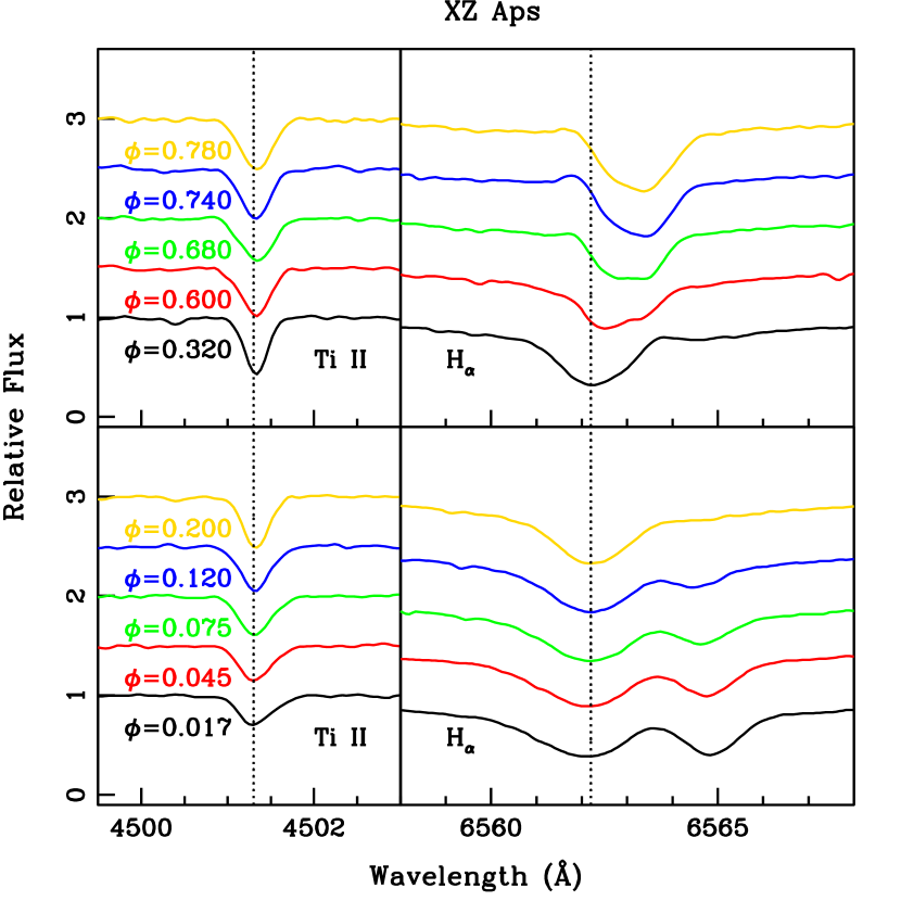
Figure 1: Line profile variations of the XZ Aps combined spectra in the phase range $\phi$ = 0.017–0.78 for a typical metal line, Ti II 4501.3 Å (left-hand panels), and for H$\alpha$ (right-hand panels). The metal line appears to be sharpest near $\phi$ = 0.32. However, the line profile variations are very small from $\phi$ $\approx$ 0.25 to 0.55 (see Figure 3, and so we show only the $\phi$ = 0.32 spectrum here.)

We designated a series of phase bins per star. Using the phase information in Table 4 of FPS11, we selected about 10–15 spectra with similar phases for combining, in order to significantly increase the signal-to-noise for abundance analysis. For a Blazhko star, we treated the cycles of different RV amplitudes separately, which resulted in more than one series of phase bins. Prior to combination, the individual spectra were examined carefully, especially near the H$\alpha$ profile, to guard against any obvious phase contamination in the averaged spectrum. The H$\alpha$ profile was chosen because it varied significantly from phase-to-phase, and thus any anomalies in its appearance could be identified easily. The number of spectra for combining was decided on a case-by-case basis through these inspections of the individual spectra. We have listed/named the single combined spectrum as the mid-point of starting and ending phases (e.g., a spectrum at phase 0.015 is the combination of spectra that have phases from 0 to 0.03). The shapes of metal line profiles of combined XZ Aps and RV Oct spectra and their associated H$\alpha$ line profiles (after correction for scattered light, see below) are displayed in Figure 1–4. The figures show distinctive variations of H$\alpha$ profiles from phase to phase.

Conventional procedures for removal of scattered light from our spectra are not feasible because of the short (4 arcsec) entrance aperture of the du Pont echelle. Therefore, we are obliged to model the scattered light by the procedures described in §3.1 of FPS11. We proceed as described below.

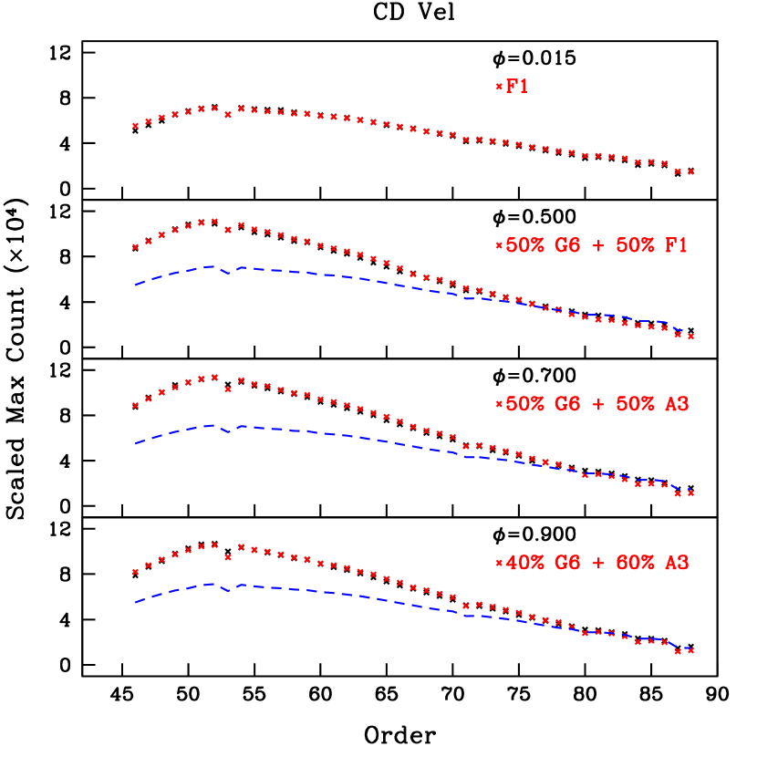
Figure 5: Comparisons between the spectral energy distributions (SEDs) of standard stars and/or family of their spectral combination (red crosses), and the combined spectra of CD Vel in different phases (black crosses). The counts in each order were arbitrarily scaled for comparisons. These comparisons were used to decide the amount of scattered light correction for each order. The blue dashed lines in the bottom three panels are the same and the points in the top panel, thus representing the SED of the pure F1 spectral type for comparison with the “mixed” spectral types.

To correct for scattered light in the RR Lyr spectra, we first measured the peak count of each order of the combined spectrum for each phase. This yielded the relative spectral energy distribution (SED). We did the same for the spectra of standard stars (see FPS11) and for a family of combinations of their spectra (e.g., one such composite contained 50$\%$ of a G6 and 50$\%$ of an A3 spectral type). Subsequently, we compared the SEDs of standard stars and their combination family with the combined RR Lyr spectrum. We illustrate SED comparisons between the spectra of standard stars and their combination family with RR Lyr spectra in different phases in Figure 5.

Once the best match was found (as shown in Figure 5), we normalized the combined spectrum with IRAF’s CONTINUUM task in the ONED package. We then subtracted the corresponding fractional contribution of the inter-order background to the on-order starlight, $b_{\lambda}/s_{\lambda}$ (corrected by a factor of 5/3 due to different aperture extractions, see FPS11), of a particular spectral type from each order. The $b_{\lambda}/s_{\lambda}$ values were listed in Table 3 of FPS11 The RR Lyr spectrum corrected for scattered light was then renormalized and stitched into 4 long wavelength spectra. These 4 long wavelength spectra per phase bin were used for the abundance analysis.

To justify that the scattered light correction method we employed here was reasonable, we obtained a spectrum of the well-studied metal-poor star HD 140283, reduced it and applied the scattered light correction in the same manner as we did for our RR Lyr. Comparing the EWs of Fe I lines in the blue and red wavelength regions (after scattered light correction) with EWs of Aoki et al. (2002), we find: $\Delta$EW(Aoki$-$us)=$-1.3\pm 0.4$ mÅ, $\sigma=2.6$ mÅ, 48 lines, which is good agreement.

4 LINE LIST AND EQUIVALENT WIDTH MEASUREMENTS

We employed the atomic line list compiled by For & Sneden (2010) for our analysis. The line wavelengths, excitation potentials (EP) and oscillator strengths ($\log gf$) and their sources are given in that paper. For each star, we measured the EWs of unblended atomic absorption lines semi-automatically with SPECTRE. Each line measurement was visually inspected prior to acceptance of its EW. Due to the asymmetric line profiles of RR Lyr stars over most of their cycle, we adopted the method of integrating over the relative absorption across a line profile to determine the EW values. Fitting a Gaussian to the line profile was adopted only at the phase with sharp (symmetric), non-distorted absorption lines. We excluded strong lines, defined as those with reduced widths, $\log\rm RW\equiv\log EW/\lambda\gtrsim-4.0$, because they are on the damping portion of the curve-of-growth and thus abundances derived from them are sensitive to multiple line formation factors. Very weak lines ($\log\rm RW$ $<$ $-$5.9) were also excluded because the EW measurement errors were too large.

5 INITIAL MODEL ATMOSPHERE PARAMETERS

We derived abundances in our RR Lyr stars through EW matching and spectrum syntheses. Both methods require model stellar atmospheres that are characterized by parameters effective temperature ($T_{\rm eff}$), surface gravity (log g), metallicity ([M/H]) and microturbulence ($v_{\rm t}$). We constructed the models by interpolating in Kurucz’s non-convective-overshooting atmosphere model grid (Castelli et al., 1997), using software developed by A. McWilliam and I. Ivans. The elemental abundances were subsequently derived using the latest 2010 version local thermodynamic equilibrium (LTE), plane-parallel atmosphere spectral line synthesis code MOOG (Sneden, 1973). This code includes treatment of electron scattering contributions to the near-UV continuum that have been implemented by Sobeck et al. (2011). Details on estimating initial stellar parameters are given in the following subsections.

5.1 Effective Temperature

Use of spectroscopic constraints alone to determine model atmosphere parameters can lead to ambiguous results, due to degeneracies in the responses of individual EWs changes in various quantities. This is especially true for $T_{\rm eff}$ and $v_{\rm t}$: the lines with lower EPs are usually those with larger EWs, making it difficult to simultaneously solve for $T_{\rm eff}$ and $v_{\rm t}$ unambiguously. It is important to have a good initial guess at $T_{\rm eff}$ from other data, and the standard method involves photometric color transformations. Using color-temperature transformations (e.g., Alonso et al., 1996, Ramírez & Meléndez, 2005) it is straightforward to obtain the temperatures of the RR Lyr throughout their pulsational cycles. However, our program stars lack the necessary photometric information. Extensive $V$ magnitude data are available for all our stars at the All-Sky Automated Survey (ASAS) website (Pojmanski, 2002) but $I$ magnitude data have not been gathered. Therefore we do not have any color information for our stars and development of a new, indirect method to estimate initial $T_{\rm eff}$ values for at individual phases of our RR Lyr stars is needed.

5.1.1 Color–Temperature Transformations

Temperature transformations from photometric indices are generally achieved with either a stellar atmosphere model (see Liu & Janes, 1990) or an empirical color–temperature calibration (see Clementini et al., 1995). The latter method can be problematic because it does not account easily for metallicity and surface gravity effects. Of particular importance is the gravity, which varies about a factor of ten during the pulsational cycle of an RRab star. Ideally, hydrodynamical models would be more suitable to describe RR Lyr atmospheres (and thus their $T_{\rm eff}$ values at any phase) but no such models capable of dealing with the fast moving atmospheres of RR Lyr exist yet. Luckily the most dynamical phase (near minimum radius), in which a shock wave is produced during the rapid acceleration of an RR Lyr atmosphere, only occurs in a very short timescale ($\sim 15$ min). Castor (1972) found that a dynamical atmosphere model produces a continuous spectrum that is nearly indistinguishable from that of a hydrostatic atmosphere at the same temperature and gravity in most of the pulsational cycle. A non-linear pulsational model for the prototype star RR Lyr by Kolenberg et al. (2010) shows that the kinetic energy of its atmosphere reaches a minimum at two phases, $\phi$ $\simeq$ 0.35 and 0.90 (see their Figure 1), for which the dynamical effects are small. Accordingly, we assume that the atmospheres of RR Lyrs are in approximate quasi-static equilibrium during most of the pulsational phases.

A mirror-image relation between light and radial velocity variations of Cepheids has been recognized for more than 80 years (Sanford, 1930). Inspection of the extensive data of Liu & Janes (1989, 1990), hereafter LJ89 and LJ90, shows that similar mirror image relations also exist between the color indices and radial velocities of RR Lyrae stars. Because we do not have suitable color data for our RRab stars, we decided to use this mirror-image characteristic to estimate colors of our stars at the phases of our spectroscopic observations. We used the data of Liu & Janes to establish relations between radial velocity and color indices. We then used these relations to estimate colors, and hence temperatures from appropriate color-temperature relations. This procedure works well: radial velocity is a proxy for color index.

We chose eight RRab stars from LJ89 (SW And, RR Cet, SU Dra, RX Eri, RR Leo, TT Lyn, AR Per and TU Uma). For these stars we first extracted $B-V$, $V-R_{c}$ and $V-I_{c}$ color indices and their RVs that correspond to our defined 11 phase bins (e.g., $\phi=$ 0, 0.05, 0.1, 0.2, 0.3, 0.4, 0.5, 0.6, 0.7, 0.8 and 0.85, see Table 3 for details). The color index of a phase that most closely matches one of our phase bins was adopted (e.g., RV at phase 0.8525 in LJ89 was adopted as our RV for the defined phase 0.85). The published color curves were not corrected for the reddening. Thus, we corrected the color indices of $B-V$, $V-R_{c}$ and $V-I_{c}$ as follow:

$$c(colors)=(colors)-E(colors),$$ (1)

where $c(colors)$ is the corrected color index and $E(colors)=kE(B-V)$. The values of $k$ and $E(B-V)$ were adopted from Tables 2 $\&$ 3 of LJ90. We refer the reader to §2b of LJ90 for the extensive discussion of their choice of reddening.

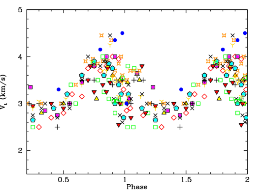
Figure 19: The microturbulence as a function of phase of all of our program stars. The symbols represent the same stars as labeled in Figure 15.

To transform the color indices of LJ89 into $T_{\rm eff}$ values, a set of synthetic colors computed from model stellar atmosphere grids is needed. Calculated colors are given in Table 7 of LJ90, but those are based on relatively old model atmospheres (Kurucz, 1979). Instead, we created grids that correspond to the metallicity of RR Lyr in LJ90 with Kurucz’s non-convective-overshooting atmosphere models (Castelli et al., 1997). A surface gravity of $\log g=3.0$ was chosen initially because it is a better representation for the mean effective gravity (with only small variations) of an RR Lyr star during phases 0–0.8 (i.e., $3.2<\log g<2.8$; see Figure 1 of LJ90). However, the effective gravity (which will be described in detail in §5.2) is an approximation for compensating the dynamical nature of the RR Lyr atmospheres, which could be quite different than the actual surface gravity in the static model that we applied here. Our tests showed that the transformed $T_{\rm eff}$ with $\log g=3.0$ model was persistently too high to fulfill the spectroscopic constraint for all phases of our RR Lyr during the initial spectroscopic analysis. We noted that the effective gravity calculated in LJ89 were based on the Baade-Wesselink (BW) method. For & Sneden (2010) showed that the log g derived from the BW method by others were systematically higher than indicated by the spectroscopic method for non-variable horizontal branch stars analysis (see Figure 19 of For & Sneden, 2010). Therefore, we employed models with $\log g=2.0$; the new grids are presented in Table 2.

The subsequent color–temperature transformation was carried out by employing a linear interpolation scheme:

$$\mbox{$T_{\rm eff}$}=\mbox{$T_{\rm eff}$}_{1}+\frac{(\mbox{$T_{\rm eff}$}_{2}-\mbox{$T_{\rm eff}$}_{1})}{(c_{2}-c_{1})}\times(c_{*}-c_{1}),$$ (2)

where $\mbox{$T_{\rm eff}$}_{1}$ and $\mbox{$T_{\rm eff}$}_{2}$ are two effective temperatures from the grid, c₁ and c₂ are the color indices of $T_{\rm eff}$₁, $T_{\rm eff}$₂, and c_∗ is the color index of the star at a particular phase.

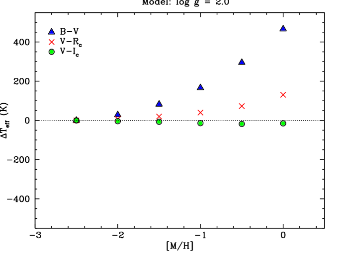
Figure 6: The deviation of effective temperature calculated from different synthetic color indices as a function of metallicity. The color indices are computed at phase 0.3 of RR Cet with a single gravity, log g = 2.0. The temperature difference was taken between the calculated $T_{\rm eff}$ at that particular [M/H] and the $T_{\rm eff}$ at [M/H] = $-$2.5. Symbols represent $T_{\rm eff}$ values derived from these color indices: $B-V$ (triangles); $V-R_{\rm c}$ (crosses); and $V-I_{\rm c}$ (circles).

To derive the $T_{\rm eff}$–phase relations, we employed only the $V-I_{c}$ color because the color–temperature transformation became less sensitive to metallicity and gravity at longer wavelengths. We demonstrate the sensitivity of transformed $T_{\rm eff}$ as a function of metallicity in Figure 6. The strong dependence of $B-V$ on metallicity is caused by the line blanketing in the $B$ filter. The calculated $T_{\rm eff}$ for a given observed color index was adopted at phase 0.3 of RR Cet for different metallicities with fixed log g. The difference was taken between the calculated $T_{\rm eff}$ at that particular [M/H] minus the $T_{\rm eff}$ at [M/H]$=-2.5$.

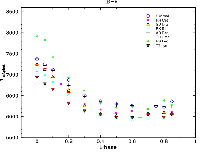
Figure 7: The effective temperatures transformed from $B-V$ color indices as a function of phase. The different symbols represent the 8 RRab variables (SW And, RR Cet, SU Dra, RX Eri, AR Per, TU Uma, RR Leo and TT Lyn) selected from LJ89 and LJ90. They are used as our “calibration stars”.

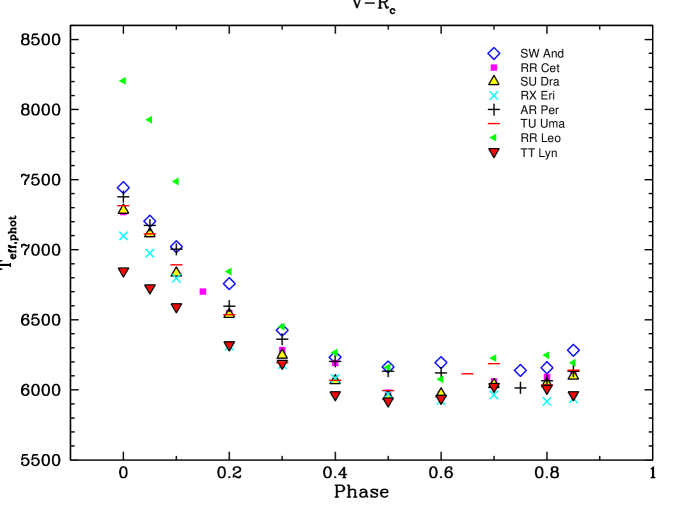
Figure 8: The effective temperatures transformed from $V-R_{\rm c}$ color indices as a function of phase. The different symbols represent the same RRab variables as shown in Figure 7.

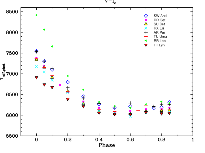
Figure 9: The effective temperatures transformed from $V-R_{\rm c}$ color indices as a function of phase. The different symbols represent the same RRab variables as shown in Figure 7. Individual $V-I_{\rm c}$ vs phase relations are used to fit 4^th-order polynomial curves, which are treated as our “calibration curves”.

We summarize the color–temperature transformations of each phase in Table 3. In Figures 7, 8, and 9 we show the transformed $T_{\rm eff}$ from $B-V$, $V-R_{c}$ and $V-I_{c}$, respectively, versus phase for eight selected RRab variables, which will be called “calibration stars” in the following sections.

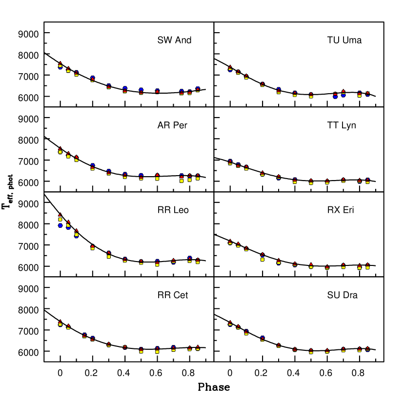
Figure 10: The transformed $T_{\rm eff}$ from different color indices as a function of phase for the selected 8 RRab variables from LJ89 and LJ90. The solid lines are fitted 4^th-order polynomials to the $V-I_{\rm c}$ curves. Symbols refer to $T_{\rm eff}$ values derived from the color indices: $B-V$ (blue hexagons); $V-R_{\rm c}$ (yellow squares) and $V-I_{\rm c}$ (red triangles).

Subsequently, we fitted 4^th-order polynomials to $T_{\rm eff}$ values transformed from $V-I_{c}$ vs phase. The fitted curves are called “calibration curves” for our RR Lyr. Phases during the rising branch of RR Lyr (i.e., after phase $\sim$0.85) were excluded to avoid any artificial fit to the data. We considered the $T_{\rm eff}$ at those phases to be close to their descending branch (i.e., phase 0.9 equivalent to phase 0.1). This assumption is problematic, but we are unaware of a better alternative. The derived 4^th-order polynomial equations are given in Table 4 and Figure 10 shows the fit to the $V-I_{c}$ data.

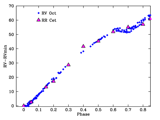
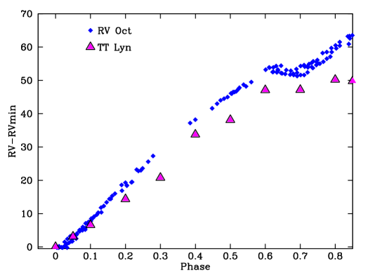
Figure 11: Demonstration of selecting the best calibration curves by comparing the RV$-$RVmin curve of our RV Oct to RV$-$RVmin curves of RR Cet (top panel) and TT Lyn (bottom panel). The top panel shows the best match pulsational behavior. Symbols refer to RV Oct (blue diamonds) and RR Cet $\&$ TT Lyn (magenta triangles).

To decide which “calibration curves” to use for obtaining the initial $T_{\rm eff}$ throughout the pulsational cycle of our RR Lyr, we compared our RV curves to the RV curves of those eight RRab variables selected from LJ89. An example of such comparison is shown in Figure 11, where the RV curve of RV Oct matched the RV curve of RR Cet but not that of TT Lyn. We found that comparing the RV curves of our Blazhko stars to the RV curves of calibration stars was particularly difficult. The RV curves of calibration stars represent typical pulsation RV amplitudes of non-Blazhko RRab variables. In the case of our Blazhko stars, the RV amplitudes vary significantly with Blazhko phase and we could not find any close match between the RV curves of our Blazhko stars and those of our calibration stars. Perforce, we selected the most closely matching RV curve of a calibration star and used its calibration curve to obtain the initial $T_{\rm eff}$ in those cases.

5.2 Surface Gravity

Due to pulsation, the gravity of RR Lyr varies throughout the pulsational cycle. Therefore, the observed gravity at a given phase, which we call the effective gravity, must include a dynamical acceleration term:

$$g_{\rm eff}=\frac{GM}{R^{2}}+\frac{d^{2}R}{dt^{2}},$$ (3)

where $M$ and $R$ are the mass and the radius of the star. The first term represents the mean gravity of the star, which can be derived from its mass and mean radius. The second term represents the variation of gravity, which takes into account the acceleration of the moving atmosphere. It can be determined by differentiating the radial velocity curve.

The mass and mean radius can be derived via the BW method, for which photometric information is required. Since we do not have lightcurves for our RR Lyr stars, we chose a fixed log g = 2.0 as the initial gravity estimate.

5.3 Metallicity and Microturbulence

We adopted the [Fe/H] values of Layden (1994) as listed in Table 1 of Preston (2009) as our initial metallicity estimates. There is no previous derived metallicity for DT Hya and CD Vel in the literature. For these stars we employed [M/H] $=-1.5$, which is similar to the mean [M/H] of our other program stars.

A constant microturbulence is generally assumed throughout the layers of stellar atmospheres. Apart from simplicity, there is no evidence to support this assumption for real stars. In fact, some studies suggested that non-constant microturbulence is more appropriate to physically describe a stellar atmosphere (e.g., see Hardorp & Scholz, 1967; Kolenberg et al., 2010). In addition, the presence of shock waves during the RR Lyr pulsational cycle makes $v_{\rm t}$ unlikely to be constant in their atmospheres (see theoretical work by Fokin et al., 1999a). To perform the spectroscopic analysis, we adopted $v_{\rm t}$ = 3 km s^-1 as an initial guess and set it as a free parameter. The variation of microturbulence as a function of phase/$T_{\rm eff}$ is discussed in the following sections.

6 ADOPTED MODEL ATMOSPHERE PARAMETERS

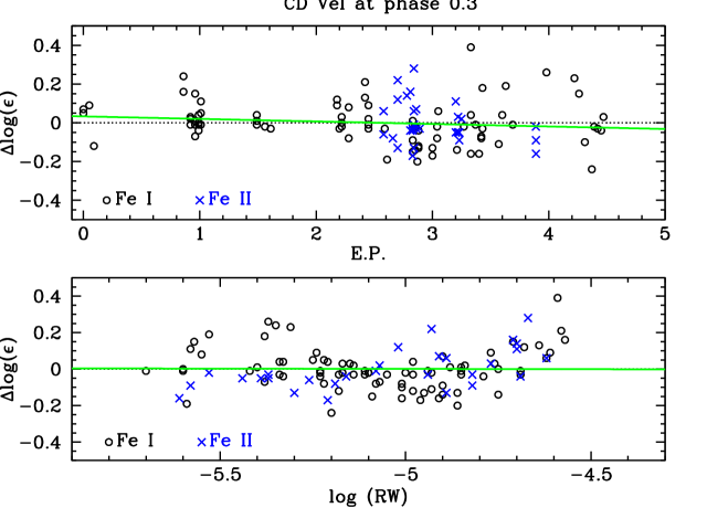
Figure 12: Differences of individual Fe I and Fe II line abundances as functions of EP (top panel) and log RW with the final spectroscopically-constrained model atmosphere parameters of CD Vel at $\phi$ = 0.3. The black open circles and blue crosses represent Fe I and Fe II, respectively, as indicated in the panel legends. The green solid lines show the (negligible) trends of these abundances with EP and log RW for Fe I lines.

Final model atmosphere parameters were determined by iteration through spectroscopic constraints: (1) for $T_{\rm eff}$, that the abundances of individual Fe I and Fe II lines show no trend with EP; (2) for $v_{\rm t}$, that the abundances of individual Fe I and Fe II lines show no trend with reduced width $\log\,(\rm{RW})$; (3) for log g, that ionization equilibrium be achieved by requiring equality between the abundances derived from the Fe I and Fe II species; and (4) for metallicity [M/H], that its value is consistent with the [Fe I/H] determination. An example of fulfilling the spectroscopic constraints is presented in Figure 12. The linear regression lines shown in the figure indicate that $T_{\rm eff}$ and $v_{\rm t}$ have been determined to within the line-scatter uncertainties, and the agreement between the mean abundances for the two Fe species indicates choice of a log g that satisfies the Saha ionization balance.

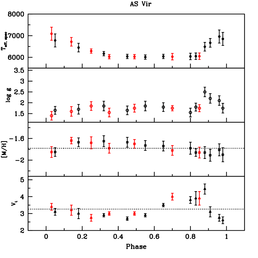
Figure 14: Derived stellar parameters for AS Vir. This figure is similar to Figure 13, except different color symbols represent different cycles being considered for combining the spectra of this Blazhko variable.

We present the derived stellar parameters vs pulsational phase of RV Oct and AS Vir as examples for Blazhko and non-Blazhko effect stars, respectively, in Figures 13 and 14. The dashed lines represent the mean values. The top and second panels show the typical $T_{\rm eff}$ and log g changes in the atmosphere of RR Lyr during the pulsational cycle. The third panel shows the consistency of our derived [M/H]. The bottom panel shows the variation of $v_{\rm t}$ as a function of phase. Interpolated model atmospheres, constructed as described in §5 with the derived parameters listed in Table 5, were used to derive the abundances of each star.

6.1 Parameter Uncertainties

To estimate the effects of uncertainties in our spectroscopically-based $T_{\rm eff}$ values on derived abundances, we varied the derived $T_{\rm eff}$ of RV Oct (as an example) by raising $T_{\rm eff}$ by different amounts for all phases. The uncertainty of $T_{\rm eff}$ was determined for a particular phase when the raised $T_{\rm eff}$ produced a large trend of derived log $\epsilon$(Fe) ($\Delta$ log $\epsilon$(Fe) $>\pm 0.1$) with excitation potential. This yielded estimated $T_{\rm eff}$ errors of 100–300 K throughout the cycle. The largest uncertainties generally were encountered during the most rapidly-changing parts of the pulsational cycles ($\phi<$ 0.3 and $\phi>$ 0.8). The initial $T_{\rm eff}$ values for phase 0.9 onward were assumed to be close to their descending branch (as discussed in §5.1.1), which resulted in larger uncertainty considered that the $T_{\rm eff}$ versus phase curve was asymmetric. In addition, fewer Fe lines are available for EW measurements in the hotter phases of the descending and rising branches than at other (cooler) phases.

We estimated $v_{\rm t}$ uncertainties in a similar manner, assessing the trends of log $\epsilon$(Fe) with $\log\,(\rm{RW})$. This yielded $v_{t}$ errors of 0.1–0.4 km s^-1 throughout the cycle. Finally, assuming that $\log g$ values based on the neutral/ion ionization balance of Fe abundance are correct, then from the dependence of Fe II abundances on $\log g$ we estimated the $\log g$ uncertainty to be $2\sigma$ of the Fe II abundance error. The typical mean error of log g is $\sim 0.2$ dex per star. We adopted the internal error ($\sigma$) of Fe I abundances as the model [M/H] error.

6.2 Reliability of Derived Stellar Parameters

6.2.1 Derived Effective Temperature

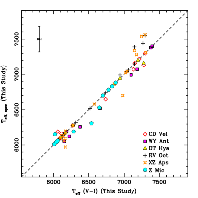
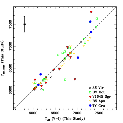
Figure 15: Comparison of derived spectroscopic $T_{\rm eff}$ with photometric $T_{\rm eff}$. The top and bottom panels contain non-Blazhko and Blazhko stars, respectively. Symbols representing individual stars are given in the legends. For the clarity in the figure, we do not plot the error bar for each value, but instead indicate typical uncertainties for $T_{\rm eff}$_,spec and $T_{\rm eff}$_,(V-I).

We compare our final spectroscopic $T_{\rm eff}$’s with the initial values that were derived from the calibration curves, in top and bottom panels of Figure 15 for non-Blazhko and Blazhko stars, respectively. The scatter with respect to the unity line for the non-Blazhko stars is $\Delta$($T_{\rm eff,phot}-T_{\rm eff,spec}$)$~{}=4\pm 10$ K, $\sigma=92$ K, $N=87$, and it is somewhat larger for the Blazhko stars, $\Delta$($T_{\rm eff,phot}-T_{\rm eff,spec}$)$~{}=8\pm 17$ K, $\sigma=151$ K, $N=78$. Most cases of exact agreement (i.e., $\Delta$$T_{\rm eff}$= 0) were artificially caused by the spectroscopic constraints method that we used. Those initial $T_{\rm eff}$ values either yielded no trend or small trend ($\Delta$ log $\epsilon$(Fe) = 0.05) with EP during first iteration. Based on the overall calculated $\Delta$$T_{\rm eff}$, we conclude that even though the RV curves of Blazhko stars might not match the RV curves of calibration stars, the initial $T_{\rm eff}$ values derived from the calibration curves worked reasonably well. We also showed in a previous section that the selected initial $T_{\rm eff}$ yielded consistent stellar parameters throughout the pulsational phase for any cycle in Blazhko stars (see Figure 14 for example).

We made another comparison with the study of TY Gru (Preston et al., 2006b) that was based on MIKE Magellan spectra. Their derived stellar parameters near minimum light for TY Gru were $T_{\rm eff}$ = 6250$\pm$150 K, log g = 2.3$\pm$0.2 dex, [M/H] = $-2.0\pm 0.2$, and $v_{\rm t}$ = 4.1$\pm$0.2 km s^-1. Our derived stellar parameters at phase 0.8 were $T_{\rm eff}$ = 6360$\pm$150 K, log g = 2.05$\pm$0.30 and $v_{\rm t}$ = 4.15$\pm$0.4 km s^-1, which are within the uncertainties of results of Preston et al. (2006b).

6.2.2 Derived Surface Gravity

The log g derived by use of standard spectroscopic constraints, i.e., the ionization balance between neutral and ionized species, may be lower than the trigonometric log g (see e.g., Allende Prieto et al., 1999) if radiative processes act to ionize neutral species beyond standard Saha collisional values. This is a known issue and has been demonstrated with studies of bright metal-poor stars with well-determined distances such as, HD 140283 (as mentioned in §3).

We performed a standard spectroscopic analysis of HD 140283. A summary of the results of this investigation and comparison with other studies is given in Table 6. The spectroscopic log g values derived in Hosford et al. (2009) and Aoki et al. (2002) are lower than those obtained with other methods, and are essentially within errors of our spectroscopic values for HD 140283. We also note that the slightly higher log g determined by Aoki et al. than by either Hosford et al. or us is due to their use of Ti lines, which has been shown to cause a systematic offset in spectroscopic derived log g (see §5.3 of For & Sneden, 2010).

Ideally we should compare the derived spectroscopic log g with physical or trigonometric log g that can be derived from stellar parallaxes. However, this is not possible for our our RR Lyr stars, because either the reported parallaxes have large errors, or no parallax data are available. Nevertheless, we may evaluate the physical log g by making assumptions for the following equation:

$$\mbox{log~{}{\it g}}=\log(M/\mbox{$M_{\odot}$})+4\log(T_{\rm eff,spec})-\log(L/L_{\sun})-10.607,$$ (4)

in which the constant was calculated by using the solar $T_{\rm eff}$ and log g values, $M=0.68$ $M_{\odot}$ as typical mass of an HB star and absolute magnitude of $M_{V}=+0.6$ (Castellani et al., 2005), a value consistent with typical RR Lyr stars (Beers et al., 1992). We note that the absolute magnitude is metallicity-dependent, in that a lower metallicity would result in brighter absolute magnitude (see e.g., Gratton, 1998).

Comparing our derived log g values throughout the pulsational cycles with calculated physical log g values, we found that they are systematically lower, $\Delta$log g(calculated$-$us) $=0.80\pm 0.02$ dex, $\sigma=0.28$ dex, $N=165$. The large deviation is partly related to the assumptions we have made for stellar mass, absolute magnitude, and treatment of gravity as mean gravity instead of effective gravity (as described in § 5.2). Significant departures from LTE in the ionization equilibrium also could drive our spectroscopic gravities to artificially low values. For example, see the discussion by Lambert et al. (1996) for NLTE effects on Fe I and Fe II lines in RR Lyr. However, Clementini et al. (1995) argue that NLTE effects are small in these kinds of stars. Resolution of the NLTE question is beyond the scope of our study, but we urge further work on this point in the future.

Finally, note that despite the lower derived log g values for our RR Lyr throughout their pulsational cycles, the trend of our derived log g variation (see e.g., Figure 13) is quite similar to the effective gravity variation as shown in Figure 1 of LJ90.

6.2.3 Derived Metallicity

The metallicities of RR Lyr are commonly derived from $\Delta S$–[Fe/H] relations calibrated by abundances derived from high-resolution spectroscopy. The initial investigation in this area was made by Preston (1961b), who employed the single-layer-atmosphere differential abundance formalism of Greenstein (1948) and Aller (1953), with line identifications taken from Swensson (1946) and Greenstein (1947). This calibration was supplanted by subsequent analyses of many more RR Lyr by Butler (1975), who also used Greenstein’s method, and by Butler et al. (1982). Layden (1994) adopted the latter of these, now 30 years old, to establish his widely-used abundance scale for the RR Lyr.

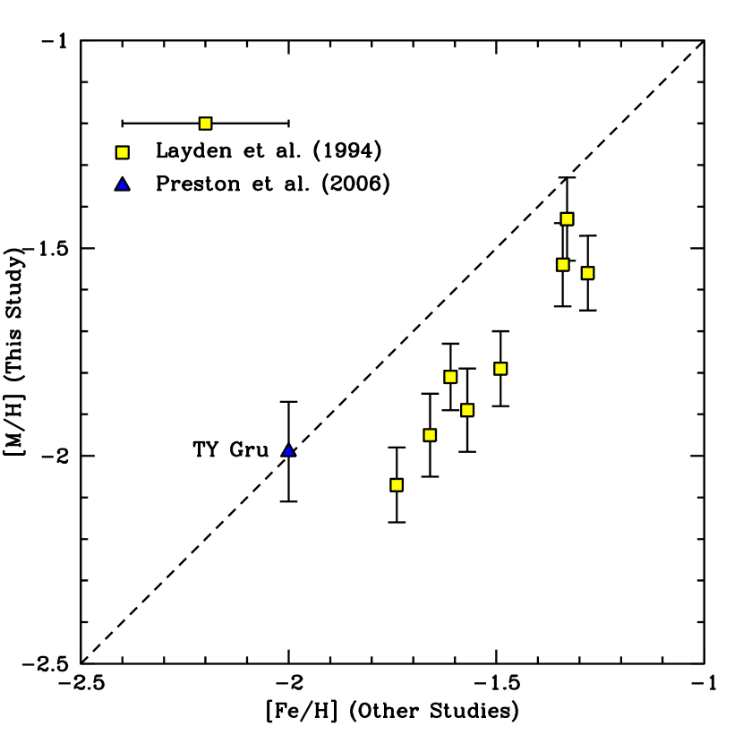
Figure 16: Comparison of derived [M/H] with [Fe/H] of other studies. The symbols represent the values derived from the from the $\Delta S$–metallicity relation by Layden (1994) (yellow squares) and from the spectroscopic method by Preston et al. (2006b) (single blue triangle). For clarity in the figure, we do not plot error bars for each star, but instead indicate typical uncertainties of 0.2 dex for the Layden (1994) paper.

We may compare our derived metallicities with those in Layden (1994). As shown in Figure 16, our [Fe/H] values are lower by $\sim$0.25 dex than those derived by Layden, who used the Butler et al. (1982) results. The downward shift arises from differences in measured equivalent widths, adopted $\log gf$ values, and the use of modern model atmospheres and spectrum analysis codes instead of one-layer curve-of-growth analysis, universally abandoned long ago. We note, finally, that our Fe abundance for TY Gruis is in good accord with that derived from Magellan/MIKE spectra (Preston et al., 2006b).

To further investigate the Fe abundance offset, we refer back to the well-studied subgiant HD 140283, for which our EWs of Fe lines are in good agreement with Aoki et al. (2002). In §3 we used this EW agreement to argue that our scattered light corrections are reasonable. Now using the Aoki et al. measured EWs, their chosen $\log gf$ for Fe I and Fe II lines, and their adopted stellar parameters, we reproduce almost exactly their published log $\epsilon$(Fe) with our analysis code. Then performing an independent atmospheric analysis in the manner employed for our RR Lyr spectra, using Aoki’s data set, we derive $T_{\rm eff}$ about 150 K lower than theirs, which in turn yields in a slightly lower Fe abundance ($\Delta\sim-0.15$ dex). However, a derived $T_{\rm eff}$ for HD 140283 via the photometric “infrared flux method” calibration (Ramírez & Meléndez, 2005) is consistent with our derived spectroscopic $T_{\rm eff}$. This lends indirect support to our general metallicity scale. In addition, we performed a similar test using RR Cet data from Clementini et al. (1995). Adopting their stellar parameters resulted in log $\epsilon$(Fe I) = 5.98 and log $\epsilon$(Fe II) = 6.05. Clementini et al. derived log $\epsilon$(Fe)= 6.18 ($\sigma$ =0.16) and 6.13 ($\sigma$ =0.06) for Fe I and Fe II, respectively. Again, our [Fe/H] value is somewhat less than theirs, but the uncertainties in especially the Fe I abundance are large. We do not intend to solve the absolute scale of metallicity in this paper. Future effort on this issue will be investigated with a wider range of metallicity for the RR Lyr sample. For now, we tentatively recommend a $-0.25$ dex shift to the Layden abundance scale for RR Lyr stars. This downward revision is in accord with recent investigations of the Fe II metallicity scale for the globular clusters (Kraft & Ivans, 2003) and the metal-poor horizontal branch stars of the Galactic field (Preston et al., 2006a; For & Sneden, 2010).

6.3 Microturbulence vs Effective Temperature

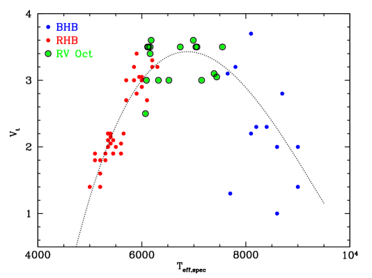
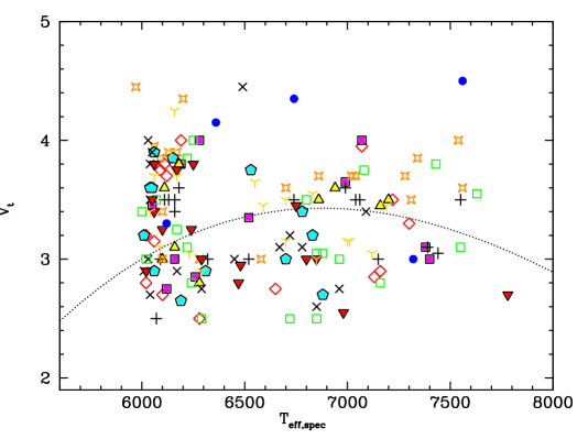
Figure 17: The microturbulence as a function of $T_{\rm eff}$. The top panel shows $v_{\rm t}$ and $T_{\rm eff}$ of RV Oct on the $v_{\rm t}$-$T_{\rm eff}$ plane, with additional data of RHB and BHB stars from For & Sneden (2010). The dashed curve shows a continuous $v_{\rm t}$–$T_{\rm eff}$ relation across the HB. The bottom panel shows all the $v_{\rm t}$ and $T_{\rm eff}$ of all of our program stars on the $v_{\rm t}$-$T_{\rm eff}$ plane near the instability strip region. The symbols represent the same stars as labeled in Figure 15.

We revisit the variation of $v_{\rm t}$ with $T_{\rm eff}$ along the horizontal branch suggested in Figure 7 of For & Sneden (2010). The variation within the instability strip was uncertain in that paper, because the data for RR Lyr came from heterogeneous sources. Now with internally consistent data and analyses we can investigate the variation across the instability strip with more confidence. In the top panel of Figure 17 we show one example by plotting the individual $v_{\rm t}$ values for the stable pulsator RV Oct (Table 5) in the $v_{\rm t}$–$T_{\rm eff}$ diagram of For & Sneden (2010). Excluding one point that is much lower than the rest, the $v_{\rm t}$ values for RV Oct all lie in a relatively narrow range: 3.0 $<$ $v_{\rm t}$ $<$ 3.6 km s^-1. A continuous $v_{\rm t}$-$T_{\rm eff}$ relation across the horizontal branch is suggested, which we interpret empirically by drawing a smooth curve to represent the data points.

When data for all of the RR Lyr in our program are plotted in the bottom panel of Figure 17 we see that the microturbulence values encompass a larger range than do those of RV Oct: 2.5 $<$ $v_{\rm t}$ $<$ 4.5 km s^-1. However, closer inspection of the individual points reveals that the most extreme microturbulence excursions occur in the Blazhko variables. Five out of seven stars with $v_{\rm t}$ $>$ 4.0 km s^-1 are Blazhko stars, as are five out of six stars with $v_{\rm t}$ $<$ 2.6 km s^-1. Thus for most RRab stars in all phases $<$$v_{\rm t}$ $>\sim$ 3.4 km s^-1, with maximum excursions of $\pm$0.6 km s^-1 The range of $v_{\rm t}$ values for our RR Lyr is superficially similar to those reported by Clementini et al. (1995) and Lambert et al. (1996). Evidently $v_{\rm t}$ goes through a maximum in the RR Lyr instability strip of the halo field horizontal branch. The range in $v_{\rm t}$ for each RR Lyr is real, produced by systematic variation during pulsation cycles as we discuss in the next section.

6.4 Microturbulence vs Phase

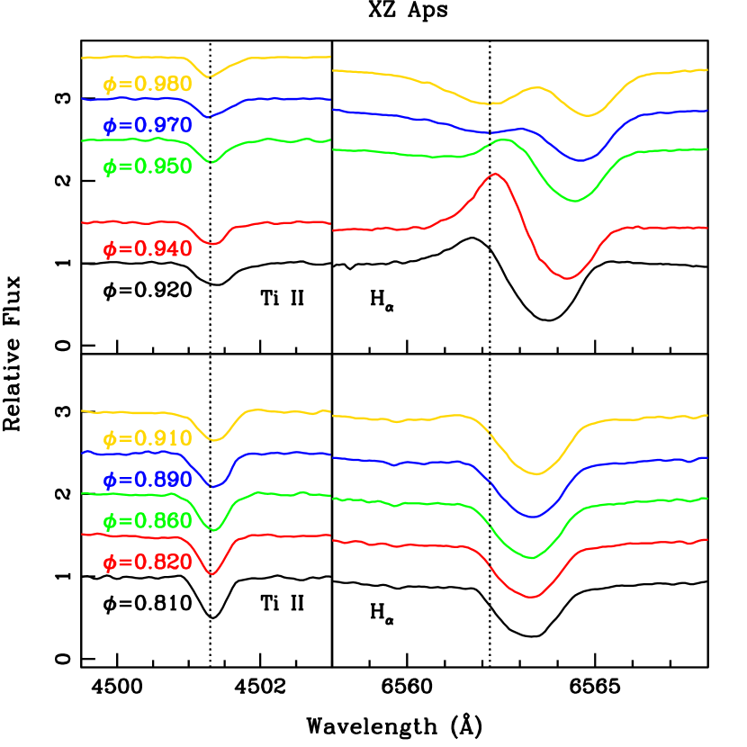
Figure 2: Continuation of the Figure 1 XZ Aps line profile variations for $\phi$ = 0.81–0.98, the rising-light phases of rapid variability in RR Lyr. The H$\alpha$ emission occurs at its highest near $\phi$ = 0.94.

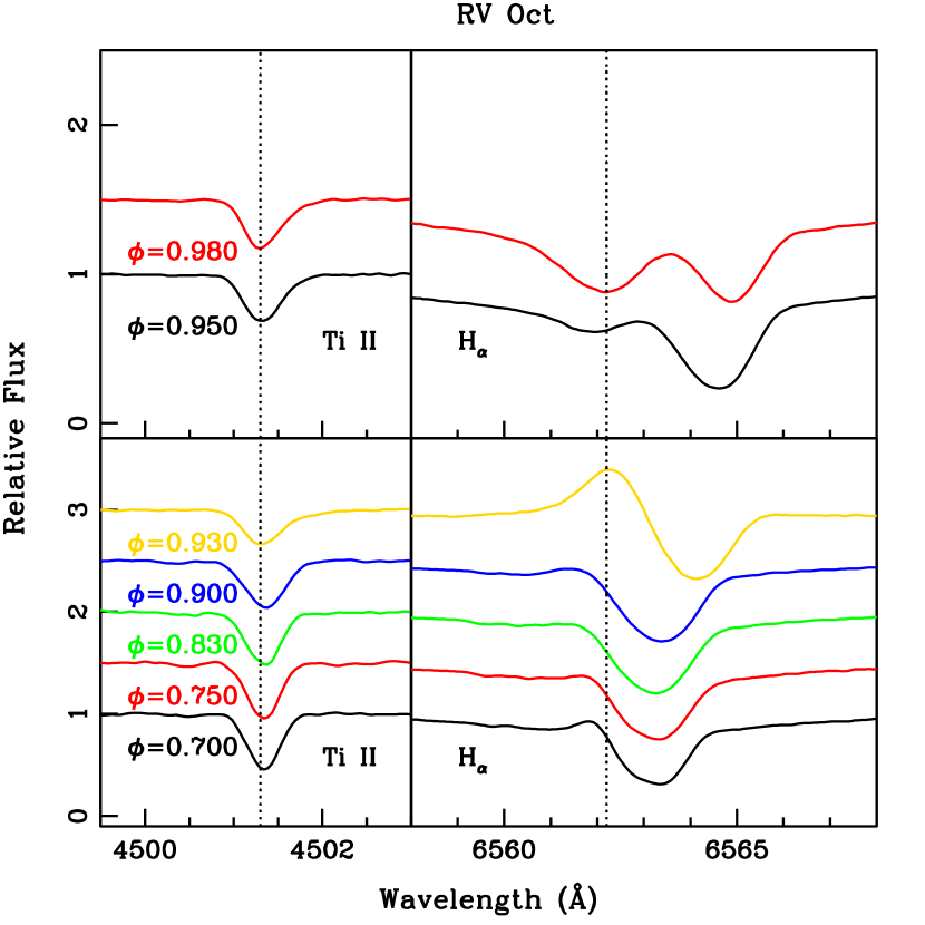
Figure 4: Continuation of Figure 3 for the RV Oct line profile variations in the rapidly changing phase interval from $\phi=$0.7–0.98. The H$\alpha$ emission occurs at its highest near $\phi$ = 0.93.

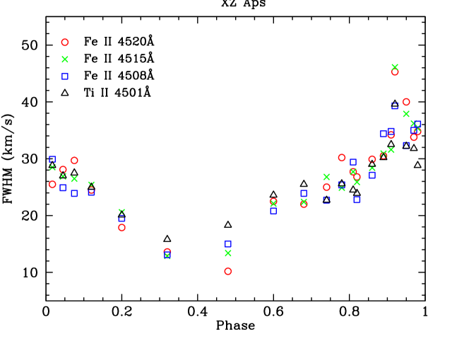
Figure 18: The full width half maximum (FWHM) in km s^-1 of four metal lines of XZ Aps throughout its pulsational cycle. The values have been corrected for instrumental broadening of 11 km s^-1. The FWHM appears to be lowest near $\phi$ $\approx$ 0.3 and has a peak near $\phi$ $\approx$ 0.9, probably associated with the appearance of a shock wave in the photosphere.

Turbulent velocity variations occur during the pulsation cycles of RR Lyraes, as indicated by the investigation of Fokin et al. (1999b), Fokin & Gillet (1997) and Fokin et al. (1999b). The conclusions of these investigators are based on measured FWHM values of metallic lines profiles. These FWHM reach a minimum value briefly near phase 0.35 and then rise to a broad maximum on 0.6 $<$ $\phi$ $<$ 1.2 when two shocks occur above the photosphere. The FWHM that accompany these phenomena exceed our maximum $v_{\rm t}$ values ($<$ 5 km s^-1) at all phases. This is illustrated in Figure 18, where we plot the observed values of FWHM corrected for instrumental broadening of 11 km s^-1 in quadrature term versus phase in the pulsation cycle of XZ Aps. One of these lines, Ti II 4501.3 Å, was the featured metal line of Figures 1 and 2, and the variations in its line width could be seen easily by inspection. Compare our FWHM with those in Figure 6 of Chadid & Gillet (1996) and in Figure 4 of Kolenberg et al. (2010). This broadening of line profiles is a manifestation of macroturbulence, i.e., the bulk motions of gas volumes with dimensions comparable to the thickness of the metallic line-forming regions of the atmosphere.

In our study, we derive values of microturbulence, $v_{\rm t}$, by demanding that the abundances of individual Fe I and Fe II lines show no trend with reduced width $\log$ RW. Our $v_{\rm t}$ are empirical descriptors of motions on length scales small compared to the line-forming region of the atmosphere that broaden the metallic line absorption coefficients and thus intensify line strengths. A plot of our $v_{\rm t}$ values versus phase for all of our RR Lyr is shown in Figure 19. The values of vt and FWHM, derived from independent considerations rise and fall together, indicating that our RR Lyr display growth and decay of turbulent velocities on two length scales together at all phases of their pulsation cycles.

7 The OPTIMAL PHASES

In this section, we discuss the optimal phases for chemical abundances analysis.

The zero point of RR Lyr phase is generally chosen to coincide with the moment of maximum light. Expansion of the atmosphere decelerates from this phase until the layers near the photosphere come to rest near phase $\phi$ $\sim$ 0.35. The expansion is not homologous; see the middle panels of Figure 2 of Fokin & Gillet (1997) and the measured radial velocities of Balmer lines H$\alpha$, H$\beta$ and H$\gamma$ (Preston, 2011). Near $\phi$ $\sim$ 0.35 the atmospheric turbulence is at a relative minimum. Spectra at this phase regime are accordingly best suited for chemical composition analysis because atomic lines suffer minimal blending. This most clearly evident from examination of line widths plotted in Figure 18.

During the optimal $\phi$ $\sim$ 0.35 phase, the effective temperatures of RR Lyr are similar to those of warmer RHB stars (6500 K $<$ $T_{\rm eff}$ $<$ 6000 K). We see many metal lines in the spectra at these temperatures, which make these phases ideal for abundances analyses. Additionally, the sharpness of the line spectra at this phase makes it best for performing spectrum synthesis calculations of complex blended features.

The line smearing and line asymmetry at other phases degrade their value for analysis by spectrum synthesis. Nevertheless, we did not exclude the other phases in our study. In fact, the descending and rising branches of RR Lyr variations have their own advantages. In the post-maximum phase interval ($\phi$ = 0.05–0.15) effective temperatures are similar to cooler BHB stars (7400 K $<$ $T_{\rm eff}$ $<$ 6200 K). Some low EP metal lines that are saturated at cooler phase temperatures are weaker in the hotter parts of RR Lyr cycles, and thus can be more useful in abundance analyses. Thus, we conclude that abundance analysis can be pursued profitably throughout most phases of the pulsation cycles of the RR Lyr.

8 CHEMICAL ABUNDANCES

Metal-poor stars usually have chemical compositions that are enriched in the $\alpha$-elements (e.g., Mg, Si, S, Ca and possibly Ti), i.e., [$\alpha$/Fe] $>$ 0. The $\alpha$-rich behavior is attributed to the presumed predominance of short-lived massive stars that resulted in core collapse Type II supernovae (SNe II) in early Galactic times. The SN explosions contributed large amounts of light $\alpha$-elements (e.g., O, Ne, Mg and Si), lesser amounts of heavier $\alpha$-elements (e.g., Ca and Ti) and even smaller amounts of Fe-peak elements to the ISM (Woosley & Weaver, 1995). The detonation of neutron-rich cores also is supposed to produce heavy $n$-capture isotopes through rapid neutron-capture (hereafter, $n$-capture) nucleosynthesis ($r$-process) where synthesis occurs faster than the $\beta$-decay. As time progressed, longer-lived, lower-mass stars begin to contribute their ejecta by adding more Fe-peak elements through type Ia supernovae (SNe Ia) which exploded, perhaps due to thermonuclear runaway process of accreting binary stars. The asymptotic giant branch (AGB) stellar winds contributed isotopes for slow $n$-capture nucleosynthesis ($s$-process) at later Galactic times. Eventually large amounts of iron polluted the ISM and lowered the $\alpha$/Fe at higher metallicity, i.e. [Fe/H] $\simeq-1$.

Do the abundances of metal-poor RR Lyr conform to this general Pop II chemical composition picture? Using model atmospheres derived as described in §6 (listed in Table 5), we computed chemical abundances for 22 species of 19 elements in $\sim$165 total phase bins for our 11 program stars. Abundances of most elements were derived from EW measurements, by adjusting abundances so that calculated EWs match observed EWs and averaging over all lines of each species. In the cases of Mn I, Sr II, Zr II, Ba II, La II, and Eu II, we employed spectrum syntheses to handle the blending, or hyperfine and/or isotopic substructure present in these lines. We computed theoretical spectra for a variety of assumed abundances for each line, then the assumed abundances were changed iteratively until the theoretical spectra match the observed ones. Syntheses were performed only at phase $\phi$ $\sim$ 0.35 (the optimal phase) of each star except for TY Gru, in which the spectrum at $\phi$ = 0.46 was used. We made this exception because it was the best available phase for spectrum syntheses and for the purpose of cleanly comparing our new abundance results with those of Preston et al. (2006b). We caution that metal line profile distortions are slightly larger at this part of an RR Lyr cycle than at the optimal phase, and therefore larger uncertainties in the derived abundances can be expected.

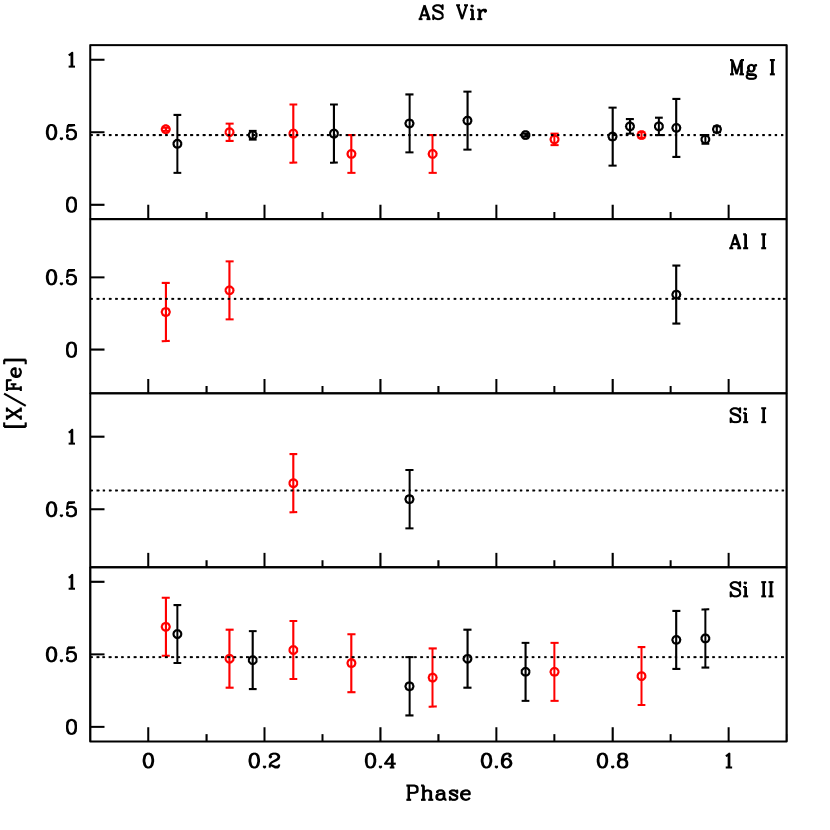
Figure 24: Abundance ratios, [X/Fe], of Mg I, Al I, Si I and Si II as a function of phase for a Blazhko effect star, AS Vir. The dashed lines and color symbols represent the mean values and different cycles being considered for combining the spectra, respectively. The [X/Fe] values are generally consistent throughout the pulsational cycle. The trend in [Si II/Fe] is discussed in § 8.2. NLTE corrections applied to Al and Si abundances whenever appropriate.

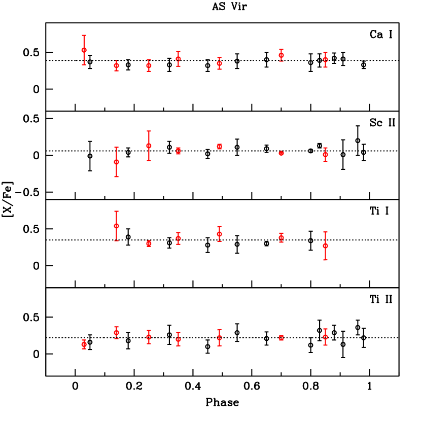
Figure 25: Same as Figure 24, now for Ca I, Sc II, Ti I and Ti II.

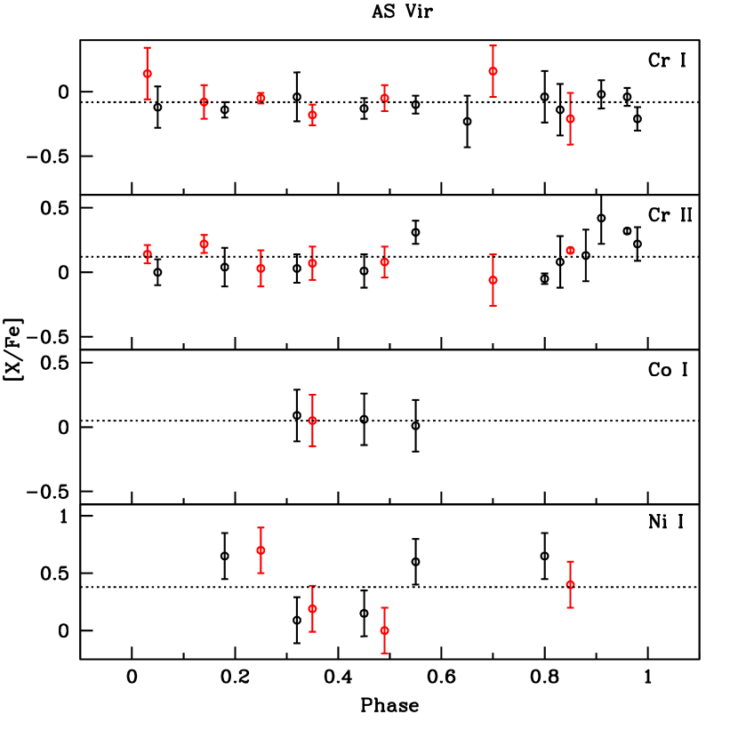
Figure 26: Same as Figure 24, now for Cr I, Cr II, Co I and Ni I. The large phase-to-phase scatter of [Ni I/Fe] is due to the large uncertainties in the derived values.

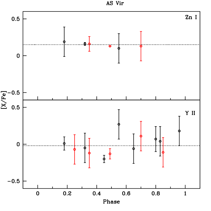
Figure 27: Same as Figure 24, now for Zn I, Y II.

We show relative abundance ratios, [X/Fe], of various elements as a function of phase in Figures 20–23 for RV Oct, a non-Blazhko star; and Figures 24–27 for AS Vir, a Blazhko star. In the case of a Blazhko star, we used different colors to represent different series of phase bins (see discussion in §3). Abundances derived via spectrum synthesis are not presented as a function of phase because they were derived with only one phase as mentioned above. The error bars represent the internal error (line-to-line scatter). We adopted internal error of 0.2 dex for abundances derived from a single line (for plots only). The mean relative abundance ratios are represented by the dashed lines. NLTE corrections were applied to Na, Al and Si abundances whenever appropriate in all figures and tables. Examining these figures, we conclude that the abundances are consistent throughout the pulsational cycles in both Blazhko and non-Blazhko stars.

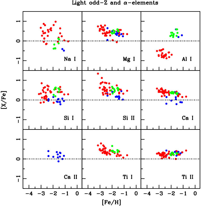
Figure 28: Abundance ratios of light odd-Z and $\alpha$-elements as a function of metallicity. NLTE corrections applied to Na I, Al I, Si I and Si II whenever appropriate. The red and blue dots represent RHB and BHB stars from For & Sneden (2010). The green dots represent the mean abundance ratios of each RR Lyr in our program.

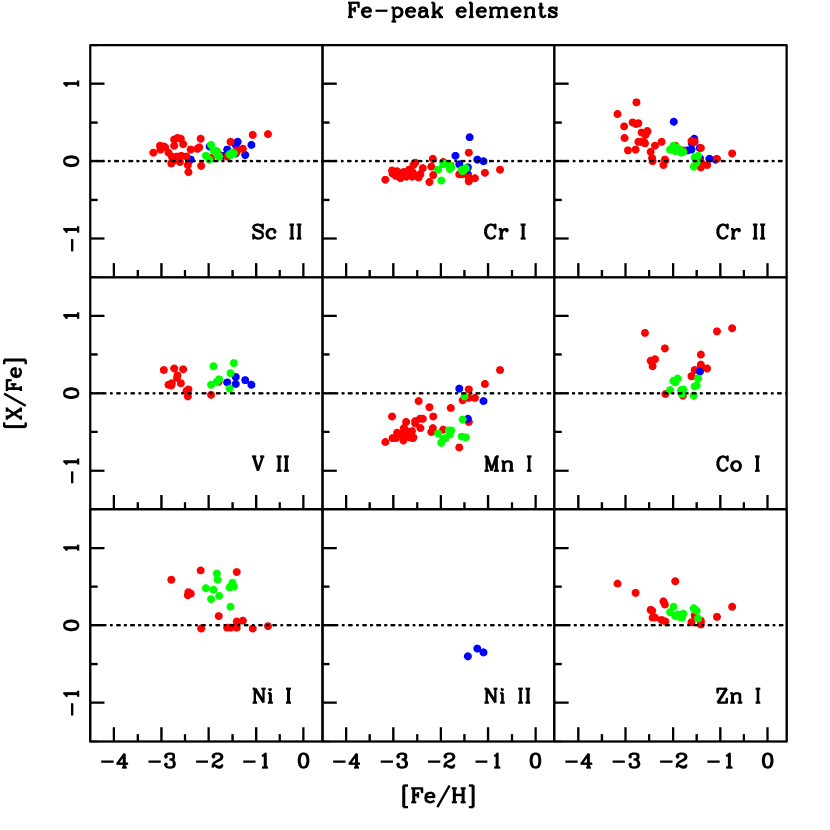
Figure 29: Abundance ratios of Fe-peak elements as a function of metallicity. The red and blue dots represent RHB and BHB stars from For & Sneden (2010). The green dots represent the mean abundance ratios of each RR Lyr in our program.

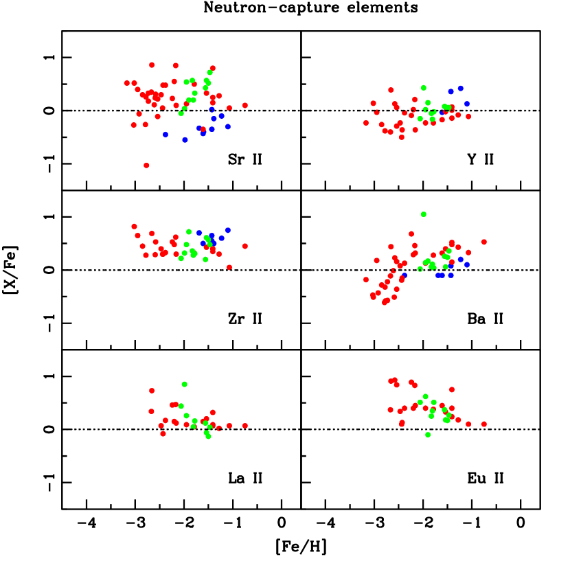
Figure 30: Abundance ratios of $n$-capture elements as a function of metallicity. The red and blue dots represent RHB and BHB stars from For & Sneden (2010). The green dots represent the mean abundance ratios of each RR Lyr in our program.

Tables 7–10 give the derived [X/Fe] of each phase for all program stars. The mean [X/Fe] values of each species for each RRab variable star (green dots) are presented as a function of metallicity in Figures 28–30. We overplot them with the results of RHB (red dots) and BHB (blue dots) stars presented in For & Sneden (2010). We summarize the mean [X/Fe] values of individual RR Lyr in Table 11 and mean [X/Fe] values among different HB groups in Table 12. In the following subsections we comment on individual elements along with the results of RHB and BHB stars from For & Sneden (2010).

8.1 Magnesium, Calcium and Titanium

As mentioned above, metal-poor stars are generally overabundant in $\alpha$-elements. For & Sneden (2010) showed that metal-poor non-variable HB stars possess standard enhancement in these elements. The scatter of our derived light $\alpha$-elements abundances is small for our RRab stars over the whole metallicity range (see Figure 28). We calculated $<$[Mg I/Fe]$>$ $\simeq$ $+$0.48 for RRab stars, which is consistent with the typical $\alpha$-enhancement in field metal-poor stars within that metallicity range.

An offset of [Ca I/Fe] between RHB and BHB stars, $\sim 0.3$ dex, was reported by For & Sneden (2010). Our derived [Ca I/Fe] values are consistent throughout the cycles, both in Blazhko and non-Blazhko stars (see Figures 21 and 25). The mean [Ca/Fe] ratios of our RR Lyr stars also are consistent with those of RHB stars, as shown in Figure 28. We cannot identify the cause of the lower [Ca/Fe] values in the BHB sample and note that we have [Ca I/Fe] values of RRab stars covering all pulsational phases, including those that overlap with the coolest $T_{\rm eff}$ range of some BHB stars ($\sim 7400$ K). We also note that the reported trend of decreasing [Ca/Fe] with increasing $T_{\rm eff}$ for BHB stars as shown in Figure 11 of For & Sneden (2010) does not extend into the RR Lyr domain investigated here.

There are no Ti I lines detectable in the hottest phases of RRab stars, i.e., during those early and late phases of a cycle when $T_{\rm eff}$ overlap with the coolest $T_{\rm eff}$ of the BHB stars ($T_{\rm eff}$$\sim$7400). Thus, the $<$[Ti I/Fe]$>$ values of our program stars as shown here (Figure 28) cover a similar $T_{\rm eff}$ range as the warmer RHB stars. The overall [Ti II/Fe] ratios appear to be constant with [Fe/H], in contrast to the increasing [X/Fe] of the other $\alpha$-elements as metallicity declines. However, if we only consider abundances of Ti I and Ti II derived for RRab stars, we find that both exhibit a flat distribution with a relatively small scatter in this metallicity range (excluding the deviant [Ti I/Fe] of TY Gru). We also find no trend of [Ti I/Fe] with increasing $T_{\rm eff}$ (see e.g., Figure 25 of AS Vir) in contrast to the previous conclusion of For & Sneden (2010) and findings by others (see Lai et al., 2008 and references therein). Investigation of larger sample of RRab stars covering a wider metallicity range is needed to further explore the Ti abundance questions, but the basic result is clear: Ti is overabundant in RRab stars at about the same level as it is in metal-poor stars of other evolutionary states.

8.2 The Alpha Element Silicon: Revisiting A Special Case

Standard LTE abundance analyses find a significant dependence of [Si I/Fe] with temperature in metal-poor field stars (e.g, Cayrel et al., 2004, Cohen et al., 2004, Preston et al., 2006a, Sneden & Lawler, 2008, and Lai et al., 2008). The effect seems to depend solely on $T_{\rm eff}$; no trend with log g has been detected so far. To investigate this issue, Shi et al. (2009) performed an analysis of NLTE effects in Si I in warm metal-poor stars ($T_{\rm eff}$$\geq$ 6000 K). They concluded that the NLTE effects differ from line-to-line and are substantially larger in the lower-excitation blue spectral region transitions ($\chi$ = 1.9 eV; 3905 Å and 4102 Å) than in the higher-excitation red spectral region ($\chi$ $\geq$ 5 eV; e.g., 5690 Å and 6155 Å). Departure from NLTE in warm metal-poor stars is also expected for the Si II 6347 Å and 6371 Å lines.

We revisit the issue of $T_{\rm eff}$ dependence on Si lines with our RRab stars, because the HB samples cover a large temperature range. The [Si I/Fe] values of our program stars were derived either solely from the 3905 Å line or lines in red spectral region throughout the cycle; the selection of lines depended on the $T_{\rm eff}$. To avoid possible blending of the 3905 Å line with a weak CH transition Cohen et al. (2004), which is present in cool stars, we only employed the 3905 Å line during the early or late phases of a pulsational cycle when $T_{\rm eff}$ is similar to the BHB stars ($T_{\rm eff}$ $\geq$ 7400 K).

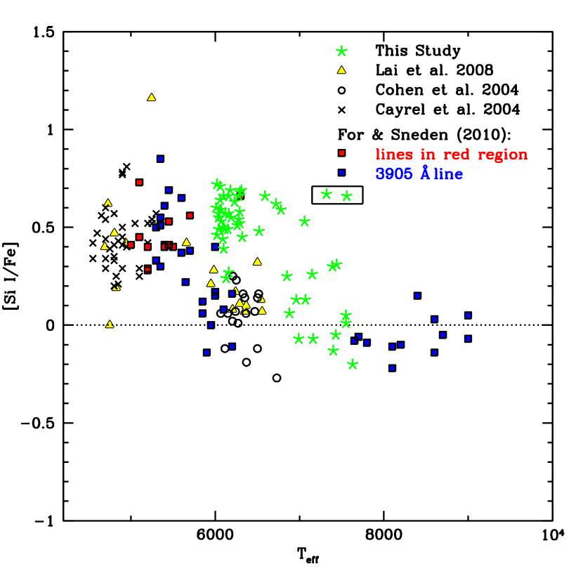
Figure 31: Abundance ratios of [Si I/Fe] of all our program stars in all phases (green stars) vs. spectroscopic $T_{\rm eff}$ , with additional data from Cayrel et al. (2004) (crosses), Cohen et al. (2004) (open circles), Lai et al. (2008) (yellow triangles), and For & Sneden (2010) (blue and red squares). The box marks the two outliers. NLTE correction applied to [Si I/Fe] whenever appropriate.

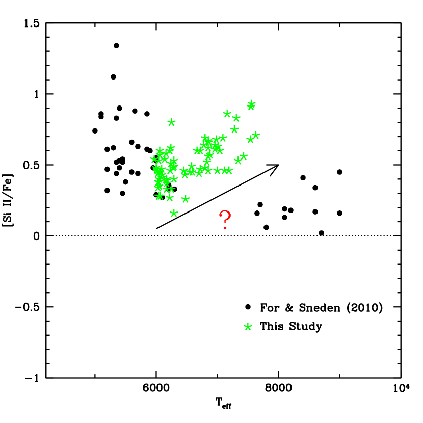
Figure 32: Abundance ratios of [Si II/Fe] of all our program stars in all phases (green stars) vs. spectroscopic $T_{\rm eff}$. NLTE correction applied to [Si II/Fe] whenever appropriate. The black dots denote abundances for the BHB and RHB stars from For & Sneden (2010). A possible increasing [Si II/Fe] trend as a function of increasing $T_{\rm eff}$ is schematically represented in this figure by an arrow, and is discussed in § 8.2.

As shown in Figure 21, the trend of [Si II/Fe] vs phase resembles a similar “shape” as the $T_{\rm eff}$ vs phase plot in the top panel of Figure 13, which suggests a dependence on $T_{\rm eff}$. However, there is no such trend visible in the case of [Si I/Fe] between phase 0–0.8 for RV Oct (see Figure 20). Instead, we detect a significant decline of [Si I/Fe] with increasing $T_{\rm eff}$ for $\phi$ $\gtrsim$ 0.8 in this star. To investigate if NLTE effects could be the cause of such trend, we applied the suggested NLTE corrections of +0.1 dex and $-$0.1 dex by Shi et al. (2009) to the Si I and Si II abundances derived from 3905Å, 6347Å and 6371Å lines. In Figures 31 and 32, we extend For $\&$ Sneden’s Figures 14 and 15 by adding all measured [Si I/Fe] and [Si II/Fe] values that had been corrected for NLTE effects, whenever appropriate. While the scatter of [Si I/Fe] is large for our program stars, we find a possible declining trend with increasing $T_{\rm eff}$ if the two outliers (indicated with a black box in the figure) are ignored. In contrast, the [Si II/Fe] values tend to increase with increasing $T_{\rm eff}$ (as indicated by the arrow in Figure 32). However, we caution the reader that most [Si II/Fe] values were derived with 1–2 lines, for which we anticipate errors of $\pm 0.2$ dex.

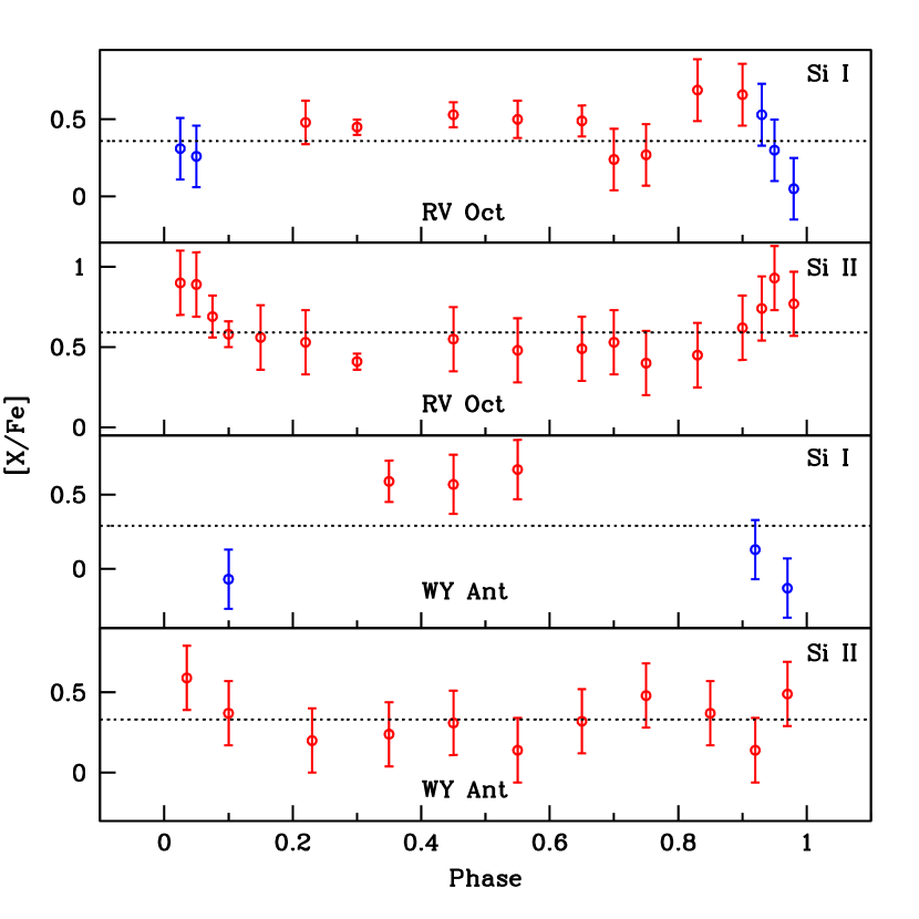
Figure 33: Silicon abundance ratios as a function of phase for RV Oct (first and second panels) and WY Ant (third and forth panels). The blue and red open circles represent the silicon abundances derived from blue and red spectral regions, respectively. NLTE corrections have been applied to the values represented by the blue open circles for [Si I/Fe] and red open circles for [Si II/Fe].

To further investigate the NLTE effects on the trends, we present the silicon abundances as a function of phase for RV Oct and WY Ant in Figure 33, where the blue and red dots represent lines in the blue and red spectral regions, respectively. To emphasize, all values of [Si II/Fe] and only the blue dots of [Si I/Fe] have been corrected for NLTE effects. We find that the NLTE corrections do not resolve the puzzle of $T_{\rm eff}$ dependency in silicon abundances. In fact, even lower [Si I/Fe] values (as seen in the obvious case of WY Ant) were obtained from the use of 3905 Å line in warm metal-poor RRab stars. This suggests that the NLTE computations need to be re-done. A discussion about the line transitions of blue and red spectral lines of Si I is given in Sneden & Lawler (2008). An alternative explanation for the declining and the increasing trends of silicon abundances between phase 0.8–1.0 is that the neutral lines partially disappear during these phases due to the shock wave. This phenomenon was first observed in the spectra of S Arae by Chadid et al. (2008), which the disappearance of Ti I and Fe I lines was shown in their Figure 6. If this is the case, we might expect to see similar effects in other neutral species. We do not see this phenomenon in our data set, and the resolution of this issue is unsatisfactory.

The overall silicon abundances of RRab stars exhibit a large star-to-star scatter, which is similar to the results of RHB and BHB stars (see Figure 28). However, the mean Si abundances, $<$[Si I/Fe]$>$ = +0.48 and $<$[Si II/Fe]$>$ = +0.52 dex are consistent with the mean of typical $\alpha$-enhancement in metal-poor stars.

8.3 Light Odd-Z Elements Sodium and Aluminum

For sodium abundances, we used the Na I resonance D-lines (5889.9, 5895.9 Å) and higher excitation Na I lines (the 5682.6, 5688.2 Å  and the 6154.2, 6160.7 Å doublets) whenever available. The resonance D-lines are generally detected and not saturated in the spectra of early and late phases of RRab pulsational cycles. The mid (cool) phases possess similar $T_{\rm eff}$ range as the RHB stars, allowing the weak higher excitation Na I lines to be detected and used in these phases. There are only two Al I lines, the resonance 3944, 3961 Å doublet, available for this study.

It is well known that the resonance lines of Na I and Al I can be significantly influenced by NLTE effects (see e.g., Baumueller et al., 1998; Baumueller & Gehren, 1997). The NLTE corrections are particularly important for metal-poor stars. We applied the suggested NLTE corrections of $-0.5$ dex from Baumueller et al. and $+0.65$ dex from Baumueller & Gehren for Na and Al abundances, respectively, derived from those lines. However, we warn the reader that different NLTE corrections have been reported in different studies. For example, recent NLTE calculations by Andrievsky et al. (2007) estimate a correction of only $\sim-0.15$ dex for Na D-lines, but Andrievsky et al. (2008) suggest an even larger correction for the blue Al I resonance lines.

The mean [Na I/Fe] and [Al I/Fe] values of RRab stars are $-$0.18 dex and $+$0.37 dex, respectively (see Figure 28). NLTE corrections have been applied to individual Na and Al abundances whenever appropriate prior to calculating the mean and the corrected values are presented in both Figure 28 and Table 7. Sodium abundances show a large star-to-star scatter with a dispersion of 0.2 dex. Aluminum is overabundant in RRab stars, similar to those derived for BHB stars. We warn the reader that we did not have many Na and Al measurements throughout the cycles of our RRab sample. At most, they were generally derived from 1–2 lines. We find no trend of Al abundances with $T_{\rm eff}$. As such, we do not have an explanation for the discrepancy of [Al I/Fe] between RHB and BHB/RRab stars.

8.4 The iron-peak elements: Scandium through Zinc

.

As noted by Prochaska & McWilliam (2000), scandium abundances can be affected by hyperfine substructure of the Sc II features. However, tests performed in For & Sneden (2010) suggest that the effect is small in lines of interest here. Thus, we proceeded as in that paper, using EWs to derive Sc II abundances. Both [Sc II/Fe] and [V II/Fe] values are roughly solar with $<$[Sc II/Fe]$>$ $\simeq$ $+$0.1 dex and $<$[V II/Fe]$>$ $\simeq$ $+$0.2 dex for RRab stars (see Figure 29). They are also in accord with the results derived for RHB and BHB stars. We note that there are not many detectable V II lines available for analysis throughout the RR Lyr cycles. We also find no trends of [Sc II/Fe] and [V II/Fe] with either [Fe/H] or $T_{\rm eff}$.

The derived [Cr I/Fe] and [Cr II/Fe] in our RR Lyr sample are discrepant: abundances from the neutral lines are $\sim$0.2 dex lower than those from the ion lines. This result is similar to those found for other metal-poor stars groups (see Sobeck et al., 2007, and references therein). But even solar Cr I and Cr II abundances derived with recent reliable transition probabilities for these species cannot be brought into agreement; Sobeck et al. found an offset of 0.15–0.20 dex. This suggests that the problem is not entirely due to NLTE effects. As shown in Figure 22, our chromium abundances are consistent throughout the cycle. It supports the conclusions of Sobeck et al. but is different from the conclusion of For & Sneden (2010), which found a trend of increasing [Cr I/Fe] as increasing $T_{\rm eff}$ $<$ 7000 K.

Manganese abundances show a large star-to-star scatter with a dispersion of 0.17 dex for our RRab star (see Figure 29). In general, only 1–3 lines were employed for synthesis. The [Mn I/Fe] values presented here are not an average value throughout the cycle but the abundance from the single “optimal” phase. The overall manganese abundances trend of increasing [Mn I/Fe] with higher [Fe/H] metallicities is in accord with previous studies (see Sobeck et al., 2006, Lai et al., 2008, and references therein).

The derived [Co I/Fe] values for RRab stars have smaller star-to-star scatter ($\sigma\simeq 0.08$) compared to those derived for RHB stars ($\sigma\simeq 0.26$); (see Figure 29). This is due to the fact that many [Co I/Fe] values have been derived throughout the cycles and used to give the average [Co I/Fe] for each star presented in Figure 29. Our Ni abundances were also derived in a similar manner as Co abundances. Formally, we derive [Ni I/Fe] = $+$0.47, but the star-to-star scatter is large for both RRab stars and RHB stars ($\sigma$ = 0.13 and 0.22, respectively). There are no clean Ni II lines in our spectra of RRab stars.

We caution that abundances of Co I and Ni I of each phase were determined with only 1–2 lines and show large phase-to-phase scatter, in particularly for [Ni I/Fe] (see Figures 23 and 26). Determination of Ni II abundances was not possible because the single available line at 4067 Å line exhibits a distorted profile and is only detectable in early and late phases of a pulsational cycle.

The dispersion of [Zn I/Fe] is small, with $<$[Zn I/Fe]$>$ $\simeq$+0.16 dex for RRab stars (see Figure 29). The enhancement of Zn abundances toward the low metallicity range as seen in the RHB stars is inconclusive. A larger sample of RRab stars in [Fe/H]$<-2.0$ regime might help to resolve this puzzle. Overall, the derived Fe-peak abundance ratios of our RRab stars, along with RHB and BHB stars in For & Sneden (2010) are in agreement with those found in field dwarfs and giants.

8.5 The neutron capture elements: Strontium, Yttrium, Zirconium, Barium, Lanthanum and Europium

We were able to derive abundances of three light $n$-capture elements (Sr, Y and Zr) and and three heavy $n$-capture elements (Ba, La and Eu) in most of our RRab stars. The derived abundances of these elements show large star-to-star scatter with respect to Fe (see Figure 30).

Strontium abundances were derived using the Sr II resonance lines 4077, 4215 Å, and the higher excitation 4161 Å line. These lines are generally strong and/or blended in cool stars. A large dispersion of Sr abundances has been found in RHB and BHB stars (For & Sneden, 2010), as well as in other samples of metal-poor stars, so we believe that the large dispersion ($\sigma$ = 0.25 dex, see Table 12) derived for our RRab stars represents a true star-to-star intrinsic scatter. The overall [Sr II/Fe] distribution is similar to those of RHB stars, which unfortunately does not aid us in explaining the presence of Sr abundance offset between RHB and BHB stars.

Equivalent width analysis and synthesis were performed to obtain Yttrium and Zirconium abundances, respectively. Both [Y II/Fe] and [Zr II/Fe] exhibit a large star-to-star scatter with dispersions $\simeq 0.17$ dex. Zirconium abundances are overabundant as compared to the other light $n$-capture elements Sr and Y. The Zr II lines are generally very weak; there are not many phases per star with detected lines. Hence, interpretation of Zr abundances should be done with caution.

Barium lines are affected by both hyperfine substructure and isotopic splitting (see a line list given by McWilliam, 1998). The solar abundance ratio distribution among the ^134–138Ba isotopes (Lodders, 2003) was adopted for synthesizing the Ba II 4554 Å, 5853 Å, 6141 Å, and 6496 Å lines, whenever present in the spectra. We note that the 4554 Å line is always substantially stronger than the other lines, and Ba abundances derived from this line can also be larger. Abundances derived from the 4554 Å are severely affected by microturbulence and damping uncertainties. Syntheses were performed on the La II 4086, 4123 Å lines, and the Eu II 4129, 4205 Å lines, whenever present in the spectra. These lines are very weak and only 1–2 lines are available for analysis. The overall barium, lanthanum and europium abundances for RRab stars are in accord with those derived for RHB and BHB stars in the same metallicity range.

9 THE RED EDGE OF THE RR LYRAE INSTABILITY STRIP REVISITED

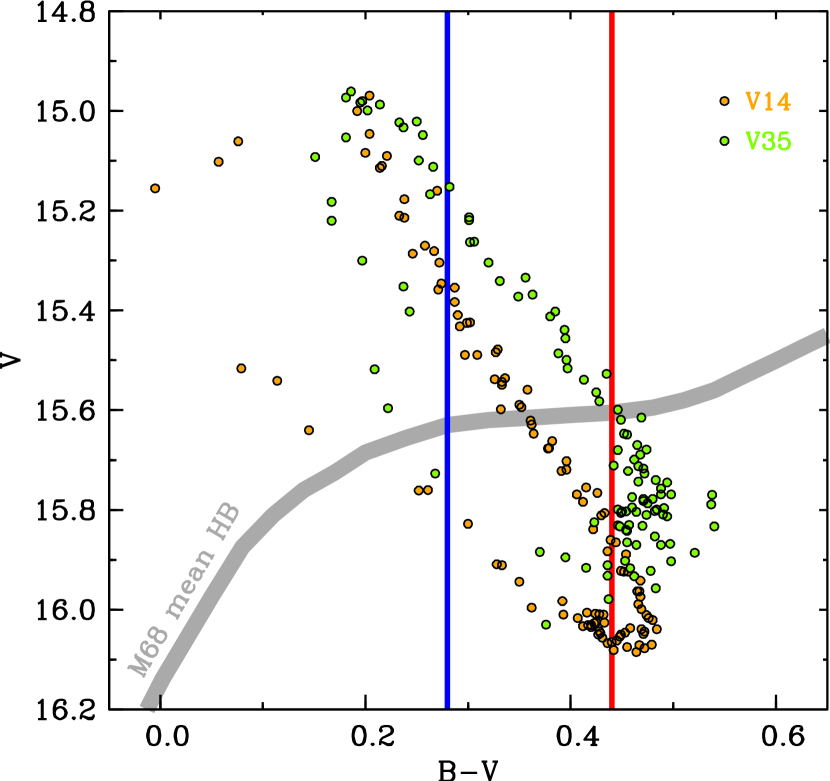
Figure 34: Loops for two RRab stars in the $V$ versus $B-V$ diagram of M68. Orange and green symbols denote data for Walker (1994) variables V14 (P = 0.5568 d) and V35 (P = 0.7025 d), and the grey line is a hand drawn representation of the HB population in M68. Blue and red vertical lines mark the color boundaries of the RR Lyr instability strip estimated from the data points in Walker’s Figure 13.

A recent estimate of the effective temperature at the red edge of the RR Lyrae instability strip, $T_{\rm eff}$(FRE), by Hansen et al. (2011) prompts us to investigate this quantity anew. Hansen et al. adopt $T_{\rm eff}$(FRE) = 5900 K, the effective temperature derived from analysis of spectra of two metal-poor RR Lyr stars observed near minimum light. Their estimate arises from a misunderstanding of the FRE. This is illustrated in Figure 34, where we superpose ($V$, $B-V$) loops for two RRab stars, V14 (P = 0.5568 d) and V35 (P =0.7025 d), on the horizontal branch of the metal-poor ([Fe/H]=-2.2) globular cluster M68. The data are those of Walker (1994). The schematic horizontal branch was hand drawn through the data points in Walker’s Figure 13. Vertical blue and red lines denote boundaries of the instability strip defined approximately by the locations of BHB, RR Lyr, and RHB stars in that Figure. For a considerable portion of the pulsation cycles preceding minimum light, as can be inferred from the densities of data points at faintest apparent magnitudes, the colors of the RR Lyrae stars lie in the RHB domain, well outside of the instability strip. This is a general characteristic of the RRab stars. T(FRE) cannot be derived from observations at these phases alone.

Preston et al. (2006a) obtained their higher value, T(FRE) = 6300 K, by pinching the FRE between the red edge of the color (temperature) distribution of metal-poor RRab stars and the blue edge of the metal-poor RHB distribution at their disposal. For this purpose they used mean colors of RRab stars, employing the formalism of Preston (1961a). This formalism, used to locate RR Lyrae stars in CMDs for many decades, defines the mean color (hence mean $T_{\rm eff}$) of an RR Lyr star as the color of a fictitious static star with the same $T_{\rm eff}$ and absolute luminosity. Variants of the procedure by which this color is calculated are reviewed (with references) by Sandage (2006). The variants produce small differences in the mean colors that are not important for the present discussion.

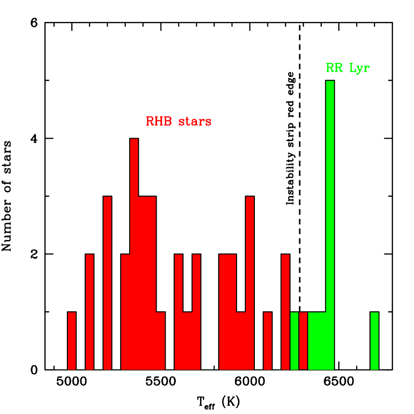
Figure 35: A histogram showing the distribution of $T_{\rm eff}$ values of RHB field stars (red) and mean $T_{\rm eff}$ values for of RR Lyr sample (green). The dashed vertical line represents our best $T_{\rm eff}$ estimate (6280 K) for the FRE.

Here, we follow a procedure similar to that used by Preston et al. (2006a) based on effective temperatures derived from analyses of our RR Lyr spectra. We calculated $T_{\rm eff}$ values at intervals of 0.05 in phase by linear interpolation among the data in Table 5. We used these to calculate the average values of $T_{\rm eff}$ for each star given in Table 13. We omitted TY Gru and V1645 Sgr for which we deemed the data inadequate. We estimated T(FRE) = 6310 K as the average of the two lowest values in Table 13 (for CD Vel and Z Mic). In similar fashion we estimated T(FRE) = 6250 K as the average of the two highest $T_{\rm eff}$ values among the RHB stars of For & Sneden (2010). We adopt $T_{\rm eff}$(FRE) = 6280 $\pm$ 30 K as the average of these two independent estimates. A histogram illustrating the distribution of these RR Lyr and RHB temperatures is presented in Figure 35. Our procedure based on new data is closely equivalent to that of Preston et al., and it produces virtually the same value for $T_{\rm eff}$(FRE), albeit for a sample of somewhat higher mean [Fe/H]. The estimate offered here supersedes the estimate of For & Sneden (2010).

Two puzzles emerge from this discussion: why is there such small dispersion in $<$$T_{\rm eff}$$>$ among the RR Lyr that populate a relatively broad color region of the instability strip, and why do these values crowd the red edge? These are issues for future investigation.

10 EVOLUTIONARY STATES OF THE RR LYR SAMPLE

Horizontal-branch morphology is a complex function of many parameters. The first and most obvious parameter is metallicity, because metal-rich globular clusters have mostly RHB stars while metal-poor globular clusters have mostly BHB and/or EHB stars. The metallicity distributions of the field RHB and BHB samples in For & Sneden (2010) and RRab sample of this study have some differences. More RHB stars agglomerate toward the lower metallicity regime ([Fe/H]$<-2.0$), more BHB stars toward the higher metallicity regime ([Fe/H]$>-1.5$), respectively, and the RRab sample falls in between. These distributions, which confuse arguments about the first parameter of HB morphology, are artificial and arise from observational selection biases. They cannot provide physical interpretation of HB morphology.

In For & Sneden (2010), the majority RHB stars were selected from Preston et al. (2006a), which was a study specifically focused on metal-poor RHB stars. On the other hand, metal-poor BHB stars ([Fe/H]$<-2.0$) were excluded due to the lack of measurable Fe I and Fe II lines for spectroscopic analysis (see comment in Table 2 of For & Sneden, 2010). The RRab stars that were selected for this study partly to better understand the nature of a carbon-rich and $s$-process rich RRab star, TY Gru (Preston et al., 2006b). We refer the reader to the description of selecting RRab stars in this study to FPS11.

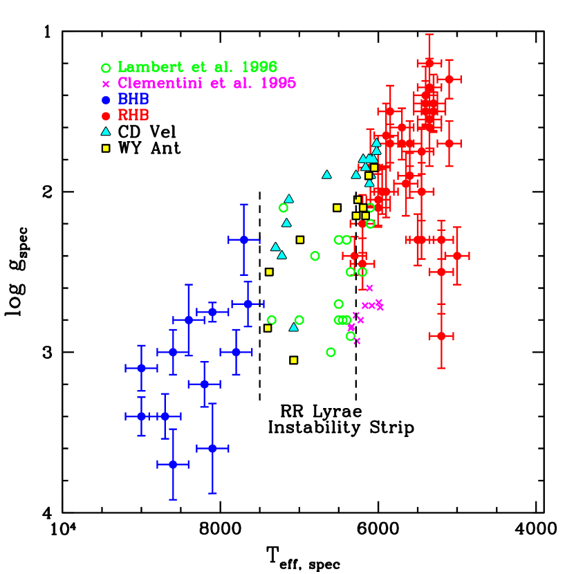
Figure 36: Spectroscopic $T_{\rm eff}$ and log g of CD Vel and WY Ant, with additional data from For & Sneden (2010) (RHB: red dots; BHB: blue dots), Lambert et al. (1996) (green open circles) and Clementini et al. (1995) (magenta crosses) on the $T_{\rm eff}$-log g plane.

With these cautions in mind, we compared the physical properties of our RRab stars with the RR Lyr samples of Lambert et al. (1996) and Clementini et al. (1995). In Figure 36, we extend Figure 19 of For & Sneden (2010) by adding the derived spectroscopic $T_{\rm eff}$ and log g values of two of our RRab stars, CD Vel and WY Ant, on the $T_{\rm eff}$-log g plane. These two stars are selected due to the lower log g of WY Ant throughout the cycle as compared to CD Vel, which provides a small vertical offset for easier visual inspection. The $T_{\rm eff}$ and log g values of field RR Lyr samples are based on the spectroscopic derivations of Lambert et al. (1996), and photometric $T_{\rm eff}$ and Baade-Wesselink log g of Clementini et al. (1995) study. Our log g values derived from spectroscopic ionization balance are generally lower than the Baade-Wesselink method. However, they follow the general physical $T_{\rm eff}$ and log g change with the RHB and BHB population across the $T_{\rm eff}$-log g plane.

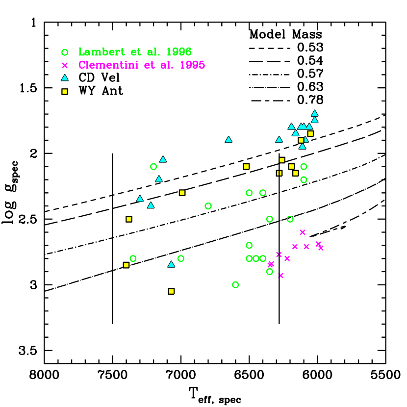
Figure 37: An enlarged version of Figure 36 near the instability strip region with an overlaid of $\alpha$-enhanced HB tracks of [M/H] $=-1.79$, $Z=0.0003$, $Y=0.245$.

In Figure 37, we enlarge Figure 36 near the RR Lyr instability strip region. In this figure we have added $\alpha$-enhanced HB tracks of [M/H]= $-1.79$, $Z=0.0003$ and $Y=0.245$ with different model masses. These HB tracks are adopted from Pietrinferni et al. (2006), which have been implemented with low $T$-opacities of Ferguson et al. (2005) and an $\alpha$-enhanced distribution that represents typical Galactic halo and bulge stars. We employed Eq. 4 to convert the bolometric luminosities in the model to log g values. A large star-to-star scatter for Lambert et al’s data is evident, but our RR Lyrs follow the general trend of a single mass evolutionary track (within log g uncertainties) except near 7000–7500 K region. The scatter in this $T_{\rm eff}$ range is due to the fast moving and complex nature of RR Lyr atmosphere during the rising and descending branch of the cycle. Accepting at face value the large spread in log g implies masses in the entire range from 0.5–0.8 $M_{\odot}$, a conclusion broadly consistent with horizontal branch theory.

11 SUMMARY AND CONCLUSIONS

We present the first detailed chemical abundance study of field horizontal branch RR Lyrae variable stars throughout their pulsational cycles. For this work we gathered some 2300 high resolution spectra of 11 RRab stars with the du Pont 2.5-m telescope at the Las Campanas Observatory. The samples were selected based on the study of Preston (2011). A new, indirect method to estimate initial $T_{\rm eff}$ values for the analysis was developed. These estimated temperatures work reasonably well for both Blazhko and non-Blazhko effect stars.

We derived the model stellar atmospheric parameters, $T_{\rm eff}$, log g, [M/H] and $v_{\rm t}$ for all our program stars throughout the pulsational cycles based on spectroscopic constraints. Variations of microturbulence as a function of $T_{\rm eff}$ and phase were found. We found a variation of $v_{\rm t}$ with $T_{\rm eff}$ along the horizontal branch that goes through a maximum in the RR Lyr instability strip. We also showed for the first time observationally that the variation of $v_{\rm t}$ as a function of phase is similar to the theoretical $v_{\rm t}$ and kinetic energy calculations of Fokin et al. (1999b) and Kolenberg et al. (2010), respectively.

Employing the derived model stellar atmospheric parameters, we obtained abundance ratios, [X/Fe], of the $\alpha$-elements, light odd-$Z$ elements, Fe-peak elements, and $n$-capture elements. The elemental abundance ratios show consistency throughout the pulsational cycles for both Blazhko and non-Blazhko effect stars. The mean abundance ratios vs metallicity of our program stars are also generally in accord with the RHB and BHB stars. We did not obtain satisfactory solution for the known trend of Silicon abundances as a function of $T_{\rm eff}$ with our RR Lyr stars.

Finally, we investigated the physical properties of our RR Lyr stars by comparing them with those presented in Lambert et al. (1996) and Clementini et al. (1995) in the $T_{\rm eff}$-log g plane. A large star-to-star scatter on the $T_{\rm eff}$-log g plane was found for Lambert et al’s samples in contrast to our RR Lyr, which follow the general trend of a single mass evolutionary track. Clementini et al. obtained lower log g values from analysis by the BW method.

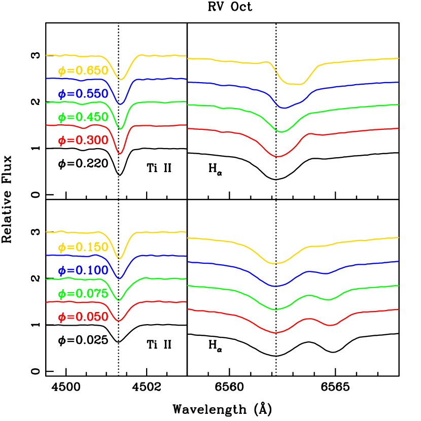
Figure 3: Repeat of Figure 1 for RV Oct, but showing many more combined spectra between $\phi$ = 0.2 and 0.6 where the metal lines remain reasonably sharp with the least asymmetric profile distortion.

Figure 13: Derived stellar parameters ($T_{\rm eff}$, log g, [M/H], and $v_{\rm t}$) for RV Oct based on spectroscopic constraints as a function of phase. The dashed lines in the bottom two panels represent the mean values of [M/H] and $v_{\rm t}$.

Figure 20: Abundance ratios, [X/Fe], of Na I, Mg I, Al I and Si I as a function of phase for the non-Blazhko effect star, RV Oct. The dashed lines represent the mean values. The [X/Fe] values are generally consistent throughout the pulsational cycle. NLTE corrections were applied to Na, Al and Si abundances whenever appropriate. The small trend of [Si I/Fe] between phase 0.8 and 1.0 is discussed in § 8.2.

Figure 21: Same as Figure 20, now for Si II, Ca I, Sc II and Ti I. NLTE corrections applied to Si II abundances whenever appropriate. The trend of [Si II/Fe] is discussed in § 8.2.

Figure 22: Same as Figure 20, now for Ti II, V II, Cr I and Cr II.

Figure 23: Same as Figure 20, now for Co I, Ni I, Y II and Zn I. The large phase-to-phase scatter of [Ni I/Fe] is due to the large uncertainties in the derived values.

Table 1: Basic Information for the Program Stars.

Star	R.A.(J2000)	Decl.(J2000)	Data Used	$T_{0}$	err	Period	err	$N$
	(hr m s)	($\arcdeg$ $\arcmin$ $\arcsec$)	(HJD 2450000+)	(HJD 2450000+)	(HJD 2450000+)	(day)	(day)
CD Vel	09 44 38.24	$-$45 52 37.2	all	3837.632	0.0003	0.573510	0.000003	208
WY Ant	10 16 04.95	$-$29 43 42.4	all	4191.685	0.0097	0.574344	0.000002	136
DT Hya	11 54 00.18	$-$31 15 40.0	all	4583.637	0.0089	0.567978	0.000001	102
AS Vir	12 52 45.86	$-$10 15 36.4	all	4907.709	0.0098	0.553412	0.000002	262
RV Oct	13 46 31.75	$-$84 24 06.4	all	3841.602	0.0016	0.571170	0.000002	222
XZ Aps	14 52 05.43	$-$79 40 46.6	all	3842.735	0.0052	0.587264	0.000002	289
BS Aps	16 20 51.51	$-$71 40 15.8	all	4583.785	0.0045	0.582561	0.000007	252
UV Oct	16 32 25.53	$-$83 54 10.5	3836.84–3842.91, 4306.46–5021.84	3837.875	0.0072	0.542578	0.000003	323
			3931.58–4194.92, 5070.48–5073.59	5070.605	0.0072	$\cdots$	$\cdots$	$\cdots$
V1645 Sgr	20 20 44.47	$-$41 07 05.7	4191.89–4306.90	4306.775	0.0150	0.552948	0.000005	198
			4579.85–4583.91	4579.895	0.0150	$\cdots$	$\cdots$	$\cdots$
			3932.73–3946.75, 4687.66–5074.71	4687.703	0.0170	$\cdots$	$\cdots$	$\cdots$
Z Mic	21 16 22.71	$-$30 17 03.1	all	5075.606	0.0015	0.586926	0.000001	185
TY Gru	22 16 39.42	$-$39 56 18.0	3933.79–3935.65, 5071.50–5073.66	3933.785	0.0120	0.570065	0.000005	114
			3945.63–4306.89	4304.885	0.0120	$\cdots$	$\cdots$	$\cdots$

Table 2: Synthetic Colors for Models with $\log g=2.0$.

	Effective Temperature (K)
Color Indices	5500	5750	6000	6250	6500	6750	7000	7250	7500	7750	8000	8250	8500
[M/H]$=-0.10$ (SW And)
$B-V$	0.755	0.650	0.555	0.470	0.394	0.323	0.249	0.177	0.124	0.081	0.044	0.014	$-$0.007
$V-R_{c}$	0.396	0.352	0.310	0.270	0.230	0.193	0.156	0.120	0.090	0.065	0.044	0.028	0.018
$V-I_{c}$	0.779	0.698	0.620	0.544	0.470	0.397	0.328	0.263	0.206	0.158	0.118	0.087	0.065
[M/H]$=-0.30$ (AR Per)
$B-V$	0.722	0.619	0.528	0.447	0.375	0.307	0.237	0.167	0.115	0.074	0.039	0.011	$-$0.008
$V-R_{c}$	0.390	0.347	0.306	0.266	0.227	0.190	0.153	0.118	0.088	0.064	0.043	0.027	0.017
$V-I_{c}$	0.776	0.697	0.619	0.543	0.470	0.398	0.329	0.264	0.207	0.159	0.119	0.088	0.066
[M/H]$=-1.15$ (RR Leo)
$B-V$	0.612	0.522	0.446	0.380	0.319	0.262	0.204	0.140	0.092	0.056	0.026	0.003	$-$0.011
$V-R_{c}$	0.375	0.334	0.294	0.256	0.218	0.182	0.146	0.112	0.083	0.059	0.040	0.026	0.016
$V-I_{c}$	0.773	0.694	0.618	0.545	0.472	0.401	0.332	0.268	0.210	0.162	0.122	0.092	0.071
[M/H]$=-1.25$ (RR Cet and TU Uma)
$B-V$	0.603	0.515	0.441	0.376	0.316	0.259	0.202	0.138	0.091	0.055	0.026	0.003	$-$0.012
$V-R_{c}$	0.374	0.333	0.294	0.256	0.218	0.182	0.146	0.112	0.083	0.059	0.040	0.026	0.017
$V-I_{c}$	0.773	0.695	0.619	0.545	0.472	0.401	0.332	0.268	0.211	0.162	0.122	0.092	0.072
[M/H]$=-1.35$ (TT Lyn)
$B-V$	0.594	0.508	0.435	0.371	0.312	0.256	0.199	0.136	0.089	0.054	0.025	0.003	$-$0.012
$V-R_{c}$	0.373	0.332	0.293	0.255	0.218	0.181	0.146	0.112	0.082	0.058	0.039	0.026	0.017
$V-I_{c}$	0.773	0.695	0.619	0.545	0.472	0.401	0.332	0.268	0.211	0.162	0.122	0.092	0.072
[M/H]$=-1.40$ (RX Eri)
$B-V$	0.589	0.504	0.432	0.369	0.310	0.255	0.198	0.136	0.088	0.053	0.025	0.002	$-$0.012
$V-R_{c}$	0.367	0.328	0.290	0.252	0.215	0.178	0.143	0.109	0.081	0.057	0.038	0.026	0.018
$V-I_{c}$	0.773	0.695	0.619	0.546	0.473	0.402	0.333	0.269	0.211	0.163	0.123	0.093	0.072
[M/H]$=-1.60$ (SU Dra)
$B-V$	0.574	0.493	0.424	0.362	0.305	0.250	0.195	0.133	0.086	0.051	0.024	0.002	$-$0.012
$V-R_{c}$	0.370	0.330	0.291	0.254	0.217	0.180	0.145	0.111	0.082	0.058	0.039	0.026	0.017
$V-I_{c}$	0.773	0.695	0.619	0.546	0.473	0.402	0.333	0.269	0.211	0.163	0.123	0.094	0.073

Table 3: Basic Data for Deriving the $T_{\rm eff}$–Phase Relations.

Phase	RV$-$RVmin	$B-V$	$c(B-V)$	$T_{\rm eff}$	$V-R_{c}$	$c(V-R_{c})$	$T_{\rm eff}$	$V-I_{c}$	$c(V-I_{c})$	$T_{\rm eff}$
SW And
0.00	0	0.211	0.151	7373	0.131	0.097	7443	0.272	0.198	7544
0.05	2.72	0.237	0.177	7250	0.161	0.127	7203	0.325	0.251	7304
0.10	7.28	0.273	0.213	7125	0.187	0.153	7022	0.377	0.303	7098
0.20	16.83	0.346	0.286	6875	0.226	0.192	6758	0.458	0.384	6799
0.30	26.46	0.453	0.393	6504	0.276	0.242	6426	0.559	0.485	6451
0.40	34.47	0.491	0.431	6378	0.307	0.273	6233	0.614	0.540	6265
0.50	44.89	0.514	0.454	6303	0.318	0.284	6164	0.640	0.566	6179
0.60	48.73	0.526	0.466	6263	0.313	0.279	6195	0.630	0.556	6212
0.75	56.48	0.533	0.473	6241	0.322	0.288	6139	0.643	0.569	6169
0.80	61.36	0.541	0.481	6218	0.319	0.285	6158	0.637	0.563	6189
0.85	62.48	0.495	0.435	6365	0.299	0.265	6283	0.600	0.526	6312
AR Per
0.00	0	0.460	0.140	7380	0.285	0.103	7378	0.597	0.200	7535
0.05	3.56	0.494	0.174	7225	0.311	0.129	7174	0.649	0.252	7301
0.10	7.57	0.528	0.208	7104	0.335	0.153	7003	0.692	0.295	7130
0.20	16.05	0.628	0.308	6746	0.395	0.213	6597	0.820	0.423	6663
0.30	28.04	0.701	0.381	6479	0.431	0.249	6362	0.893	0.496	6410
0.40	35.28	0.743	0.423	6333	0.456	0.274	6203	0.930	0.533	6284
0.50	44.80	0.759	0.439	6278	0.467	0.285	6134	0.956	0.559	6197
0.60	52.40	0.762	0.442	6267	0.469	0.287	6121	0.928	0.531	6290
0.75	58.62	0.762	0.442	6267	0.486	0.304	6015	0.952	0.555	6210
0.80	64.06	0.770	0.450	6241	0.478	0.296	6065	0.936	0.539	6263
0.85	65.73	0.766	0.446	6254	0.467	0.285	6134	0.937	0.540	6260
RR Leo
0.00	0	0.086	0.036	7917	0.057	0.029	8205	0.140	0.078	8417
0.05	5.19	0.097	0.047	7825	0.074	0.046	7927	0.176	0.114	8067
0.10	9.56	0.157	0.107	7421	0.113	0.085	7487	0.241	0.179	7661
0.20	16.79	0.270	0.220	6931	0.197	0.169	6844	0.409	0.347	6946
0.30	29.62	0.341	0.291	6623	0.254	0.226	6451	0.501	0.439	6616
0.40	40.80	0.410	0.360	6332	0.282	0.254	6266	0.587	0.525	6319
0.50	47.49	0.439	0.389	6216	0.298	0.270	6161	0.616	0.554	6219
0.60	54.16	0.435	0.385	6231	0.311	0.283	6076	0.628	0.566	6178
0.70	60.85	0.447	0.397	6186	0.288	0.260	6227	0.603	0.541	6264
0.80	59.28	0.397	0.347	6385	0.285	0.257	6247	0.584	0.522	6329
0.85	59.54	0.424	0.374	6275	0.293	0.265	6194	0.595	0.533	6291
RR Cet
0.00	0	0.171	0.141	7238	0.127	0.110	7268	0.276	0.239	7378
0.05	2.58	0.198	0.168	7133	0.148	0.131	7111	0.322	0.285	7184
0.15	13.17	0.284	0.254	6772	0.206	0.189	6702	0.444	0.407	6730
0.20	17.13	0.320	0.290	6614	0.228	0.211	6549	0.492	0.455	6561
0.30	28.62	0.395	0.365	6296	0.268	0.251	6284	0.559	0.522	6329
0.40	41.56	0.427	0.397	6169	0.282	0.265	6191	0.603	0.566	6180
0.50	45.29	0.447	0.417	6092	0.314	0.297	5981	0.633	0.596	6078
0.60	51.86	0.437	0.407	6131	0.316	0.299	5969	0.625	0.588	6105
0.70	55.11	0.425	0.395	6177	0.302	0.285	6060	0.614	0.577	6143
0.80	57.02	0.440	0.410	6119	0.297	0.280	6093	0.611	0.574	6153
0.85	60.94	0.441	0.411	6115	0.293	0.276	6119	0.602	0.565	6183
TU Uma
0.00	0	0.158	0.138	7250	0.116	0.105	7314	0.265	0.240	7372
0.05	1.07	0.184	0.164	7148	0.142	0.131	7113	0.318	0.293	7152
0.10	1.67	0.237	0.217	6934	0.173	0.162	6892	0.369	0.344	6956
0.20	17.26	0.319	0.299	6575	0.224	0.213	6537	0.476	0.451	6573
0.30	29.74	0.377	0.357	6329	0.276	0.265	6193	0.565	0.540	6266
0.40	37.79	0.418	0.398	6165	0.295	0.284	6068	0.602	0.577	6141
0.50	43.69	0.440	0.420	6081	0.306	0.295	5996	0.618	0.593	6087
0.65	51.18	0.465	0.445	5986	0.288	0.277	6115	0.611	0.586	6111
0.70	52.19	0.446	0.426	6058	0.277	0.266	6187	0.577	0.552	6226
0.80	57.35	0.418	0.398	6165	0.300	0.289	6036	0.605	0.580	6131
0.85	59.37	0.437	0.417	6092	0.284	0.273	6141	0.605	0.580	6131
TT Lyn
0.00	0	0.222	0.212	6943	0.173	0.167	6848	0.368	0.356	6914
0.05	3.11	0.257	0.247	6789	0.190	0.184	6728	0.416	0.404	6741
0.10	6.60	0.285	0.275	6665	0.210	0.204	6593	0.435	0.423	6674
0.20	14.37	0.363	0.353	6326	0.250	0.244	6322	0.517	0.505	6388
0.30	20.75	0.407	0.397	6148	0.270	0.264	6189	0.568	0.556	6214
0.40	33.74	0.426	0.416	6074	0.304	0.298	5966	0.614	0.602	6059
0.50	38.12	0.449	0.439	5986	0.311	0.305	5921	0.625	0.613	6022
0.60	47.08	0.450	0.440	5983	0.308	0.302	5940	0.626	0.614	6018
0.70	47.15	0.430	0.420	6051	0.295	0.289	6024	0.611	0.599	6069
0.80	50.20	0.448	0.438	5990	0.297	0.291	6011	0.619	0.607	6042
0.85	49.79	0.429	0.419	6063	0.304	0.298	5966	0.617	0.605	6049
RX Eri
0.00	0	0.224	0.174	7097	0.158	0.130	7099	0.351	0.289	7172
0.05	3.36	0.250	0.200	6991	0.175	0.147	6975	0.384	0.322	7043
0.10	7.63	0.288	0.238	6825	0.200	0.172	6796	0.438	0.376	6844
0.20	17.49	0.353	0.303	6531	0.271	0.243	6314	0.522	0.460	6546
0.30	27.17	0.445	0.395	6147	0.291	0.263	6181	0.603	0.541	6267
0.40	34.87	0.468	0.418	6056	0.306	0.278	6082	0.650	0.588	6106
0.50	42.02	0.488	0.438	5979	0.323	0.295	5970	0.661	0.599	6069
0.60	47.76	0.501	0.451	5934	0.330	0.302	5924	0.690	0.628	5970
0.70	49.59	0.474	0.424	6032	0.324	0.296	5964	0.665	0.603	6055
0.80	56.47	0.495	0.445	5955	0.331	0.303	5918	0.672	0.610	6031
0.85	58.69	0.473	0.423	6036	0.328	0.300	5938	0.663	0.601	6062
SU Dra
0.00	0	0.143	0.133	7250	0.113	0.107	7282	0.261	0.249	7338
0.05	1.40	0.174	0.164	7125	0.135	0.129	7115	0.306	0.294	7154
0.10	5.49	0.218	0.208	6941	0.174	0.168	6834	0.370	0.358	6911
0.20	16.05	0.287	0.277	6627	0.217	0.211	6539	0.464	0.452	6575
0.30	21.49	0.370	0.360	6259	0.260	0.254	6248	0.550	0.538	6279
0.40	32.49	0.417	0.407	6069	0.287	0.281	6066	0.607	0.595	6084
0.50	40.56	0.430	0.420	6016	0.304	0.298	5953	0.622	0.610	6032
0.60	44.52	0.437	0.427	5989	0.301	0.295	5972	0.622	0.610	6032
0.70	45.85	0.414	0.404	6081	0.291	0.285	6039	0.604	0.592	6094
0.80	53.85	0.411	0.401	6093	0.290	0.284	6045	0.600	0.588	6108
0.85	55.06	0.418	0.408	6065	0.282	0.276	6099	0.597	0.585	6118

Table 4: Coefficients for the Temperature$-$Phase Relationships.

Eq	Star	$a_{4}$	$a_{3}$	$a_{2}$	$a_{1}$	$a_{0}$
1	SW And	$-$1049.6	600.08	4153.8	$-$4808.7	7542.7
2	AR Per	$-$5174.6	4653.8	4167.1	$-$5275.8	7554.7
3	RR Leo	$-$6583.7	5248.0	7718.5	$-$8830.7	8444.6
4	RR Cet	$-$3483.1	2780.7	4418.3	$-$5061.1	7394.3
5	TU Uma	$-$10916	14340	$-$960.06	$-$4324.7	7373.8
6	TT Lyn	$-$7213.9	10633	$-$2121.4	$-$2464.3	6902.5
7	RX Eri	$-$6602.1	9883.2	$-$1303.9	$-$3315.4	7186.2
8	SU Dra	$-$8545.3	12001	$-$860.84	$-$4142.2	7343.4

Table 5: Stellar Atmosphere Parameters and Fe Abundances throughout the Pulsational Cycles.

Mid Phase	$T_{\rm eff}$	err	log g	err	[M/H]	$v_{\rm t}$	err	[Fe I/H]	err	$N$	[Fe II/H]	err	$N$
	(K)		(dex)		(dex)	(km s-1)	(dex)				(dex)
CD Vel
0.015	7130	300	2.05	0.20	$-1.80$	2.85	0.20	$-1.80$	0.09	30	$-1.81$	0.10	25
0.045	7160	300	2.20	0.24	$-1.63$	2.90	0.20	$-1.63$	0.11	26	$-1.62$	0.12	16
0.150	6650	200	1.90	0.16	$-1.74$	2.75	0.30	$-1.74$	0.10	68	$-1.73$	0.08	23
0.300	6280	100	1.90	0.22	$-1.73$	2.50	0.10	$-1.73$	0.11	82	$-1.73$	0.11	29
0.400	6100	100	1.80	0.20	$-1.80$	2.70	0.10	$-1.80$	0.09	80	$-1.80$	0.10	23
0.500	6020	100	1.75	0.20	$-1.83$	2.80	0.10	$-1.83$	0.11	76	$-1.83$	0.10	29
0.570	6020	100	1.70	0.20	$-1.89$	3.20	0.10	$-1.89$	0.09	63	$-1.89$	0.10	20
0.650	6060	100	1.80	0.14	$-1.88$	3.15	0.10	$-1.88$	0.10	55	$-1.89$	0.07	25
0.700	6090	150	1.90	0.24	$-1.86$	3.75	0.20	$-1.86$	0.10	53	$-1.87$	0.12	16
0.750	6110	150	1.95	0.18	$-1.86$	3.80	0.20	$-1.86$	0.09	50	$-1.86$	0.09	19
0.800	6120	150	1.80	0.26	$-1.85$	3.70	0.40	$-1.85$	0.10	49	$-1.86$	0.13	23
0.850	6160	150	1.85	0.24	$-1.90$	3.80	0.40	$-1.90$	0.11	58	$-1.89$	0.12	19
0.900	6190	200	1.80	0.18	$-2.14$	4.00	0.30	$-2.14$	0.11	42	$-2.12$	0.09	15
0.950	7070	300	2.85	0.18	$-1.82$	3.95	0.20	$-1.82$	0.08	35	$-1.82$	0.09	21
0.970	7220	300	2.40	0.18	$-1.85$	3.50	0.20	$-1.85$	0.11	23	$-1.86$	0.09	19
0.990	7300	300	2.35	0.20	$-1.76$	3.30	0.20	$-1.76$	0.11	30	$-1.77$	0.10	18
WY Ant
0.035	7380	300	2.50	0.24	$-1.92$	3.10	0.20	$-1.92$	0.10	29	$-1.92$	0.12	20
0.100	6990	200	2.30	0.20	$-1.88$	3.65	0.40	$-1.89$	0.11	49	$-1.90$	0.10	28
0.230	6520	150	2.10	0.14	$-1.90$	3.35	0.20	$-1.91$	0.09	84	$-1.92$	0.07	33
0.350	6260	100	2.05	0.20	$-1.91$	2.85	0.10	$-1.92$	0.09	101	$-1.93$	0.10	36
0.450	6120	100	1.90	0.24	$-1.95$	2.75	0.10	$-1.95$	0.08	97	$-1.96$	0.12	36
0.550	6160	100	2.15	0.18	$-1.90$	3.00	0.10	$-1.91$	0.10	98	$-1.91$	0.09	33
0.650	6050	100	1.85	0.20	$-2.07$	3.45	0.10	$-2.07$	0.08	78	$-2.06$	0.10	26
0.750	6190	150	2.10	0.14	$-2.02$	3.80	0.20	$-2.02$	0.10	62	$-2.03$	0.07	23
0.850	6280	150	2.15	0.20	$-2.00$	4.00	0.40	$-2.00$	0.09	50	$-2.01$	0.10	26
0.920	7070	200	3.05	0.18	$-1.97$	4.00	0.30	$-1.98$	0.10	32	$-1.99$	0.09	17
0.970	7400	300	2.85	0.26	$-1.87$	3.00	0.20	$-1.87$	0.13	27	$-1.88$	0.13	17
DT Hya
0.023	7160	300	1.95	0.14	$-1.43$	3.45	0.20	$-1.43$	0.11	26	$-1.44$	0.07	18
0.120	6860	200	2.10	0.24	$-1.37$	3.50	0.40	$-1.38$	0.11	50	$-1.39$	0.12	22
0.320	6280	100	2.00	0.28	$-1.37$	2.80	0.10	$-1.38$	0.12	87	$-1.38$	0.14	27
0.500	6100	100	1.80	0.24	$-1.50$	3.00	0.10	$-1.50$	0.10	65	$-1.50$	0.12	25
0.650	6110	100	1.70	0.26	$-1.49$	3.60	0.10	$-1.49$	0.11	44	$-1.50$	0.13	11
0.770	6160	150	2.40	0.06	$-1.25$	3.10	0.20	$-1.25$	0.11	27	$-1.27$	0.03	5
0.860	6180	150	1.90	0.14	$-1.65$	3.80	0.30	$-1.65$	0.13	26	$-1.64$	0.07	8
0.900	6940	200	2.60	0.28	$-1.55$	3.60	0.30	$-1.55$	0.13	37	$-1.55$	0.14	13
0.960	7200	300	2.05	0.22	$-1.58$	3.50	0.20	$-1.58$	0.10	41	$-1.59$	0.11	23
AS Vir 1
0.050	6780	300	1.65	0.18	$-1.85$	3.10	0.20	$-1.84$	0.08	25	$-1.84$	0.09	14
0.180	6450	200	1.70	0.22	$-1.67$	3.00	0.30	$-1.67$	0.08	46	$-1.67$	0.11	20
0.320	6170	100	1.85	0.22	$-1.65$	2.90	0.10	$-1.65$	0.10	78	$-1.65$	0.11	30
0.450	6040	100	1.65	0.20	$-1.67$	2.70	0.10	$-1.66$	0.09	64	$-1.67$	0.10	23
0.550	6010	100	1.85	0.22	$-1.73$	2.90	0.10	$-1.73$	0.09	55	$-1.72$	0.11	17
0.650	6040	100	1.80	0.20	$-1.74$	3.50	0.10	$-1.74$	0.09	44	$-1.74$	0.10	11
0.800	6040	150	1.55	0.20	$-1.78$	3.80	0.20	$-1.78$	0.11	38	$-1.79$	0.10	8
0.830	6050	150	1.80	0.18	$-1.86$	3.90	0.40	$-1.86$	0.07	30	$-1.86$	0.09	5
0.880	6490	200	2.50	0.22	$-1.86$	4.45	0.30	$-1.86$	0.11	16	$-1.87$	0.11	2
0.910	6670	200	2.20	0.22	$-1.91$	3.10	0.30	$-1.91$	0.11	17	$-1.92$	0.11	6
0.960	6960	300	2.10	0.22	$-1.81$	2.75	0.20	$-1.82$	0.11	16	$-1.81$	0.11	11
0.980	6850	300	1.75	0.22	$-1.90$	2.60	0.20	$-1.90$	0.13	25	$-1.89$	0.11	12
AS Vir 2
0.030	7090	300	1.40	0.20	$-1.85$	3.40	0.20	$-1.85$	0.10	11	$-1.86$	0.10	15
0.140	6720	200	1.60	0.22	$-1.64$	3.20	0.30	$-1.65$	0.06	31	$-1.65$	0.11	11
0.250	6290	100	1.85	0.20	$-1.68$	2.75	0.20	$-1.68$	0.11	38	$-1.68$	0.10	13
0.350	6030	100	1.55	0.20	$-1.78$	3.00	0.10	$-1.78$	0.09	70	$-1.78$	0.10	21
0.490	6030	100	1.75	0.18	$-1.70$	3.00	0.10	$-1.70$	0.08	65	$-1.70$	0.09	20
0.700	6030	150	1.75	0.12	$-1.82$	4.00	0.20	$-1.82$	0.09	50	$-1.82$	0.06	16
0.850	6050	150	1.75	0.16	$-1.86$	3.90	0.40	$-1.86$	0.10	40	$-1.87$	0.08	16
RV Oct
0.025	7440	300	2.00	0.18	$-1.50$	3.05	0.20	$-1.50$	0.10	44	$-1.51$	0.09	30
0.050	7150	300	1.45	0.26	$-1.57$	3.00	0.20	$-1.57$	0.10	46	$-1.58$	0.13	25
0.075	7040	200	1.60	0.22	$-1.58$	3.50	0.40	$-1.58$	0.09	33	$-1.59$	0.11	23
0.100	6990	200	1.70	0.16	$-1.51$	3.60	0.40	$-1.50$	0.10	43	$-1.50$	0.08	25
0.150	6740	200	1.80	0.26	$-1.45$	3.50	0.30	$-1.46$	0.10	48	$-1.47$	0.13	20
0.220	6520	150	2.00	0.18	$-1.46$	3.00	0.20	$-1.46$	0.11	91	$-1.45$	0.09	33
0.300	6320	100	2.00	0.22	$-1.44$	3.00	0.10	$-1.44$	0.10	99	$-1.44$	0.11	37
0.450	6070	100	1.85	0.28	$-1.48$	2.50	0.10	$-1.50$	0.11	92	$-1.51$	0.14	25
0.550	6090	100	1.95	0.22	$-1.53$	3.00	0.10	$-1.53$	0.13	63	$-1.52$	0.11	21
0.650	6110	100	2.00	0.18	$-1.57$	3.50	0.10	$-1.57$	0.09	67	$-1.57$	0.09	19
0.700	6130	150	2.00	0.24	$-1.50$	3.50	0.20	$-1.50$	0.11	70	$-1.49$	0.12	19
0.750	6160	150	1.90	0.24	$-1.42$	3.50	0.20	$-1.42$	0.10	54	$-1.41$	0.12	19
0.830	6180	150	2.05	0.22	$-1.45$	3.60	0.40	$-1.46$	0.10	75	$-1.45$	0.11	20
0.900	6160	200	1.70	0.22	$-1.69$	3.40	0.30	$-1.69$	0.10	50	$-1.69$	0.11	21
0.930	7060	200	2.70	0.18	$-1.64$	3.50	0.40	$-1.64$	0.11	38	$-1.63$	0.09	14
0.950	7390	300	2.45	0.20	$-1.66$	3.10	0.20	$-1.66$	0.07	29	$-1.67$	0.10	18
0.980	7550	300	1.90	0.20	$-1.62$	3.50	0.20	$-1.62$	0.10	19	$-1.63$	0.10	19
XZ Aps
0.017	7310	300	1.45	0.20	$-2.00$	3.50	0.20	$-2.00$	0.09	6	$-2.02$	0.10	15
0.045	7280	300	1.60	0.28	$-1.89$	3.70	0.20	$-1.86$	0.12	15	$-1.88$	0.14	17
0.075	7040	200	1.60	0.22	$-1.90$	3.70	0.40	$-1.88$	0.13	27	$-1.91$	0.11	25
0.120	6860	200	1.60	0.20	$-1.89$	3.70	0.40	$-1.87$	0.10	42	$-1.88$	0.10	35
0.200	6580	150	1.85	0.20	$-1.76$	3.00	0.20	$-1.76$	0.10	60	$-1.75$	0.10	23
0.320	6280	100	1.85	0.22	$-1.80$	3.00	0.10	$-1.80$	0.10	78	$-1.80$	0.11	25
0.480	6100	100	1.80	0.16	$-1.90$	3.00	0.10	$-1.87$	0.09	65	$-1.89$	0.08	27
0.600	6100	100	1.80	0.22	$-1.90$	3.40	0.10	$-1.92$	0.10	62	$-1.92$	0.11	17
0.680	6130	100	2.00	0.16	$-1.97$	3.90	0.20	$-1.97$	0.09	46	$-1.99$	0.08	12
0.740	6060	150	1.85	0.20	$-1.93$	3.95	0.20	$-1.93$	0.10	44	$-1.93$	0.10	16
0.780	6090	150	1.95	0.24	$-1.82$	3.85	0.20	$-1.87$	0.09	43	$-1.84$	0.12	17
0.810	5970	150	1.70	0.16	$-1.99$	4.45	0.40	$-1.99$	0.10	38	$-2.01$	0.08	13
0.820	6170	150	2.05	0.24	$-1.84$	3.90	0.40	$-1.84$	0.09	39	$-1.86$	0.12	21
0.860	6170	150	1.90	0.24	$-1.89$	3.90	0.30	$-1.89$	0.09	42	$-1.92$	0.12	21
0.890	6200	200	2.00	0.14	$-2.01$	4.35	0.30	$-2.00$	0.10	41	$-2.00$	0.07	13
0.910	6700	200	2.75	0.28	$-1.78$	3.60	0.30	$-1.78$	0.09	25	$-1.80$	0.14	6
0.920	7020	200	2.40	0.22	$-1.83$	3.70	0.40	$-1.83$	0.12	16	$-1.84$	0.11	5
0.950	7340	300	2.30	0.26	$-1.91$	3.85	0.20	$-1.92$	0.13	13	$-1.92$	0.13	14
0.970	7540	300	2.35	0.18	$-1.97$	4.00	0.20	$-1.97$	0.11	13	$-1.98$	0.09	14
0.980	7560	300	2.15	0.22	$-2.00$	3.60	0.20	$-2.00$	0.09	13	$-1.99$	0.11	11
BS Aps 1
0.030	7120	300	2.00	0.26	$-1.35$	3.05	0.20	$-1.35$	0.09	34	$-1.36$	0.13	16
0.130	6700	200	2.15	0.22	$-1.37$	3.15	0.30	$-1.37$	0.10	52	$-1.38$	0.11	25
0.300	6230	100	1.90	0.26	$-1.40$	3.05	0.10	$-1.40$	0.12	74	$-1.40$	0.13	28
0.520	6090	100	1.85	0.26	$-1.47$	3.10	0.10	$-1.47$	0.11	75	$-1.47$	0.13	20
0.730	6140	150	2.15	0.14	$-1.44$	3.90	0.20	$-1.44$	0.09	43	$-1.45$	0.07	11
0.850	6170	150	1.90	0.24	$-1.54$	3.70	0.30	$-1.54$	0.10	42	$-1.54$	0.12	13
0.900	6830	200	2.80	0.26	$-1.47$	3.55	0.30	$-1.47$	0.12	34	$-1.47$	0.13	11
0.950	7010	300	2.60	0.22	$-1.45$	3.15	0.20	$-1.45$	0.11	40	$-1.46$	0.11	19
0.980	7190	300	2.25	0.24	$-1.41$	3.45	0.20	$-1.41$	0.10	34	$-1.42$	0.12	20
BS Aps 2
0.020	7000	300	2.25	0.18	$-1.45$	3.15	0.20	$-1.45$	0.10	33	$-1.46$	0.09	21
0.250	6290	100	1.90	0.24	$-1.49$	2.90	0.20	$-1.49$	0.11	70	$-1.49$	0.12	27
0.650	6040	100	1.80	0.22	$-1.55$	3.40	0.10	$-1.55$	0.10	52	$-1.54$	0.11	21
0.820	6060	150	1.85	0.20	$-1.60$	3.70	0.40	$-1.60$	0.10	60	$-1.59$	0.10	14
0.880	6160	200	1.75	0.20	$-1.80$	4.25	0.30	$-1.80$	0.11	43	$-1.80$	0.10	19
0.930	6700	200	2.35	0.22	$-1.60$	3.50	0.40	$-1.60$	0.10	48	$-1.59$	0.11	23
0.980	6850	300	2.40	0.20	$-1.49$	3.00	0.20	$-1.49$	0.11	46	$-1.48$	0.10	24
BS Aps 3
0.100	6550	200	2.10	0.22	$-1.54$	3.65	0.40	$-1.54$	0.11	30	$-1.54$	0.11	24
0.920	6590	200	2.35	0.20	$-1.52$	3.45	0.30	$-1.52$	0.09	46	$-1.53$	0.10	17
UV Oct 1
0.025	7430	300	2.05	0.20	$-1.66$	3.80	0.20	$-1.66$	0.08	21	$-1.66$	0.10	22
0.077	7080	200	2.00	0.18	$-1.63$	3.75	0.40	$-1.64$	0.08	33	$-1.64$	0.09	21
0.190	6240	150	1.75	0.20	$-1.76$	2.80	0.30	$-1.76$	0.09	87	$-1.77$	0.10	28
0.560	6000	100	1.80	0.20	$-1.82$	3.40	0.10	$-1.82$	0.08	71	$-1.81$	0.10	21
0.740	6220	150	2.00	0.24	$-1.71$	3.85	0.20	$-1.70$	0.10	69	$-1.71$	0.12	21
0.820	6250	150	2.10	0.18	$-1.71$	4.00	0.30	$-1.72$	0.07	57	$-1.73$	0.09	20
0.870	6220	200	2.00	0.22	$-1.94$	3.10	0.30	$-1.95$	0.07	41	$-1.94$	0.11	15
0.920	7160	200	2.60	0.22	$-1.93$	2.80	0.30	$-1.93$	0.08	32	$-1.94$	0.11	19
0.950	7550	300	1.75	0.22	$-1.95$	3.10	0.20	$-1.95$	0.10	16	$-1.96$	0.11	16
0.980	7630	300	2.00	0.18	$-1.74$	3.55	0.20	$-1.75$	0.10	13	$-1.75$	0.09	16
UV Oct 2
0.023	6850	300	1.90	0.22	$-1.81$	2.50	0.20	$-1.81$	0.07	45	$-1.80$	0.11	29
0.070	6720	200	1.85	0.20	$-1.77$	2.50	0.40	$-1.77$	0.09	58	$-1.76$	0.10	29
0.250	6290	150	1.90	0.22	$-1.73$	2.50	0.20	$-1.73$	0.09	75	$-1.73$	0.11	30
0.600	6020	100	1.80	0.20	$-1.86$	3.00	0.10	$-1.86$	0.09	65	$-1.85$	0.10	27
0.780	6070	150	1.80	0.16	$-1.83$	3.50	0.20	$-1.83$	0.09	66	$-1.84$	0.08	28
0.830	6170	150	1.85	0.22	$-1.89$	3.25	0.40	$-1.89$	0.08	53	$-1.88$	0.11	21
0.870	6800	150	2.65	0.22	$-1.80$	3.50	0.30	$-1.80$	0.08	40	$-1.80$	0.11	19
0.910	6850	200	2.45	0.16	$-1.80$	3.05	0.30	$-1.80$	0.09	36	$-1.81$	0.08	18
0.930	6880	200	2.15	0.24	$-1.87$	3.05	0.40	$-1.88$	0.08	44	$-1.87$	0.12	21
0.970	6960	300	1.90	0.20	$-1.89$	3.00	0.20	$-1.89$	0.08	40	$-1.90$	0.10	25
V1645 Sgr 1
0.170	6470	200	1.80	0.16	$-1.99$	2.80	0.30	$-1.99$	0.10	49	$-1.98$	0.08	14
0.500	6020	100	1.50	0.24	$-2.10$	2.90	0.10	$-2.10$	0.11	27	$-2.10$	0.12	12
0.720	6060	150	1.60	0.20	$-2.21$	3.80	0.20	$-2.21$	0.10	30	$-2.21$	0.10	11
0.820	6060	150	1.65	0.18	$-2.19$	3.40	0.40	$-2.19$	0.09	28	$-2.20$	0.09	15
0.880	6750	200	2.35	0.20	$-1.83$	3.45	0.30	$-1.83$	0.10	20	$-1.83$	0.10	9
0.960	6800	300	1.85	0.24	$-2.12$	3.00	0.20	$-2.12$	0.10	24	$-2.12$	0.12	17
V1645 Sgr 2
0.020	6850	300	1.70	0.20	$-2.06$	3.00	0.20	$-2.06$	0.08	33	$-2.06$	0.10	18
0.700	6050	150	1.70	0.18	$-2.15$	3.50	0.20	$-2.15$	0.07	37	$-2.15$	0.09	14
0.850	6240	200	1.65	0.22	$-2.24$	3.25	0.40	$-2.24$	0.06	23	$-2.24$	0.11	10
0.950	6980	300	1.85	0.20	$-2.09$	2.55	0.20	$-2.09$	0.08	25	$-2.09$	0.10	14
V1645 Sgr 3
0.050	7780	300	2.20	0.24	$-1.71$	2.70	0.20	$-1.71$	0.10	7	$-1.71$	0.12	11
0.140	6250	200	1.15	0.20	$-2.33$	3.80	0.30	$-2.33$	0.09	15	$-2.32$	0.10	15
0.250	6480	100	1.85	0.16	$-1.92$	2.95	0.10	$-1.92$	0.08	53	$-1.92$	0.08	15
0.400	6290	100	2.10	0.20	$-1.81$	3.00	0.10	$-1.81$	0.12	50	$-1.80$	0.10	18
0.750	6100	150	1.75	0.28	$-1.98$	3.25	0.20	$-1.98$	0.09	17	$-1.98$	0.14	2
0.860	6170	150	1.90	0.18	$-2.00$	3.75	0.40	$-2.00$	0.09	29	$-2.00$	0.09	7
Z Mic
0.030	6830	300	2.00	0.22	$-1.53$	3.20	0.20	$-1.53$	0.07	60	$-1.54$	0.11	27
0.140	6310	200	1.55	0.24	$-1.62$	2.90	0.30	$-1.62$	0.09	63	$-1.63$	0.12	26
0.250	6190	100	1.80	0.22	$-1.50$	2.65	0.20	$-1.50$	0.09	72	$-1.51$	0.11	22
0.420	6060	100	1.80	0.24	$-1.46$	2.90	0.10	$-1.46$	0.11	81	$-1.47$	0.12	24
0.530	6010	100	1.75	0.20	$-1.53$	3.20	0.10	$-1.54$	0.10	52	$-1.53$	0.10	18
0.650	6040	100	1.90	0.18	$-1.56$	3.60	0.10	$-1.56$	0.09	65	$-1.57$	0.09	22
0.750	6060	150	1.90	0.16	$-1.54$	3.90	0.20	$-1.54$	0.10	66	$-1.54$	0.08	21
0.830	6050	150	2.05	0.18	$-1.56$	3.60	0.40	$-1.56$	0.11	63	$-1.57$	0.09	17
0.870	6150	150	1.90	0.20	$-1.70$	3.85	0.30	$-1.70$	0.08	47	$-1.70$	0.10	23
0.900	6530	200	2.50	0.20	$-1.64$	3.75	0.30	$-1.64$	0.09	51	$-1.64$	0.10	13
0.920	6700	200	2.55	0.24	$-1.55$	3.00	0.30	$-1.55$	0.10	57	$-1.55$	0.12	21
0.950	6780	300	2.40	0.22	$-1.55$	3.40	0.20	$-1.55$	0.11	53	$-1.55$	0.11	25
0.970	6830	300	2.30	0.20	$-1.54$	3.20	0.20	$-1.54$	0.08	43	$-1.54$	0.10	23
0.990	6880	300	2.00	0.24	$-1.50$	2.70	0.20	$-1.50$	0.08	43	$-1.50$	0.12	18
TY Gru
0.014	7320	300	2.35	0.22	$-1.91$	3.00	0.20	$-1.90$	0.10	3	$-1.91$	0.11	5
0.460	6120	100	2.05	0.24	$-1.96$	3.30	0.10	$-1.95$	0.13	45	$-1.96$	0.12	14
0.800	6360	150	2.05	0.30	$-1.95$	4.15	0.40	$-1.95$	0.12	26	$-1.95$	0.15	10
0.920	6740	200	2.30	0.28	$-1.99$	4.35	0.40	$-1.99$	0.11	17	$-1.99$	0.14	8
0.980	7560	300	2.15	0.36	$-2.16$	4.50	0.20	$-2.16$	0.14	7	$-2.16$	0.18	6

Table 6: HD 140283 $T_{\rm eff}$ and log g Values from Various Studies.

Reference	Method	$T_{\rm eff}$	log g	[Fe/H]
		(K)	(dex)	(dex)
Aoki et al. (2002)	Spectroscopic (Ti $\&$ Fe)	5750	3.3	$-2.58$
Hosford et al. (2009)	Spectroscopic (Fe)	5573$\pm$75	3.1$\pm$0.15	$-2.54$
Asplund et al. (2006)	Balmer line wing fitting	5753$\pm$30	3.7$\pm$0.04	$-2.40$
Ryan et al. (1996)	Photometry	5750	3.4	$-2.54$
Alonso et al. (1996)	Infrared flux	5691$\pm$69	4.0$\pm$0.50	$\cdots$
This study	Spectroscopic (Fe)	5400$\pm$150	2.6$\pm$0.16	$-2.80$
This study	Spectroscopic (Fe)	5400$\pm$150	2.6$\pm$0.16	$-2.80$
This study	Trigonometric	5400	3.7	$-2.94$

Table 7: Abundance ratios of Na, Mg, Al, Si and Ca throughout the Pulsational Cycles.

Phase	[Na I/Fe]	$\sigma$	$N$	[Mg I/Fe]	$\sigma$	$N$	[Al I/Fe]	$\sigma$	$N$	[Si I/Fe]	$\sigma$	$N$	[Si II/Fe]	$\sigma$	$N$	[Ca I/Fe]	$\sigma$	$N$
CD Vel
0.015	$-$0.37	0.03	2	0.40	0.02	3	0.03	$\cdots$	1	$\cdots$	$\cdots$	$\cdots$	0.58	$\cdots$	1	0.19	0.09	8
0.045	$-$0.23	0.07	2	0.31	0.04	2	0.26	$\cdots$	1	$\cdots$	$\cdots$	$\cdots$	0.31	$\cdots$	1	0.22	0.10	7
0.150	$\cdots$	$\cdots$	$\cdots$	0.44	0.03	2	0.18	0.08	2	$\cdots$	$\cdots$	$\cdots$	0.47	$\cdots$	1	0.26	0.06	11
0.300	$\cdots$	$\cdots$	$\cdots$	0.41	0.06	2	0.48	0.22	2	0.66	$\cdots$	1	$\cdots$	$\cdots$	$\cdots$	0.33	0.10	13
.	.	.	.	.	.	.	.	.	.	.	.	.	.	.	.	.	.	.
.	.	.	.	.	.	.	.	.	.	.	.	.	.	.	.	.	.	.
.	.	.	.	.	.	.	.	.	.	.	.	.	.	.	.	.	.	.

Note. — Table 7 is published in its entirety in the electronic edition of the Astrophysical Journal Supplement Series. A portion is shown here for guidance regarding its form and content.

Table 8: Abundance Ratios of Sc, Ti, V and Cr throughout the Pulsational Cycles.

Phase	[Sc II/Fe]	$\sigma$	$N$	[Ti I/Fe]	$\sigma$	$N$	[Ti II/Fe]	$\sigma$	$N$	[V II/Fe]	$\sigma$	$N$	[Cr I/Fe]	$\sigma$	$N$	[Cr II/Fe]	$\sigma$	$N$
CD Vel
0.015	0.24	0.10	3	$\cdots$	$\cdots$	$\cdots$	0.41	0.11	10	$\cdots$	$\cdots$	$\cdots$	$-$0.09	0.12	3	0.21	0.11	3
0.045	0.15	0.01	2	$\cdots$	$\cdots$	$\cdots$	0.31	0.12	13	$\cdots$	$\cdots$	$\cdots$	$-$0.12	0.13	4	0.16	0.13	6
0.150	0.06	0.05	3	0.30	0.05	3	0.27	0.14	17	0.08	$\cdots$	1	$-$0.03	0.11	3	0.05	0.15	7
0.300	0.07	0.04	3	0.29	0.13	4	0.35	0.18	17	0.18	$\cdots$	1	0.07	0.14	5	0.03	0.13	7
.	.	.	.	.	.	.	.	.	.	.	.	.	.	.	.	.	.	.
.	.	.	.	.	.	.	.	.	.	.	.	.	.	.	.	.	.	.
.	.	.	.	.	.	.	.	.	.	.	.	.	.	.	.	.	.	.

Note. — Table 7 is published in its entirety in the electronic edition of the Astrophysical Journal Supplement Series. A portion is shown here for guidance regarding its form and content.

Table 9: Abundance ratios of Co, Ni, Zn and Y throughout the Pulsational Cycles.

Phase	[Co I/Fe]	$\sigma$	$N$	[Ni I/Fe]	$\sigma$	$N$	[Zn I/Fe]	$\sigma$	$N$	[Y II/Fe]	$\sigma$	$N$
CD Vel
0.015	$\cdots$	$\cdots$	$\cdots$	$\cdots$	$\cdots$	$\cdots$	$\cdots$	$\cdots$	$\cdots$	$\cdots$	$\cdots$	$\cdots$
0.045	$\cdots$	$\cdots$	$\cdots$	$\cdots$	$\cdots$	$\cdots$	$\cdots$	$\cdots$	$\cdots$	$-$0.06	$\cdots$	1
0.150	0.05	$\cdots$	1	$\cdots$	$\cdots$	$\cdots$	$\cdots$	$\cdots$	$\cdots$	0.11	0.14	2
0.300	$-$0.01	$\cdots$	1	0.70	$\cdots$	1	0.10	0.01	2	$-$0.18	0.15	2
.	.	.	.	.	.	.	.	.	.	.	.	.
.	.	.	.	.	.	.	.	.	.	.	.	.
.	.	.	.	.	.	.	.	.	.	.	.	.

Note. — Table 7 is published in its entirety in the electronic edition of the Astrophysical Journal Supplement Series. A portion is shown here for guidance regarding its form and content.

Table 10: Abundance Ratios of Mn, Sr, Zr, Ba, La and Eu Derived from Synthetic Spectra.

Star	Phase	[Mn I/Fe]	$\sigma$	$N$	[Sr II/Fe]	$\sigma$	$N$	[Zr II/Fe]	$\sigma$	$N$	[Ba II/Fe]	$\sigma$	$N$	[La II/Fe]	$\sigma$	$N$	[Eu II/Fe]	$\sigma$	$N$
CD Vel	0.30	$-$0.48	0.15	3	0.57	0.21	2	0.36	0.14	2	0.06	0.17	3	$\cdots$	$\cdots$	$\cdots$	0.25	$\cdots$	2
WY Ant	0.35	$-$0.59	$\cdots$	2	0.54	0.07	2	0.48	0.14	2	0.14	0.24	3	0.26	0.14	2	0.62	$\cdots$	2
DT Hya	0.32	$-$0.57	0.14	2	0.72	0.14	2	0.48	$\cdots$	1	0.36	0.13	4	0.04	0.13	2	0.27	$\cdots$	1
AS Vir	0.32,0.35	$-$0.48	0.23	6	0.33	0.33	4	0.31	0.22	5	0.04	0.12	8	0.16	0.20	4	0.51	0.16	3
RV Oct	0.30	$-$0.34	0.15	4	0.57	0.21	2	0.61	0.12	3	0.06	0.15	4	$-$0.06	$\cdots$	1	0.18	$\cdots$	1
XZ Aps	0.32	$-$0.58	0.15	3	0.20	$\cdots$	2	0.72	$\cdots$	1	0.17	0.15	3	$\cdots$	$\cdots$	$\cdots$	$-$0.10	$\cdots$	1
BS Aps	0.30	$-$0.04	0.15	4	0.52	0.21	2	0.57	0.21	2	0.24	0.21	2	$-$0.13	$\cdots$	1	0.17	0.07	2
UV Oct	0.25	$-$0.53	0.14	2	0.20	$\cdots$	2	0.28	0.14	2	0.11	0.21	2	0.05	$\cdots$	2	0.35	$\cdots$	2
V1645 Sgr	0.25	$-$0.52	0.07	2	$-$0.05	$\cdots$	2	0.22	0.15	3	0.02	0.10	3	0.44	0.14	2	0.51	$\cdots$	1
Z Mic	0.25	$-$0.56	0.25	3	0.43	0.07	2	0.20	0.21	2	0.26	0.21	2	0.12	0.07	2	0.37	$\cdots$	1
TY Gru	0.46	$-$0.64	$\cdots$	1	0.04	0.07	2	0.32	$\cdots$	1	1.05	0.17	3	0.85	0.21	2	$\cdots$	$\cdots$	$\cdots$

Table 11: Mean Abundance Ratios for Each Star.

	CD Vel	WY Ant	DT Hya	AS Vir	RV Oct	XZ Aps	BS Aps	UV Oct	V1645 Sgr	Z Mic	TY Gru
Na I	$-$0.37	$-$0.39	$\cdots$	$\cdots$	$-$0.12	$-$0.18	0.08	$-$0.38	$\cdots$	0.12	$\cdots$
$N$	3	3	$\cdots$	$\cdots$	9	8	2	9	$\cdots$	2	$\cdots$
Mg I	0.41	0.39	0.52	0.48	0.59	0.54	0.49	0.44	0.44	0.59	0.38
$N$	16	11	9	19	17	20	18	20	16	14	4
Al I	0.20	0.30	0.41	0.35	0.26	0.42	0.59	0.27	0.25	0.59	0.42
$N$	10	9	2	3	2	4	3	12	6	3	1
Si I	0.61	0.26	0.52	0.63	0.41	0.53	0.59	0.19	$\cdots$	0.59	$\cdots$
$N$	3	6	2	2	14	2	6	10	$\cdots$	8	$\cdots$
Si II	0.41	0.33	0.57	0.47	0.62	0.59	0.49	0.54	0.49	0.58	0.67
$N$	11	11	6	14	17	14	17	19	11	13	2
Ca I	0.34	0.34	0.32	0.39	0.37	0.41	0.3	0.33	0.37	0.32	0.37
$N$	16	11	9	18	17	19	18	20	14	14	3
Ti I	0.35	0.42	0.42	0.35	0.35	0.39	0.39	0.34	0.41	0.45	0.66
$N$	11	7	6	12	14	11	12	10	8	14	2
Ti II	0.29	0.31	0.29	0.22	0.26	0.33	0.28	0.24	0.23	0.3	0.19
$N$	16	11	8	19	17	20	18	20	16	14	5
Sc II	0.13	0.21	0.10	0.06	0.08	0.14	0.11	0.07	0.07	0.09	0.02
$N$	16	11	9	17	17	17	18	20	13	14	5
Cr I	$-$0.04	$-$0.04	$-$0.09	$-$0.08	$-$0.13	$-$0.03	$-$0.11	$-$0.10	$-$0.11	$-$0.11	$-$0.25
$N$	16	11	9	18	17	19	18	20	15	14	4
Cr II	0.11	0.13	0.07	0.12	0.05	0.17	$-$0.02	0.13	0.15	$-$0.07	0.2
$N$	16	11	9	18	17	18	18	20	15	13	5
V II	0.15	0.11	0.39	0.18	0.26	0.35	$\cdots$	$\cdots$	$\cdots$	0.06	$\cdots$
$N$	3	4	1	1	2	1	$\cdots$	$\cdots$	$\cdots$	5	$\cdots$
Mn I	$-$0.48	$-$0.59	$-$0.57	$-$0.48	$-$0.34	$-$0.58	$-$0.04	$-$0.53	$-$0.52	$-$0.56	$-$0.64
$N$	3	2	2	6	4	3	4	2	2	3	1
Co I	0.04	0.14	0.19	0.05	0.09	0.19	0.1	$-$0.01	0.04	$-$0.03	0.16
$N$	6	4	1	4	4	3	9	3	3	2	1
Ni I	0.67	0.34	0.50	0.38	0.24	0.46	0.55	0.59	0.48	0.49	$\cdots$
$N$	3	6	4	9	9	4	4	6	2	10	$\cdots$
Zn I	0.10	0.12	0.09	0.15	0.20	0.14	0.19	0.10	0.17	0.22	0.24
$N$	4	6	3	6	10	4	9	6	1	12	1
Sr II	0.57	0.54	0.72	0.33	0.57	0.20	0.52	0.20	$-$0.05	0.43	0.04
$N$	2	2	2	4	2	2	2	2	2	2	2
Y II	$-$0.05	0.02	0.06	$-$0.02	0.07	0.15	0.03	$-$0.16	$-$0.15	0.08	0.43
$N$	12	8	8	13	15	13	15	11	3	12	2
Zr II	0.36	0.48	0.48	0.31	0.61	0.72	0.57	0.28	0.22	0.20	0.32
$N$	2	2	1	5	3	1	2	2	3	2	1
Ba II	0.06	0.14	0.36	0.04	0.06	0.17	0.24	0.11	0.02	0.26	1.05
$N$	3	3	4	8	4	3	2	2	3	2	3
La II	$\cdots$	0.26	0.04	0.16	$-$0.06	$\cdots$	$-$0.13	0.05	0.44	0.12	0.85
$N$	$\cdots$	2	2	4	1	$\cdots$	1	2	2	2	2
Eu II	0.25	0.62	0.27	0.51	0.18	$-$0.10	0.17	0.35	0.51	0.37	$\cdots$
$N$	2	2	1	3	1	1	2	2	1	1	$\cdots$
$[$Fe I/H$]$	$-$1.83	$-$1.95	$-$1.47	$-$1.78	$-$1.54	$-$1.90	$-$1.50	$-$1.81	$-$2.06	$-$1.56	$-$1.99
$N$	16	11	9	19	17	20	15	20	16	14	5
$[$Fe II/H$]$	$-$1.83	$-$1.96	$-$1.47	$-$1.78	$-$1.54	$-$1.91	$-$1.50	$-$1.81	$-$2.06	$-$1.56	$-$1.99
$N$	16	11	9	19	17	20	15	20	16	14	5

Table 12: Mean Abundance Ratios among Different HB groups.

Element	RR Lyr	$\sigma$	$N$	RHB	$N$	BHB	$N$
Na I	$-$0.18	0.22	7	0.37	27	$-$0.45	2
Mg I	0.48	0.07	11	0.47	36	0.36	12
Al I	0.37	0.13	11	$–$0.67	25	0.36	3
Si I	0.48	0.16	9	0.35	36	$–$0.03	12
Si II	0.52	0.10	11	0.59	35	0.21	12
Ca I	0.35	0.03	11	0.37	36	0.07	12
Sc II	0.10	0.05	11	0.13	35	0.14	10
Ti I	0.33	0.29	11	0.37	35	$\cdots$	$\cdots$
Ti II	0.27	0.04	11	0.23	36	0.31	12
V II	0.21	0.12	7	0.14	14	0.15	5
Cr I	$-$0.10	0.06	11	$–$0.14	36	0.02	7
Cr II	0.09	0.08	11	0.23	35	0.15	10
Mn I	$-$0.48	0.17	11	$–$0.37	36	$–$0.13	3
Co I	0.09	0.08	11	0.41	15	0.28	1
Ni I	0.47	0.13	10	0.22	15	$\cdots$	$\cdots$
Zn I	0.16	0.05	11	0.19	18	$\cdots$	$\cdots$
Sr II	0.37	0.25	11	0.23	36	$–$0.30	10
Y II	0.04	0.16	11	$–$0.12	27	0.22	4
Zr II	0.41	0.17	11	0.42	23	0.61	7
Ba II	0.23	0.29	11	0.03	36	0.00	7
La II	0.19	0.30	9	0.19	19	$\cdots$	$\cdots$
Eu II	0.31	0.21	10	0.45	22	$\cdots$	$\cdots$

Table 13: Mean $T_{\rm eff}$ Values of RRab Stars.

Star	$<$$T_{\rm eff}$$>$	$\log<$$T_{\rm eff}$$>$
	(K)	(K)
CD Vel	6366	3.804
WY Ant	6487	3.812
DT HYa	6460	3.810
AS Vir 1	6463	3.810
BS Aps 1	6404	3.806
RV Oct	6443	3.809
XZ Aps	6438	3.809
UV Oct 1	6435	3.809
Z Mic	6246	3.796

References

- Allende Prieto et al. (1999) Allende Prieto, C., García López, R. J., Lambert, D. L., & Gustafsson, B. 1999, ApJ, 527, 879
- Aller (1953) Aller, L. H. 1953, Astrophysics; the Atmospheres of the Sun and Stars (New York, Ronald Press)
- Alonso et al. (1996) Alonso, A., Arribas, S., & Martinez-Roger, C. 1996, A&A, 313, 873
- Andrievsky et al. (2007) Andrievsky, S. M., Spite, M., Korotin, S. A., Spite, F., Bonifacio, P., Cayrel, R., Hill, V., & François, P. 2007, A&A, 464, 1081
- Andrievsky et al. (2008) —. 2008, A&A, 481, 481
- Aoki et al. (2002) Aoki, W., et al. 2002, PASJ, 54, 427
- Asplund et al. (2006) Asplund, M., Lambert, D. L., Nissen, P. E., Primas, F., & Smith, V. V. 2006, ApJ, 644, 229
- Baumueller et al. (1998) Baumueller, D., Butler, K., & Gehren, T. 1998, A&A, 338, 637
- Baumueller & Gehren (1997) Baumueller, D., & Gehren, T. 1997, A&A, 325, 1088
- Beers et al. (1992) Beers, T. C., Preston, G. W., & Shectman, S. A. 1992, AJ, 103, 1987
- Blažko (1907) Blažko, S. 1907, Astronomische Nachrichten, 175, 325
- Butler (1975) Butler, D. 1975, ApJ, 200, 68
- Butler et al. (1982) Butler, D., Manduca, A., Bell, R. A., & Deming, D. 1982, AJ, 87, 640
- Carney & Jones (1983) Carney, B. W., & Jones, R. 1983, PASP, 95, 246
- Castellani et al. (2005) Castellani, M., Castellani, V., & Cassisi, S. 2005, A&A, 437, 1017
- Castelli et al. (1997) Castelli, F., Gratton, R. G., & Kurucz, R. L. 1997, A&A, 318, 841
- Castor (1972) Castor, J. P. 1972, in The Evolution of Population II Stars, ed. A. G. D. Philip, 147–+
- Cayrel et al. (2004) Cayrel, R., et al. 2004, A&A, 416, 1117
- Chadid & Gillet (1996) Chadid, M., & Gillet, D. 1996, A&A, 315, 475
- Chadid et al. (2008) Chadid, M., Vernin, J., & Gillet, D. 2008, A&A, 491, 537
- Clementini (2010) Clementini, G. 2010, in Variable Stars, the Galactic halo and Galaxy Formation, ed. C. Sterken, N. Samus, & L. Szabados, 107–+
- Clementini et al. (1995) Clementini, G., Carretta, E., Gratton, R., Merighi, R., Mould, J. R., & McCarthy, J. K. 1995, AJ, 110, 2319
- Clementini et al. (2005) Clementini, G., Gratton, R. G., Bragaglia, A., Ripepi, V., Martinez Fiorenzano, A. F., Held, E. V., & Carretta, E. 2005, ApJ, 630, L145
- Clementini et al. (1994) Clementini, G., Merighi, R., Gratton, R., & Carretta, E. 1994, MNRAS, 267, 43
- Cohen et al. (2004) Cohen, J. G., et al. 2004, ApJ, 612, 1107
- Ferguson et al. (2005) Ferguson, J. W., Alexander, D. R., Allard, F., Barman, T., Bodnarik, J. G., Hauschildt, P. H., Heffner-Wong, A., & Tamanai, A. 2005, ApJ, 623, 585
- Fernley et al. (1998) Fernley, J., Barnes, T. G., Skillen, I., Hawley, S. L., Hanley, C. J., Evans, D. W., Solano, E., & Garrido, R. 1998, A&A, 330, 515
- Fitzpatrick & Sneden (1987) Fitzpatrick, M. J., & Sneden, C. 1987, in Bulletin of the American Astronomical Society, Vol. 19, Bulletin of the American Astronomical Society, 1129–+
- Fokin & Gillet (1997) Fokin, A. B., & Gillet, D. 1997, A&A, 325, 1013
- Fokin et al. (1999a) Fokin, A. B., Gillet, D., & Chadid, M. 1999a, A&A, 344, 930
- Fokin et al. (1999b) —. 1999b, A&A, 344, 930
- For et al. (2011) For, B.-Q., Preston, G. W., & Sneden, C. 2011, ApJS, in press
- For & Sneden (2010) For, B.-Q., & Sneden, C. 2010, AJ, 140, 1694
- Gautschy (1987) Gautschy, A. 1987, Vistas in Astronomy, 30, 197
- Gould & Popowski (1998) Gould, A., & Popowski, P. 1998, ApJ, 508, 844
- Gratton (1998) Gratton, R. G. 1998, MNRAS, 296, 739
- Gratton et al. (1997) Gratton, R. G., Fusi Pecci, F., Carretta, E., Clementini, G., Corsi, C. E., & Lattanzi, M. 1997, ApJ, 491, 749
- Greenstein (1948) Greenstein, J. L. 1948, ApJ, 107, 151
- Greenstein (1947) Greenstein, J. L. & Adams, W. S. 1947, ApJ, 106, 339
- Hansen et al. (2011) Hansen, C. J., et al. 2011, A&A, 527, A65+
- Hardorp & Scholz (1967) Hardorp, J., & Scholz, M. 1967, ZAp, 67, 312
- Helmi & White (1999) Helmi, A., & White, S. D. M. 1999, MNRAS, 307, 495
- Hosford et al. (2009) Hosford, A., Ryan, S. G., García Pérez, A. E., Norris, J. E., & Olive, K. A. 2009, A&A, 493, 601
- Kolenberg et al. (2010) Kolenberg, K., Fossati, L., Shulyak, D., Pikall, H., Barnes, T. G., Kochukhov, O., & Tsymbal, V. 2010, A&A, 519, A64+
- Kraft & Ivans (2003) Kraft, R. P., & Ivans, I. I. 2003, PASP, 115, 143
- Kurucz (1979) Kurucz, R. L. 1979, ApJS, 40, 1
- Lai et al. (2008) Lai, D. K., Bolte, M., Johnson, J. A., Lucatello, S., Heger, A., & Woosley, S. E. 2008, ApJ, 681, 1524
- Lambert et al. (1996) Lambert, D. L., Heath, J. E., Lemke, M., & Drake, J. 1996, ApJS, 103, 183
- Layden (1994) Layden, A. C. 1994, AJ, 108, 1016
- Liu & Janes (1989) Liu, T., & Janes, K. A. 1989, ApJS, 69, 593
- Liu & Janes (1990) —. 1990, ApJ, 354, 273
- Lodders (2003) Lodders, K. 2003, ApJ, 591, 1220
- Manduca (1981) Manduca, A. 1981, ApJ, 245, 258
- McWilliam (1998) McWilliam, A. 1998, AJ, 115, 1640
- Pietrinferni et al. (2006) Pietrinferni, A., Cassisi, S., Salaris, M., & Castelli, F. 2006, ApJ, 642, 797
- Pojmanski (2002) Pojmanski, G. 2002, ACTAA, 52, 397
- Preston (1959) Preston, G. W. 1959, ApJ, 130, 507
- Preston (1961a) —. 1961a, ApJ, 134, 633
- Preston (1961b) —. 1961b, ApJ, 133, 29
- Preston (2009) —. 2009, A&A, 507, 1621
- Preston (2011) —. 2011, AJ, 141, 6
- Preston et al. (1991) Preston, G. W., Shectman, S. A., & Beers, T. C. 1991, ApJS, 76, 1001
- Preston et al. (2006a) Preston, G. W., Sneden, C., Thompson, I. B., Shectman, S. A., & Burley, G. S. 2006a, AJ, 132, 85
- Preston et al. (2006b) Preston, G. W., Thompson, I. B., Sneden, C., Stachowski, G., & Shectman, S. A. 2006b, AJ, 132, 1714
- Prochaska & McWilliam (2000) Prochaska, J. X., & McWilliam, A. 2000, ApJ, 537, L57
- Ramírez & Meléndez (2005) Ramírez, I., & Meléndez, J. 2005, ApJ, 626, 465
- Ryan et al. (1996) Ryan, S. G., Norris, J. E., & Beers, T. C. 1996, ApJ, 471, 254
- Sandage (2006) Sandage, A. 2006, AJ, 131, 1750
- Sanford (1930) Sanford, R. F. 1930, ApJ, 72, 46
- Shi et al. (2009) Shi, J. R., Gehren, T., Mashonkina, L., & Zhao, G. 2009, A&A, 503, 533
- Smith & Butler (1978) Smith, H. A., & Butler, D. 1978, PASP, 90, 671
- Sneden & Lawler (2008) Sneden, C., & Lawler, J. E. 2008, in American Institute of Physics Conference Series, Vol. 990, First Stars III, ed. B. W. O’Shea & A. Heger, 90–103
- Sneden (1973) Sneden, C. A. 1973, PhD thesis, THE UNIVERSITY OF TEXAS AT AUSTIN.
- Sobeck et al. (2006) Sobeck, J. S., Ivans, I. I., Simmerer, J. A., Sneden, C., Hoeflich, P., Fulbright, J. P., & Kraft, R. P. 2006, AJ, 131, 2949
- Sobeck et al. (2007) Sobeck, J. S., Lawler, J. E., & Sneden, C. 2007, ApJ, 667, 1267
- Sobeck et al. (2011) Sobeck, J. S., et al. 2011, ArXiv e-prints
- Stothers (2006) Stothers, R. B. 2006, ApJ, 652, 643
- Stothers (2010) —. 2010, PASP, 122, 536
- Swensson (1946) Swensson, J. W. 1946, ApJ, 103, 207
- Vivas et al. (2008) Vivas, A. K., Jaffé, Y. L., Zinn, R., Winnick, R., Duffau, S., & Mateu, C. 2008, AJ, 136, 1645
- Walker (1994) Walker, A. R. 1994, AJ, 108, 555
- Wallerstein & Huang (2010) Wallerstein, G., & Huang, W. 2010, Mem. Soc. Astron. Italiana, 81, 952
- Woosley & Weaver (1995) Woosley, S. E., & Weaver, T. A. 1995, ApJS, 101, 181