Substellar Objects in Nearby Young Clusters (SONYC) IV:
A census of very low mass objects in NGC1333

Abstract

SONYC – Substellar Objects in Nearby Young Clusters – is a program to investigate the frequency and properties of young substellar objects with masses down to a few times that of Jupiter. Here we present a census of very low mass objects in the $\sim 1$ Myr old cluster NGC1333. We analyze near-infrared spectra taken with FMOS/Subaru for 100 candidates from our deep, wide-field survey and find 10 new likely brown dwarfs with spectral types of M6 or later. Among them, there are three with $\gtrsim$M9 and one with early L spectral type, corresponding to masses of 0.006 to $\lesssim 0.02\,M_{\odot}$, so far the lowest mass objects identified in this cluster. The combination of survey depth, spatial coverage, and extensive spectroscopic follow-up makes NGC1333 one of the most comprehensively surveyed clusters for substellar objects. In total, there are now 51 objects with spectral type M5 or later and/or effective temperature of 3200 K or cooler identified in NGC1333; 30-40 of them are likely to be substellar. NGC1333 harbours about half as many brown dwarfs as stars, which is significantly more than in other well-studied star forming regions, thus raising the possibility of environmental differences in the formation of substellar objects. The brown dwarfs in NGC1333 are spatially strongly clustered within a radius of $\sim 1$ pc, mirroring the distribution of the stars. The disk fraction in the substellar regime is $<66$%, lower than for the total population (83%) but comparable to the brown dwarf disk fraction in other 2-3 Myr old regions.

1. Introduction

Brown dwarfs are objects with masses too low to sustain stable hydrogen burning ($M<0.08\,M_{\odot}$) and as such intermediate in mass between low-mass stars and giant planets (Oppenheimer et al., 2000). The substellar mass regime is crucial to test how the physics of the formation and early evolution of stars depends on object mass, thus may help address some of the most relevant issues in this field. One example is the origin of the initial mass function (IMF) and the relative importance of dynamical interactions, fragmentation, and accretion in setting the mass of objects (Bonnell et al., 2007).

Surveys in star forming regions indicate that the mass regime of free-floating brown dwarfs extends down to masses below the Deuterium burning limit at $0.015\,M_{\odot}$ (e.g. Zapatero Osorio et al., 2000; Lucas & Roche, 2000), i.e. it is overlapping with the domain of massive planets. The currently available surveys, however, are not complete in the substellar regime. Only small regions have been observed with sufficient depth to detect the lowest-mass brown dwarfs. Moreover, in many cases the brown dwarf candidates are selected based on their mid-infrared excess and the presence of disks (e.g. Allers et al., 2006), which introduces an obvious bias. In other cases, the presence of methane absorption is used to identify objects (e.g. Burgess et al., 2009), which only finds T dwarfs in a limited temperature regime.

In the SONYC project (short for: Substellar Objects in Nearby Young Clusters) we aim for a more complete census of brown dwarfs in star forming regions. For a number of regions, we have carried out deep photometric surveys in the optical and near-infrared, to facilitate a primary candidate selection based on photospheric colours. This is complemented by Spitzer data to identify additional objects with disks. We have published the photometric survey as well as follow-up spectroscopy for three regions so far: NGC1333 (Scholz et al., 2009a), $\rho$ Oph (Geers et al., 2011), and Chamaeleon-I (Mužić et al., 2011). A fourth paper with additional spectroscopy in $\rho$ Oph is submitted (Muzic et al.). Based on these results, the largest population of brown dwarfs is found in NGC1333, a very young ($\sim 1$ Myr old) cluster in the Perseus OB2 association at a distance of $\sim 300$ pc (Lada et al., 1996; de Zeeuw et al., 1999; Belikov et al., 2002). Fig. 1 shows a deep optical image of the cluster NGC1333 with some of the relevant features marked.

Here we present new follow-up spectroscopy in NGC1333 for a large sample of additional candidates from our photometric survey (Sect. 2) and identify 10 new, previously unknown very low mass members (Sect. 3). Combining these with the known members yields 51 objects with spectral type $\geq$M5 in this cluster. In Sect. 4 we analyse the brown dwarf census for NGC1333, including the mass function, the spatial distribution and the disk properties. The conclusions are given in Sect. 5. Throughout this paper, we make use of a large number of different samples for objects in the area of NGC1333. In Table 1 we provide an overview of the most important samples and link them to the corresponding sections of the paper.

Table 1Overview of the various samples in NGC1333 used in this paper

Sample	No.
Objects observed with FMOS (Sect. 3)	100
excluded as very low mass sources	63
confirmed as young very low mass sources (YVLM)	26
newly identified	10
Objects with spectral type $>$M5 (Sect. 4)	51
identified in this paper	10
identified in Scholz et al. (2009a)	20
with estimated masses $<0.08\,M_{\odot}$	30-40
with Spitzer counterpart (Sect. 4.3)	41
with mid-infrared excess at 3-8$\,\mu m$	27
Candidates selected from the iz diagram (Sect. 4.1)	196
with spectroscopy from MOIRCS or FMOS	98
confirmed by our spectra	27
confirmed by other groups	8
Class I and II sources in NGC1333 (Sect. 4.2)	137
with 2MASS detection	94
with estimated masses $0.02<M<0.08\,M_{\odot}$	29
corrected for disk fraction	35

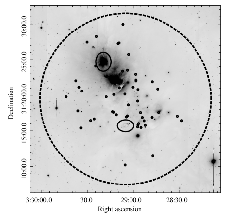
Figure 1.— Subaru/Suprime-Cam i-band image for our target region NGC1333 in the Perseus star forming region. Marked are the cluster radius with a large dashed circle, the two well-known objects BD+30 549 (north) and HH 7-11 (south) with small ellipses, and the population of very low mass members (see this paper, Tables 2 and 4) with small circles. The reflection nebula NGC1333 is slightly north of the image center. Coordinates are J2000. For more information on this image, see Scholz et al. (2009a).

2. Observations and data reduction

Our spectra were obtained with the Fiber Multi Objects Spectrograph (FMOS) at the Subaru Telescope (Kimura et al., 2010) on the night of 2010 November 27. Four-hundred fibers, each of 1.2” diameter are configured by the fiber positioner system of FMOS in the 30’ diameter field of view, with an accuracy of 0.2” rms. The patrol radius of each spine is 87”, while the minimum spacing between two neighboring spines is 12”.

The spectra are extracted by the two spectrographs (IRS1 and IRS2). Our data were obtained in shared-risk mode, using only one of the spectrographs (IRS1, 200 fibers). IRS1 is equipped with a $2048\times 2048$ pixel HAWAII-II HgCdTe detector, and a mask mirror for OH airglow supression. With the low-resolution mode ($R\sim 600$) the spectrograph yields a coverage from 0.9 to 1.8$\,\mu m$ (J- and H-bands). We obtained 10 exposures with 15 min on-source time each.

The observations were carried out in the Normal Beam Switching (NBS) mode, i.e. the same amount of time was spent to observe the sky, which is achieved by offseting the telescope by 10-15”. The seeing during the science observations was stable at $\sim 1$”. Since no stars suitable for telluric correction are found within our science field-of-view, we observed several standard star fields, covering the range of airmasses at which the science target was observed (airmass between 1-2). The observed standard stars have spectral types in the range F4 - G5.

Data reduction was carried out using the data reduction package supplied by the Subaru staff. The package consists of IRAF tasks and C programs using the CFITSIO library. The data reduction package contains the tasks for standard reduction of NIR spectra, performing sky subtraction, bad-pixel and flat-field correction, wavelength calibration, flux calibration and telluric correction. In this last step, each 15-minute exposure was calibrated using a standard star at the appropriate airmass. Finally, the ten individual exposures were averaged. For the analysis (Sect. 3) the spectra were binned to a uniform wavelength interval of 5 Å and smoothed with a small-scale median filter. For the reduced spectra, the signal-to-noise ratio in the H-band ranges from 10 to 70.

In total, we covered 100 targets, from which 71 are selected from our IZ candidate catalogue (Scholz et al., 2009a). 10 additional targets have been selected by combining our JK-catalogue with the ’HREL’ catalogue from the Spitzer ‘Cores to Disk’ (C2D) Legacy program (Evans et al., 2009). All 10 have colour-excess in IRAC bands and thus should have a disk (see Sect. 4.4). 19 fibres were placed on known M-type members for reference (from Wilking et al., 2004; Greissl et al., 2007; Scholz et al., 2009a; Winston et al., 2009).

To test for possible effects of imperfect calibration, we compared the H-band spectra for six objects observed with MOIRCS (Scholz et al., 2009a) and with FMOS (this paper). For three of them there is excellent agreement (SONYC-NGC1333-1, 5, 8), while for the others there are slight differences in the spectral slope. Using the method outlined in Sect. 3.2, we measured the spectral types for the four out of six MOIRCS spectra which cover the entire H-band. All four give types that are later than those derived from FMOS, by 0.4, 1.3, 0.5, 0.7 subtypes, i.e. the differences are larger than our internal accuracy of 0.4 subtypes.

These discrepancies may indicate residual problems with the telluric calibration in the MOIRCS and/or the FMOS data. These problems could be induced by the use of multi-object facilities: Since we stay on the target field for long integration times and the fields themselves do not cover adequate telluric standards, there is a significant time and position offset between science targets and standards, i.e. the depth of the telluric bands could potentially be quite different between science and standard fields.

Stable conditions, as they were present for the FMOS observations, should mitigate this effect. The FMOS data also have the wider wavelength coverage, which facilitates the telluric correction and the spectral analysis. Therefore we put more trust in the quantities derived from FMOS spectra.

3. Spectral analysis

3.1. Selection of young very low mass objects

In total we obtained spectra for 100 objects with FMOS. Based on the broadband spectral shape in the near-infrared, young very low mass sources can be reliably separated from more massive stars. Objects with very low masses and thus effective temperature below $\sim 3500$ K or spectral types of $\sim$M3 or later show broad absorption features of H₂O, which distinguishes them clearly from the smooth near-infrared slopes of more massive and hotter stars (Cushing et al., 2005). The depth of these absorption troughs is a strong function of effective temperature.

The most important spectral feature for our purposes is the H-band ‘peak’, formed by the two H₂O absorption bands at 1.3-1.5 and 1.75-2.05$\,\mu m$. The shape of this feature is gravity sensitive; while it appears round with a flat top in evolved field objects, it is triangular with a pronounced peak at 1.67$\,\mu m$ in young objects with ages of $\lesssim 100$ Myr (Kirkpatrick et al., 2006; Brandeker et al., 2006; Bihain et al., 2010). In addition, H₂O absorption causes a sharp edge at 1.35$\,\mu m$ and another ‘peak’ in the K-band.

We use these features to identify young very low mass sources in the FMOS sample. We are looking for objects showing structure over the full spectral regime, as opposed to a smooth slope. In particular, we select objects with a) a pointy peak in the H-band and b) an absorption edge at 1.35$\,\mu m$. Out of 100 FMOS spectra, 26 show these characteristics and are called YVLM sample (short for ’young very low mass’) in the following. For 11 the spectra are too noisy to make a decision, and the remaining 63 do not show these features. These 63 objects for which we can exclude that they are very low mass sources are listed in Appendix A.

From the 19 literature sources, 16 are re-identified and are part of the YVLM sample. The other 3 have spectra that are too noisy to identify the features. The remaining 10 YVLM objects are newly confirmed very low mass members of NGC1333 and are listed in Table 2. We use the nomenclature SONYC-NGC1333-X for these objects, where X is a running number. Since we have listed objects 1-28 in Scholz et al. (2009a), we continue here with no. 29. Note that the list in Scholz et al. (2009a) contains some previously confirmed members. The spectra for the 10 new objects are shown in Fig. 2. 7 of the new objects come from our IZ catalogue, the remaining 3 from the JK plus Spitzer list (SONYC-NGC1333-31, 32, 33).

Table 2New very low mass members in NGC1333. The IDs SONYC-NGC1333-X are abbreviated with S-X.

ID	$\alpha$(J2000)	$\delta$(J2000)	i’ (mag)	z’ (mag)	J (mag)	K (mag)	$A_{V}$	$A_{V}$	SpT	$T_{\mathrm{eff}}$	Other names
S-29	03 28 28.40	+31 16 27.3	17.637	16.675	14.624	13.624	0	0	M6.9	3150
S-30	03 28 31.08	+31 17 04.1	23.650	21.235	16.823	14.079	9	9	M9.3	2700
S-31	03 29 44.15	+31 19 47.9			17.386	15.290	6	5	$\sim$M9	2300	Sp 132
S-32	03 29 03.21	+31 25 45.2			15.798	13.832	4	4	M7.1	3200	MBO89, Sp 79
S-33	03 29 03.95	+31 23 30.8			17.143	14.932	7	5	M8.3	2500	MBO116, Sp 83
S-34	03 29 06.94	+31 29 57.1	20.839	19.225	16.541	14.774	4	4	M7.0	2950	Sp 90
S-35	03 29 10.18	+31 27 16.0	18.988	17.711	15.547	14.127	2	2	M7.4	3050	MBO94, Sp 96
S-36	03 29 25.84	+31 16 41.8	23.392	21.432	18.53	17.07	2	0	$\sim$L3	2250
S-37	03 29 30.54	+31 27 28.0	17.356	16.344	13.808	12.598	1	2	M6.9	3200	MBO68
S-38	03 29 34.42	+31 15 25.2	21.091	19.654	17.33	16.15	1	1	M7.7	2850

Many of our spectra show emission in Paschen $\beta$ at 1.28$\,\mu m$. If the emission originates from the source itself, it would be a clear indication for ongoing accretion (Natta et al., 2004). However, this is difficult to tell with fibre spectroscopy; our spectra may be affected by emission from the cloud material in NGC1333. Still, it is worth pointing out that the fraction of objects with Pa $\beta$ emission is 50% in the YVLM sample and 32% among the remaining objects. This indicates that the other sources might contain a number of young stars in NGC1333 with temperatures $>3500$ K.

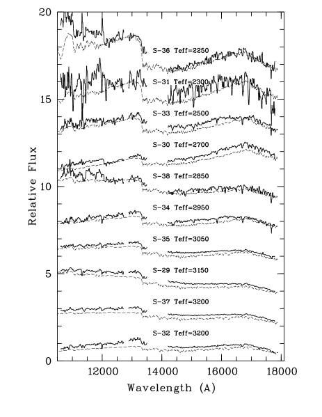
Figure 2.— FMOS spectra for the 10 new brown dwarfs listed in Table 2. The fluxes are on a relative scale with arbitrary offsets. The observed spectrum is shown in black, the best fitting DUSTY model slightly offset, with thin, dashed lines. We masked out the Pa$\beta$ lines for clarity. The identification numbers SONYC-NGC1333-X are abbreviated with S-X.

In Fig. 3 we compare the FMOS spectra for two of our sources, both originally identified in Scholz et al. (2009a), with spectra for young brown dwarfs from Muench et al. (2007, left panel) and old dwarfs with similar spectral types (Burgasser et al., 2008; Burgasser & McElwain, 2006, middle panel). At late M spectral types, the more rounded peak of the old objects becomes visible (compare the young KPNO4 with the old LHS2924). However, for earlier types the difference between young and old is not significant. The plot also illustrates that sufficient signal-to-noise is required to distinguish between the two types of objects. Our spectra often do not have the necessary quality to make this decision. From these arguments it follows that contamination by late M-dwarfs in the field cannot completely be excluded. Given the compact nature of the NGC1333 cluster (see Sect. 4.3) and the low space densities of such objects (Caballero et al., 2008), the contamination is considered to be negligible ($\lesssim 1$).

3.2. Spectral types

Spectral classification for cool dwarfs in the near-infrared relies mostly on the broad H₂O absorption features mentioned above. A number of spectral indices has been suggested in the literature. Relevant for us are the indices that are calibrated for young brown dwarfs and thus take into account the fact that the absorption features are sensitive to gravity. Such indices have been proposed by Wilking et al. (2004), Allers et al. (2007), and Weights et al. (2009). We find, however, that these schemes are of limited use for our low-resolution and (mostly) low signal-to-noise spectra, mainly because the wavelength offset between the two intervals from which the index is derived is relatively small, e.g. 0.058$\,\mu m$ for the H₂O index (Allers et al., 2007) or 0.103$\,\mu m$ for the WH index (Weights et al., 2009).

For our purposes we require a flux ratio that maximises the contrast between the numerator and the denominator. This is achieved by using the flux ratio between 1.675-1.685$\,\mu m$ and 1.495-1.505$\,\mu m$. The first interval is chosen because it corresponds to the position of the H-band peak for young objects with M6-M9 spectral type. The second interval marks the lowest flux level on the blue side of the H-band peak for such objects.

Table 3Objects used to calibrate the H-peak index.

Name	SpT	J (mag)	K (mag)	$A_{V}$ (mag)	HPI
ITG2	M7.25	11.540	10.097	2.40	1.050
J0444	M7.25	12.195	10.761	2.35	1.124
CFHT6	M7.5	12.646	11.368	1.51	1.135
KPNO2	M7.5	13.925	12.753	0.93	1.136
KPNO5	M7.5	12.640	11.536	0.56	1.137
CFGH3	M7.75	13.724	12.367	1.94	1.184
J0441	M7.75	13.730	12.220	2.77	1.098
CFHT4	M7.0	12.168	10.332	4.53	1.009
MHO4	M7.0	11.653	10.567	0.47	1.174
KPNO7	M8.25	14.521	13.271	1.37	1.121
KPNO1	M8.5	15.101	13.772	1.78	1.203
KPNO6	M8.5	14.995	13.689	1.63	1.185
KPNO9	M8.5	15.497	14.185	1.69	1.155
LRL405	M8.0	15.28	13.91	2.01	1.126
J0457	M9.25	15.771	14.484	1.56	1.240
KPNO4	M9.5	14.997	13.281	3.91	1.342
KPNO12	M9.0	16.305	14.927	2.01	1.261
J1207	M8.0	12.995	11.945	0.81	1.226
J1139	M9.0	12.686	11.503	0.99	1.336
J1245	M9.5	14.518	13.369	0.81	1.306

This index, dubbed HPI for H-peak index, is illustrated in the left and middle panel of Fig. 3 where we show literature spectra for young and old brown dwarfs in Taurus with spectral types M7 and M9.5 compared with FMOS data for two of the brown dwarfs in NGC1333. The H-band peak clearly is highly sensitive to the spectral type in this regime. We expect that this index increases from mid M to late M spectral types. The figure also demonstrates the advantages of this index at low signal-to-noise ratio.

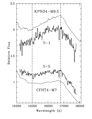
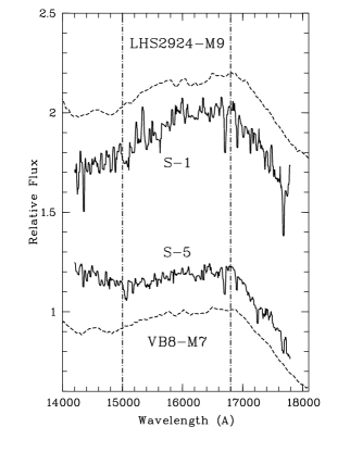
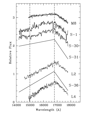
Figure 3.— Dereddened spectra of SONYC objects in NGC1333 (solid lines) compared with different comparison spectra (dashed lines). Spectra are offset by a constant value for clarity. The spectral range for the HPI is indicated with dashed lines. The SONYC-NGC1333-X identification numbers are abbreviated with S-X in all three panels. Left panel: Young brown dwarfs in Taurus (Muench et al., 2007). Middle panel: M dwarf spectral standards in the field (Burgasser et al., 2008; Burgasser & McElwain, 2006). Right panel: Young substellar companions (M8 - HIP78530B (Lafrenière et al., 2011), L2 - 2M1207B (Patience et al., 2010), L4 - 1RXSJ1609-2105B (Lafrenière et al., 2010). In the right panel, we approximate the spectral slope for two of the faintest objects with a linear fit, the full spectra are shown in Fig. 2.

To calibrate the HPI, we use literature spectra for 20 young brown dwarfs with spectral types M7-M9.5, for which spectra are publicly available in the SpeX Prism Spectral Libraries (Muench et al., 2007; Looper et al., 2007). Their spectra have been dereddened using the reddening law $A_{\lambda}=(\lambda/1.235\,\mu m)^{-1.61}\cdot A_{J}$ and the relation $A_{J}=0.3088\cdot A_{V}$. The optical extinction $A_{V}$ is derived from their $J-K$ colours:

$$A_{V}=[(J-K)-(J-K)_{0}]/0.1844$$ (1)

These relations are based on the extinction law from Cardelli et al. (1989) for $R_{V}=4.0$, which is used throughout this paper. We note that $R_{V}$ varies within star forming regions typically from 3 to 5; the adopted value is an average from the values measured by Cardelli et al. (1989) for diffuse and dense regions of the interstellar medium. It is also a reasonable average for our target region NGC1333 (Cernis, 1990).

For the reasons outlined in Scholz et al. (2009a) we use $(J-K)_{0}=1.0$. The resulting uncertainty in $A_{V}$ is $\sim 1$ mag. For example it is possible that we overestimate $A_{V}$ due to the presence of K-band excess from a disk. This induces an uncertainty of up to 0.04 in the HPI. Note that the literature spectral types for the calibrators have been determined in the optical by comparison with templates (e.g. Briceño et al., 2002). The internal accuracy of these optical types is typically $\pm 0.25$ subtypes. The calibrators are listed in Table 3.

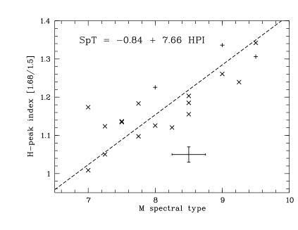
Figure 4.— H-peak index (HPI) calculated as flux ratio between 1.675-1.685$\,\mu m$ and 1.495-1.505$\,\mu m$ plotted vs. (optical) spectral type for published spectra from Muench et al. (crosses, 2007) and Looper et al. (plusses, 2007). The correlation after excluding the outlier MHO4 at M7 is $\mathrm{SpT}=-0.84+7.66\cdot\mathrm{HPI}$ (dashed line). A typical errorbar is overplotted.

In Fig. 4 we plot the HPI for the 20 calibrators. The plot shows the expected correlation between index and spectral type. The one outlier at spectral type M7 corresponds to the object MHO4 and deviates in its HPI by $3\sigma$ from a linear fit. Nothing particular can be seen in its spectrum which would explain this discrepancy. Based on the H-band peak, MHO4 appears to have a later spectral type than indicated in the literature. Excluding MHO4, we derive a correlation of

$$\mathrm{SpT}=-0.84+7.66\cdot\mathrm{HPI}$$ (2)

with an 1$\sigma$ scatter of 0.37 subclasses. The 1$\sigma$ scatter in HPI around the correlation is 0.039. As outlined above, this can be attributed to the uncertainty in the extinction. The HPI is properly calibrated for types M7-M9.5, but may also hold for later spectral types as the H-band peak increases in strength in the L-type regime (see below).

We note that this correlation does not hold for field dwarfs. As seen in the middle panel of Fig. 3 these objects have flatter H-band peaks which results in lower values for the HPI for a given spectral type.

Using this index we determined spectral types for all 26 objects in the YVLM sample, after dereddening using the corrected extinction derived in Sect. 3.3. 9 of them have published spectral types. Five of them (MBO69, MBO54, MBO77, ASR29, ASR83) are based on an index defined in the K-band (Wilking et al., 2004; Greissl et al., 2007). The other four have the Spitzer IDs 131, 104, 118, and 46 in Winston et al. (2009) and were classified in the optical. Excluding MBO54, ASR29, Sp 104 and Sp 118 which have a published spectral type of M6 or earlier, for which the HPI is not properly calibrated, the HPI types deviate by -0.4, -0.2, -0.2, -0.1, +0.6 subtypes from the published ones, which provides some reassurance in the usefulness of the HPI. The 10 new objects have spectral types of M6.9 or later, classifying them as likely brown dwarfs. The spectral types for the new and known sources are listed in Table 2 and 4 respectively.

In the right panel of Fig. 3 we compare FMOS data for the four latest-type SONYC objects with spectra for young ultracool objects with published spectral types: the M8 companion to HIP78530 (Lafrenière et al., 2011), the L2 companion to the TW Hya brown dwarf 2M1207 (Patience et al., 2010), and the L4 companion to 1RXSJ1609-2105B (Lafrenière et al., 2010), all three with ages of 5-10 Myr. Using the HPI, we get spectral types of M8, L2, and L3.5 for these three comparison objects, consistent with the literature values, which indicates that HPI could be useful for spectral typing of young early L-dwarfs as well. In this plot we approximate the spectral slopes for the two faintest objects in our sample with linear fits on either side of the H-band peak, to facilitate the comparison. The plot demonstrates that objects SONYC-NGC1333-1, 30, 31 are about or later than M8 and clearly earlier than L2, in line with our classification. The object SONYC-NGC1333-36 compares well with the L2 and L4 templates, which makes it the coolest object discovered in NGC1333 so far.

We note that the redward slope of the H-band peak appears anomalously steep for SONYC-NGC1333-31 and 36. This is not introduced by the linear fit or the treatment of the spectra, and it is not seen in the other FMOS spectra for NGC1333 or $\rho$ Oph (Muzic et al., subm.), which makes a calibration problem unlikely. The effect is difficult to explain, as these two spectra are very noisy, but it could in principle be a real feature, especially since the data is well-matched by the model spectrum (see Sect. 3.3). Better quality spectra are needed to verify the parameters for these objects. Since the HPI is defined for the blueward slope of the H-band peak, this does not affect the spectral typing.

3.3. Model fitting

For the 26 objects in the YVLM sample the FMOS spectra were compared with AMES-DUSTY models (Allard et al., 2001) for low gravity ($\log{g}=3.5$ or, if not available, $4.0$) low-mass stars. Using the extinction law described in Sect. 3.2 we calculated a model grid for $T_{\mathrm{eff}}=1500$ to 3900 K in steps of 100 K and $A_{V}=1$ to 20 mag in steps of 1 mag. The models were binned to 5 Å, the same binsize as the FMOS data.

The fitting was done in a semi-interactive way. Since extinction and effective temperature cannot be determined separately with low-resolution, low signal-to-noise spectra, we started by adopting the $A_{V}$ determined from the $J-K$ colour, using Equ. (1). For each of the YVLM objects, we calculated the following test quantity ($O$ - observed flux; $M$ - model flux; $N$ - number of datapoints):

$$\chi=\frac{1}{N}\sum_{i=1}^{N}\frac{(O-M)^{2}}{M}$$ (3)

This was done for the series of models using the ’photometric’ $A_{V}$; we selected the one with the minimum $\chi$, which is typically between 0.005 and 0.05 (with one exception with 0.2). This means that the average deviation between observed and model spectrum in a given wavelength bin of 5 Å is in the same range as the noise in the observations.

Usually a few model spectra (2-4) give indistinguishable $\chi$; we adopt the average $T_{\mathrm{eff}}$ from these best fitting models. A visual inspection of the observed spectra with models for a range of temperatures shows that clear discrepancies are visible for temperatures which are $>200$ K different from the adopted value, i.e. the uncertainty in the adopted values is $\pm 200$ K. We note that effective temperatures are necessarily model dependent; our values should only be interpreted in the context of the AMES-DUSTY models. The best fitting models are plotted as thin, dashed lines in Fig. 2 for the 10 newly identified objects.

In 6/10 cases this initial fit is already convincing. In two more cases, it can be improved by slightly adjusting $A_{V}$ by 1 mag, which is within the uncertainty for $A_{V}$ (see Sect. 3.2). The two remaining cases give the best fit when $A_{V}$ is changed by 2 mag compared with the initial estimate. In Table 2 we list the photometric and adjusted value for $A_{V}$ and the best fit value for the effective temperature.

For SONYC-NGC1333-36, the coolest object in our sample, we find an effective temperature of 2250 K, which is significantly higher than the published values for the two comparison objects shown in Fig. 3 (right panel). For 1RXSJ1609-2105B Lafrenière et al. (2010) find $1800\pm 200$ K based on DUSTY and Drift-Phoenix (Helling et al., 2008) models. For 2M1207B, two independent groups determined $1600\pm 100$ K, again based on comparison with DUSTY spectra (Patience et al., 2010; Mohanty et al., 2007), although Skemer et al. (2011) suggest that the actual value might be as low as 1000 K. The DUSTY spectra for $<2000$ K are clearly not in agreement with our spectrum for SONYC-NGC1333-36. One possible explanation is that model fitting for the comparison objects has been done over the full near-infrared range, whereas in our case $T_{\mathrm{eff}}$ is mostly fixed by the shape of the H-band peak. We will revisit this issue in Sect. 3.4.

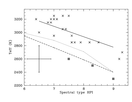
Figure 5.— Comparison between the spectral types and effective temperatures for the YVLM sample, as determined in this paper (Sect. 3.2 and 3.3). A typical errorbar is overplotted. The solid line is a linear fit to the datapoints excluding the 3 outliers marked with squares. We also show the effective temperature scales by Mentuch et al. (2008, dashed line) and Luhman et al. (2003, dotted line).

In Fig. 5 we compare the derived effective temperatures with the spectral types determined with the HPI in Sect. 3.2. The expected trend – cooler temperatures correspond to later spectral types – is visible, with only three exceptions. For two of these exceptions (SONYC-NGC1333-17 and -31), the signal-to-noise ratio in the spectrum is very poor ($\sim 10$), i.e. the uncertainties in spectral type and temperature are large. For SONYC-NGC1333-17 there are two published spectral types of M8 and M8.7, which would move the datapoint closer to the general trend. The third outlier (SONYC-NGC1333-33) has an unusual dip in the spectrum around 1.65$\,\mu m$, which decreases our spectral type estimate by $\sim 1$ subtype, but does not affect the model fitting. Excluding these three outliers, the datapoints are well-approximated by a linear trend (solid line): $T_{\mathrm{eff}}=4191-157\times\mathrm{SpT}$ (where SpT corresponds to the M subtype).

The plot also shows the effective temperature scales by Mentuch et al. (2008, dashed line) and Luhman et al. (2003, dotted line), which are derived using the optical portion of the spectrum. The two scales agree fairly well with each other, although the Mentuch et al. scale is an extrapolation and has not been directly calibrated for $T_{\mathrm{eff}}<3000$ K. The trend seen in our data is consistent with these lines. Our datapoints are, however, mostly above the two lines, indicating that we systematically overestimate the temperatures (by $\sim 200$ K) or the spectral types (by 0.5-1 subtypes).

We explored possible reasons for this discrepancy. One option is a systematic error in the extinction. Decreasing $A_{V}$ by 1 mag for all objects would shift their spectral types to earlier types, but only by $\sim 0.3$ subtypes, not sufficient to explain the effect. Moreover, this would also increase the best estimate for $T_{\mathrm{eff}}$ by typically 200 K and thus cause larger disagreement between datapoints and published effective temperature scales. The inverse is true as well – increasing $A_{V}$ would lead to lower $T_{\mathrm{eff}}$, as required, but also to later spectral types. Thus, systematic changes in $A_{V}$ do not resolve the problem. Given the good agreement between our spectral types and literature values (Sect. 3.2), we suspect that the offset is most likely due to a problem with the effective temperatures and could indicate issues with the used model spectra. A more extensive comparison of the effective temperature scales is beyond the scope of this paper.

3.4. Spectral flux distributions

To further test the spectral fitting from Sect. 3.3 we compare the full photometric spectral flux distributions (SFD) for some selected sources, as far as available, with the AMES-DUSTY model spectra. We include our own photometry in izJK as well as Spitzer/IRAC data from the C2D ’HREL’ catalogue (Evans et al., 2009). In Fig. 6 we show 3 examples.

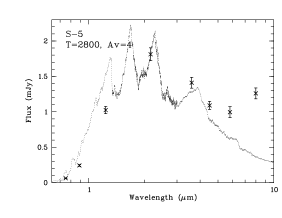
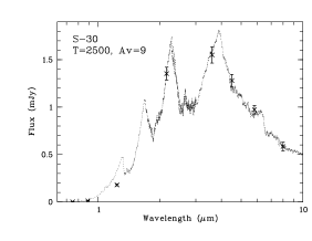
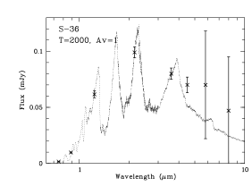
Figure 6.— Photometric spectral flux distributions for three of the coolest members in NGC1333 in comparison with AMES-DUSTY model spectra. The disk excess for SONYC-NGC1333-5 is clearly visible. The SONYC-NGC1333-X identification numbers are abbreviated with S-X in all three panels. Errorbars for the fluxes are overplotted, but they are too small to be visible in some of the blue bands.

Object SONYC-NGC1333-5 is well-matched by a model spectrum for $T_{\mathrm{eff}}$ of 2800-2900 K for $A_{V}=4$ mag, in line with the parameters derived from the FMOS spectrum (Table 4). This object shows colour excess redwards of 5$\,\mu m$, presumably due to the presence of a disk (see Sect. 4.4). The best match for object SONYC-NGC1333-30 is obtained for $T_{\mathrm{eff}}$ of 2500-2700 with $A_{V}$ of 9-10 mag, i.e. the object may be slightly cooler than listed in Table 2, but still within the uncertainty. For the coolest object SONYC-NGC1333-36 a good match is found for temperatures between 1900 and 2100 K and $A_{V}$ of 0-2 mag. This is again somewhat cooler than the estimate given in Table 2.

In general, when comparing with the full SFD the results are similar to the spectral fits to individual wavelength bands in the near-infrared, maybe except for the regime below 2500 K where the SFD comparison yields lower temperatures by $\sim 200$ K. The comparison also illustrates that the ideal dataset for a characterisation of young brown dwarfs would be a spectrum covering the entire near-infrared domain from 1 to 8$\,\mu m$, thus including five broadband features.

4. The brown dwarf population in NGC1333

The newly identified very low mass objects in this paper add to the substantial number in the NGC1333 region that have already been confirmed in the literature. In Table 4 we compile all previously spectroscopically confirmed objects with spectral types of M5 or later or effective temperatures of 3200 K or below, from Scholz et al. (2009a), Wilking et al. (2004), Greissl et al. (2007), and Winston et al. (2009). Whenever possible, we also re-measured the HPI spectral types for the sources identified in Scholz et al. (2009a), based on their MOIRCS spectra. In the Table, we list coordinates, photometry, spectral types, effective temperatures, and alternative names. Adding the 10 objects discovered in this paper, the entire sample comprises 51 objects.

Not all these objects are brown dwarfs; some are very low mass stars. Based on the COND, DUSTY, and BCAH isochrones (Baraffe et al., 2003; Chabrier et al., 2000; Baraffe et al., 1998), the hydrogen burning limit at 1 Myr would be reached at effective temperatures of 2800-2900 K, which is found to correspond to an (optical) spectral type of M6-M7 (Luhman et al., 2003; Mentuch et al., 2008). In Table 4 we made the cut at M5 to include all borderline cases as well. Taking this into account, the number of confirmed brown dwarfs in NGC1333 is about $35\pm 5$. This is currently one of the largest and best characterised populations of substellar objects in a single star forming region. In the following we will investigate the mass function, spatial distribution, and disk properties for this sample.

Table 4Previously confirmed very low mass members in NGC1333. The IDs SONYC-NGC1333-X are abbreviated with S-X.

ID	$\alpha$(J2000)	$\delta$(J2000)	J (mag)	K (mag)	SpT	$T_{\mathrm{eff}}$	Other names
S-1	03 28 47.66	+31 21 54.6	17.55	15.24	M9.2a	2600a, 2800b	MBO139
S-2	03 28 54.92	+31 15 29.0	15.990	14.219	M7.9a, M6.5b, M8d, M8.6f	2850a, 2600b	ASR109, Sp 60
S-3	03 28 55.24	+31 17 35.4	15.090	13.433	M7.9c, M8.2f	2900b	ASR38
S-4	03 28 56.50	+31 16 03.1	18.17	16.73	M9.6f	2500b
S-5	03 28 56.94	+31 20 48.7	15.362	13.815	M7.6a, M6b, M6.8c	2850a, 2900b	MBO91, Sp 66
S-6	03 28 57.11	+31 19 12.0	17.24	15.34	M7.3a, M8b, M8.0f	3250a, 2700b	MBO148, ASR64, Sp 23
S-7	03 28 58.42	+31 22 56.7	15.399	13.685	M6.5b, M7.1c, M7.7f	2800b	MBO80, Sp 72
S-8	03 29 03.39	+31 18 39.9	15.833	14.000	M8.2a, M8.5b, M7.4c, M8.4f	2850a, 2600b	MBO88, ASR63, Sp 80
S-9	03 29 05.54	+31 10 14.2	17.072	15.667	M8b, M8.6f	2600b
S-10	03 29 05.66	+31 20 10.7	17.113	15.485		2500b	MBO143, Sp 86
S-11	03 29 07.17	+31 23 22.9	17.87	15.62	M9.2f	(2600)b	MBO141
S-12	03 29 09.33	+31 21 04.2	16.416	13.150		(2500)b	MBO70, Sp 93
S-13	03 29 10.79	+31 22 30.1	14.896	12.928	M7.5b, M7.4c, M8.1f	3000b	MBO62
S-14	03 29 14.43	+31 22 36.2	14.606	13.035	M7b, M6.6c, M7.7f	2900b	MBO66
S-15	03 29 17.76	+31 19 48.1	14.803	12.988	M7.5b, M6.5c, M7.8f	3000b	MBO64, ASR80, Sp 112
S-16	03 29 28.15	+31 16 28.5	13.054	12.091	M8.5a, M7.5b, M7.5e, M9.1f	2850a, 2600b, 2761e	Sp 164
S-17	03 29 33.87	+31 20 36.2	16.562	15.481	M7.5a, M8b, M8.7f	2600a, 2500b	MBO140
S-18	03 29 35.71	+31 21 08.5	18.50	16.94	M8.2f	2500b	Sp 129
S-19	03 29 36.36	+31 17 49.8	17.91	16.38		2700b
S-21	03 28 47.34	+31 11 29.8	15.484	12.702		3100b	ASR117
ASR15	03 28 56.94	+31 15 50.3	15.056	13.461	M7.4c, M6.0d
ASR17	03 28 57.15	+31 15 34.5	15.405	13.186	M7.4c, M6.0d		Sp 68
MBO73	03 28 58.24	+31 22 09.3	16.004	13.367	M6.4c		Sp 70
ASR24	03 29 11.30	+31 17 17.5	13.977	12.915	M8.2c, M8.0d
MBO69	03 29 24.45	+31 28 14.9	14.041	12.686	M7.0a, M7.4c	3200a
ASR29	03 29 13.61	+31 17 43.4	16.441	13.028	M5d	3250a
ASR105	03 29 04.66	+31 16 59.1	15.550	12.665	M6d		Sp 84
ASR8	03 29 04.06	+31 17 07.5	13.310	12.313	M7d
MBO78	03 29 00.15	+31 21 09.2	16.466	13.349	M5d		Sp 75
Sp 45	03 28 43.55	+31 17 36.4	12.219	10.138	M5.0e	3125e	ASR127
Sp 46	03 28 44.07	+31 20 52.8	14.245	12.627	M7.3a, M7.5e	3050a, 2829e
Sp 49	03 28 47.82	+31 16 55.2	12.940	10.909	M8.0e	2710e	ASR111
Sp 53	03 28 52.13	+31 15 47.1	13.161	12.029	M7.0e	2846e	ASR45
Sp 55	03 28 52.90	+31 16 26.4	13.616	12.476	M5.0e	3154e	ASR46
Sp 58	03 28 54.07	+31 16 54.3	13.027	11.599	M5.0e	3098e	ASR42
Sp 94	03 29 09.48	+31 27 20.9	14.154	12.692	M5.0e	3098e	MBO60
Sp 105	03 29 13.03	+31 17 38.3	15.231	14.158	M8.0e	2710e	ASR28
Sp 131	03 29 37.73	+31 22 02.4	13.987	12.958	M7.6a, M7.0e	2850a, 2891e	MBO65
Sp 157	03 29 12.79	+31 20 07.7	14.676	13.294	M7.6a, M7.7c, M7.5e	2950a, 2812e	MBO75, ASR83
Sp 177	03 29 24.83	+31 24 06.2	14.433	13.383	M6.5a, M6.7c, M6.5e	3000a, 2957e	MBO77
Sp 71	03 28 58.24	+31 22 02.1	14.912	12.406	M6e	2990e	MBO47

4.1. The number of brown dwarfs

Based on our comprehensive spectroscopy, we can put some constraints on the total number of brown dwarfs in NGC1333 and the mass limits of the current surveys. For this purpose, we use the iz survey presented in Scholz et al. (2009a). In Fig. 7 we plot the iz colour-magnitude diagram for the 196 candidates selected in Scholz et al. (2009a). The confirmed brown dwarfs (Tables 2 and 4), either by us or other groups, are marked with squares; all objects for which we have obtained spectroscopy with crosses. Note that the iz candidates are selected only with a cut in colour and a cut in PSF shape to rule out extended objects. No other selection criteria have been used, i.e. this sample is as unbiased as possible.

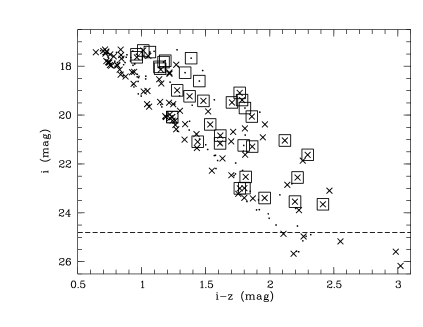
Figure 7.— Colour-magnitude diagram for the iz candidates (dots), originally identified in Scholz et al. (2009a). Crosses are objects for which we have obtained spectra in this paper or Scholz et al. (2009a). Confirmed very low mass objects from this paper or the literature are marked with squares. The horizontal dashed line shows the completeness limit of the survey estimated in Scholz et al. (2009a).

We have useful spectra for 98/196 candidates; out of these 98, 24 are confirmed by our spectra. In total the iz sample contains 35 confirmed objects with $A_{V}\lesssim 12$ mag. Thus, we have a yield of 24/98 (24%) and would expect to find 24 more objects among the candidates for which we do not have spectra. Since 11 of them (35 minus 24) have already been confirmed by other groups, the expected number of additional very low mass objects from this iz selection is 13.

The low-mass end of the diagram deserves additional discussion. The faintest confirmed brown dwarfs in Fig. 7 are SONYC-NGC1333-1, 30, and 36 at $i=23.4-23.7$. Comparing their effective temperatures with the 1 Myr DUSTY and COND isochrones, it seems likely that they have masses of $\lesssim 0.02\,M_{\odot}$. If our estimate of $T_{\mathrm{eff}}=2000$ K for SONYC-NGC1333-36 is correct (Sect. 3.4), the best mass estimate would be in the range of 0.006$\,M_{\odot}$.

We have taken spectra for 7 fainter objects, but none of them is a brown dwarf, which might indicate that we have reached the ’bottom of the IMF’, as preliminarily stated in Scholz et al. (2009a). However we may not be 100% complete in this magnitude range. The formal completeness limits of the iz survey at $i=24.8$ mag, determined from the peak of the histogram of the magnitudes (see Scholz et al., 2009a), is shown with a dashed line. This limit has been derived for a field of view of $34^{\prime}\times 27^{\prime}$, but most of the cluster members are located in a smaller region of $10^{\prime}\times 10^{\prime}$ which is partially affected by significant background emission from the cloud (see Fig. 1. Thus, the completeness limit in the relevant areas might not always reach the value shown in Fig. 7.

Thus, based on our new data we retract the previous claim by Scholz et al. (2009a) stating a deficit of objects with $M<0.02\,M_{\odot}$ in NGC1333, for two reasons: a) The updated brown dwarf census contains a few of objects with masses at or below 0.02$\,M_{\odot}$, including one with an estimated mass of 0.006$\,M{\odot}$. b) The current survey may not be complete at the lowest masses, i.e. we cannot exclude the presence of a few more objects with $M<0.02\,M_{\odot}$.

The census for $M>0.02\,M_{\odot}$ is more robust. From the 35 confirmed members in the iz diagram we subtract 10 which are probably slightly above the substellar boundary (see discussion in Sect. 4). We also subtract the 3 which are likely below $0.02\,M_{\odot}$ and add the 13 which we are still missing. This gives a total number of $\sim 35$ brown dwarfs down to $0.02\,M_{\odot}$ and with $A_{V}\lesssim 12$ mag.

4.2. The star vs. brown dwarf ratio

As a proxy for the shape of the mass function, previous authors have used the ratio of stars to brown dwarfs, where these two groups are defined by a range of masses. These ratios are more robust against uncertainties in the masses than a complete IMF. Andersen et al. (2008) use a range of 0.08-1.0$\,M_{\odot}$ for stars and 0.03-0.08$\,M_{\odot}$ for brown dwarfs, hereafter called $R_{1}$. Other authors use 0.08-10$\,M_{\odot}$ for stars and 0.02-0.08$\,M_{\odot}$ for brown dwarfs, hereafter called $R_{2}$ (e.g. Briceño et al., 2002; Muench et al., 2002; Luhman et al., 2003). Since the number of high-mass stars is small, the two ratios $R_{1}$ and $R_{2}$ should be fairly similar.

The comparison with NGC1333 is complicated by the fact that no comprehensive spectroscopic census is available for the stars. The best starting point is probably the Spitzer analysis by Gutermuth et al. (2008). They find a total of 137 Class I and II members with disk, from which 94 are in 2MASS. Objects not detected in 2MASS are likely embedded sources with high extinction $A_{V}>10$ mag and thus not comparable with our brown dwarf sample. We calculated absolute J-band magnitudes for this sample using the dereddening described in Sect. 3.2 and assuming a distance of 300 pc, which gives a range of $M_{J}=0-9$ mag. Comparing with the BCAH 1 Myr isochrone (Baraffe et al., 1998) the sample contains 13 objects with $M>1.0\,M_{\odot}$, 52 objects with $0.08<M<1.0\,M_{\odot}$ and 29 with $0.02<M<0.08\,M_{\odot}$. These are only objects with disks; correcting for a disk fracton of 83% (Gutermuth et al., 2008) shifts the numbers to 16, 63, 35. The latter number is consistent with the estimate of brown dwarfs in this cluster given in Sect. 4.1. Out of 35 brown dwarfs, the number of objects with masses above 0.03$\,M_{\odot}$ would be 28.

Based on these estimates the ratios for NGC1333 become $R_{1}=63/28=2.3\pm 0.5$ and $R_{2}=79/35=2.3\pm 0.5$ (see below for an explanation of the uncertainties). Our value for $R_{1}$ is somewhat larger than our first estimate given in Scholz et al. (2009a) of $1.5\pm 0.3$, mainly because we use here the cutoff at 0.03$\,M_{\odot}$ to be consistent with Andersen et al. (2008).

The uncertainties for $R_{1}$ and $R_{2}$ stated above are 1$\sigma$ confidence intervals and have been derived based on the prescription provided by Cameron (2011). This prescription is given for population proportions (’success counts’). Therefore, we use the Cameron equation to calculate the confidence intervals $\sigma_{k1}$ for the ratio of number of stars to the sum of stars and brown dwarfs ($k1$) and $\sigma_{k2}$ for the ratio of number of brown dwarfs to the same sum ($k2$). The confidence intervals for $R_{1}$ and $R_{2}$ are then derived as follows:

$$R_{\mathrm{max}}=\frac{k1+\sigma_{k1}}{k2-\sigma_{k2}}$$ (4)

$$R_{\mathrm{min}}=\frac{k1-\sigma_{k1}}{k2+\sigma_{k2}}$$ (5)

Table 5Star to brown dwarf ratios for various star forming regions (see text)

Region	$R_{1}$	$R_{2}$
NGC1333	2.3 (1.8-2.8)	2.3 (1.8-2.7)
ONC	3.3 (2.8-3.9)	3.8,4.5,5.0
UpSco	3.8 (3.1-4.5)	–
NGC2024	3.8 (2.6-5.2)	–
Chamaeleon	4.0 (2.3-6.0)	3.9 (2.9-5.0)
$\rho$-Oph	5.1 (3.8-6.4)	4.8 (3.7-6.0)
Taurus	6.0 (4.5-7.7)	7.3 (5.1-9.6)
IC348	8.3 (6.4-10.5)	8.0 (6.3-10.0)

In Table 5 we compare the ratios for NGC1333 with the available literature values for $R_{1}$ and $R_{2}$ for other regions. The same numbers are plotted in Fig. 8 for illustration. To have accurate and consistent confidence intervals, we re-calculated the errors for all literature values as described above. NGC1333 has the lowest ratios measured so far in any star forming region, suggesting that the number of brown dwarfs in NGC1333 is unusually high, which is in line with the conclusion in Scholz et al. (2009a). In particular, the ratios for NGC1333 deviate by more than 2$\sigma$ from those in IC348. It should be noted that the current census for IC348 (Luhman et al., 2003) is nearly complete down to 0.03$\,M_{\odot}$ and covers most of the cluster, which makes the difference to NGC1333 even more striking.

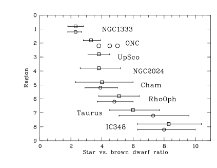
Figure 8.— Star vs. brown dwarf ratios for various star forming regions, from Table 5. $R_{1}$ is plotted with squares, $R_{2}$ with circles. The number on the y-axis is identical with the row in Table 5.

This finding has to be substantiated with further survey work in diverse regions. In Table 5 we list the statistical 1$\sigma$ confidence intervals, purely based on the sample sizes. These statistical errors do not take into account additional sources of uncertainty, e.g. unrecognised biases, inconsistencies in sample selection or problems with the mass estimates, i.e. the actual errors may be larger than listed in Table 5. In particular, it is important to note that all mass estimates are necessarily model-dependent. For the value in NGC1333 we use the BCAH isochrones, mainly because they cover the brown dwarf regime down to the Deuterium burning limit. The problems and uncertainties of these type of models at very young ages are well-documented (Baraffe et al., 2002).

The best way of assessing the overall uncertainties is to compare results from independent surveys. As can be seen in Table 5, so far the results from independent groups agree within the statistical errorbars, with the possible exception of the ONC. Such an independent confirmation is required for NGC1333 as well.

If confirmed, the unusually low ratio of stars to brown dwarfs in NGC1333 could point to regional differences in this quantity, possibly indicating environmental differences in the formation of very low mass objects. One option to explain this is turbulence, as very low mass cores which can potentially collapse to brown dwarfs could be assembled by the turbulent flow in a molecular cloud (Padoan & Nordlund, 2004). At first glance this could be a realistic possibility for NGC1333, where the cloud is strongly affected by numerous outflows (Quillen et al., 2005), although it is not clear if the turbulence in NGC1333 is mainly driven by these outflows (Padoan et al., 2009). Alternatively, additional brown dwarfs could form by gravitational fragmentation of gas falling into the cluster center (Bonnell et al., 2008). This latter mechanism would benefit from the fact that NGC1333 has a higher stellar density and thus a stronger cluster potential than most other nearby star forming regions (Scholz et al., 2009a).

4.3. Spatial distribution

In Fig. 9 we show the spatial distribution of the sample of very low mass objects listed in Tables 2 and 4 (squares). For comparison, the positions of the 137 Class I and Class II sources (Gutermuth et al., 2008) are overplotted with crosses. The dots indicate the positions of all targets for which we have obtained spectra but which are not confirmed as very low mass objects. Additionally, we show the frequency of objects as a function of distance from the cluster center in Fig. 10, again for the same three samples, and in addition for all photometric candidates from our iz catalogue (dash-dotted line).

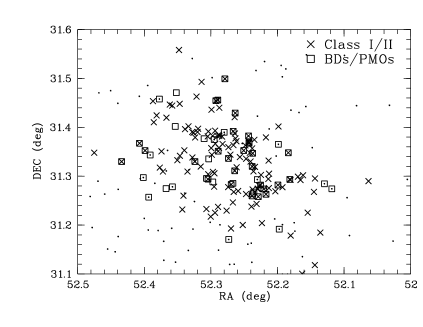
Figure 9.— Spatial distribution of NGC1333 members. Crosses are all 137 objects with Spitzer excess by Gutermuth et al. (2008), squares are all confirmed brown dwarfs (Tables 2 and 4). Objects with spectroscopy for which we can exclude that they are substellar members are shown with dots.

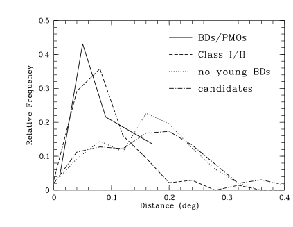
Figure 10.— Histogram of the distance from the cluster center for confirmed brown dwarfs (solid line, Tables 2 and 4), objects with Spitzer excess by Gutermuth et al. (2008) (dashed line), objects for which we can exclude that they are substellar members (dotted line), and all IZ candidates (dash-dotted line). As cluster center we used the average position of the Class I/II sources.

In the two figures, the spatial distribution of brown dwarfs is strongly clustered and indistinguishable from the distribution of the total population of Class I/II sources in NGC1333. For the two samples, the average $\alpha$ and $\delta$ differ only by 0.4’ and 0.3’, respectively, which is $<10$% of the cluster radius. Adopting the average position of the Class I/II sources as cluster center, the average distance from the center is similar in the two samples, 5.2’ for the very low mass objects and 5.5’ for the Class I/II sources. The fraction of objects with distance from the cluster center of $d<0.1$, $0.1<d<0.2$, $d>0.2$ deg is 65, 35, 0% for the very low mass objects and 67, 26, 6% for the Class I/II objects. The scatter in the positions is $\sigma_{\alpha}=0.071$ and $\sigma_{\delta}=0.069$ deg for the very low mass objects, and $\sigma_{\alpha}=0.067$ and $\sigma_{\delta}=0.085$ deg for the Class I/II sources. For all these quantities there are no significant differences between the two samples.

The figures also show that our spectroscopic follow-up covers an area that is about 1.5-2 as large (in radius) than the cluster itself. We took spectra for 31 candidates with distances of $>0.2$ deg from the cluster center, but none of them turned out to be a brown dwarf. There are still 43 candidates from the IZ photometry outside 0.2 deg (see Sect. 4.1) for which we do not have spectra, but based on our current results, it is unlikely that they contain any very low mass cluster members. Thus, our wide-field follow-up spectroscopy shows that there is no significant population of brown dwarfs at $d>0.2$ deg from the cluster center, corresponding to $\sim 1$ pc at a distance of 300 pc.

It has been suggested that gravitational ejection occurs at an early stage in the evolution of substellar objects, either from multiple stellar/substellar systems (Reipurth & Clarke, 2001; Umbreit et al., 2005) or from a protoplanetary disk (Stamatellos & Whitworth, 2009). This ejection is thought to remove the objects from their accretion reservoir and thus sets their masses. In these scenarios one could expect the brown dwarfs to have high spatial velocities in random directions.

An ejection velocity of 1 kms^-1 would allow the object to travel 1 pc in 1 Myr, i.e. in the case of NGC1333 this would be sufficient to reach the edge of the cluster. However, the gravitational potential of the cluster will significantly brake the motion of the brown dwarf. Assuming a total cluster mass of 500$\,M_{\odot}$ (Lada et al., 1996) homogenuously distributed in a sphere with 1 pc radius, a brown dwarf that gets ejected in the cluster center with 1.5, 2, 3 kms^-1 would reach a velocity of approximately 0.5, 1.4, 2.6 kms^-1 at a distance of 1 pc from the center. All objects with ejection velocities of $\gtrsim 2$ kms^-1 would have moved to distances significantly larger than 1 pc over 1 Myr. As shown above, the presence of such objects can be excluded from our data.

The scenarios by Umbreit et al. (2005) and Stamatellos & Whitworth (2009) predict that a substantial fraction of ejected brown dwarfs (more than 50% in some simulations) exceed this velocity threshold of $2$ kms^-1. These models would require some tuning to reproduce a spatial distribution as observed in NGC1333. However, such simplified scenarios do not take into account that dynamical interactions affect the total cluster population, not exclusively the brown dwarfs. The cluster formation simulations by Bate (2009) show that the velocity dispersion in a dense cluster is not expected to increase in the very low mass regime. Although brown dwarfs undergo ejection in the simulations, this does not lead to a velocity offset in comparison to the stars. NGC1333 seems to be consistent with this picture.

As a side comment, we note that the parameters in the main simulation in Bate (2009) with gas mass of 500$\,M_{\odot}$ and cloud radius of 0.4 pc are fairly similar to the properties of NGC1333, although the simulation produces a much higher number of stars and brown dwarfs (total stellar mass of 191$\,M_{\odot}$ vs. $\sim 50\,M_{\odot}$ in NGC1333).

4.4. Disks

In Fig. 11 we plot the Spitzer/IRAC colour-colour diagram for the sample listed in Tables 2 and 4, again based on the C2D-’HREL’ catalogue. Out of the sample of 51 sources with confirmed spectral type M5 or later, 41 have photometric errors $<40$% in all four IRAC bands and are shown in this plot. The figure shows the typical appearance with two groups, one around the origin, the second with significant colour excess in mid-infrared bands due to the presence of circum-(sub)-stellar material. In this sample of 41 objects, 27 show evidence for a disk, i.e. $66\pm 8$%. All of them have colours comparable to the Class II sources identified in Gutermuth et al. (2008).

The derived disk fraction of 66% is only valid for the sample of 41 objects with reliable Spitzer detection. In the entire sample of 51 very low mass sources in NGC1333 listed in Tables 2 and 4, the disk fraction is likely to be smaller, because the ten objects which are not detected by Spitzer are unlikely to have a disk. Correcting for this effect, the disk fraction in the full sample could be as low as 27/51 or 55%. Therefore, we consider the disk fraction of 66% to be an upper limit.

For comparison, for the total cluster population Gutermuth et al. (2008) derive a disk fraction of 83% from a Spitzer survey. This number has been derived for objects with $K<14$ mag. This magnitude limit was chosen by Gutermuth et al. (2008) because it corresponds to $M=0.08\,M_{\odot}$ at age of 1 Myr and $A_{V}=20$ mag. Their sample thus includes mostly stars, but also some brown dwarfs (as evident from Table 4, which contains a number of objects from the Gutermuth et al. (2008) sample, marked with ’Sp’.) The Spitzer sample contains a substantial number of objects with $A_{V}>10$ mag, which are rare among the currently known brown dwarfs. It is possible that some of the heavily embedded brown dwarfs with $A_{V}>10$ mag have not been found yet. This could explain the discrepancy in the disk fractions.

Our disk fraction is consistent with the values derived for very low mass members in $\sigma$ Ori, Chamaeleon-I, and IC348 (Luhman et al., 2008) although all three regions are thought to be somewhat older (2-3 Myr) than NGC1333.

A more detailed SED analysis was carried out for objects with an additional datapoint at 24$\,\mu m$. 19 of the objects in Fig. 11 have MIPS fluxes at 24$\,\mu m$ with errors $<40$%. At this wavelength the images are strongly affected by the cloud emission and blending. To make sure that the fluxes are trustworthy, we checked all objects in a 24$\,\mu m$ image obtained in the Spitzer program #40563 (PI: K. Wood, AOR 23712512), which is deeper than the C2D mosaics. After visual inspection, 3 objects were discarded; the remaining 16 are point sources at 24$\,\mu m$ and are marked with squares in Fig. 11.

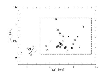
Figure 11.— Spitzer/IRAC colour-colour diagram for the very low mass sources listed in Tables 2 and 4, using the ’HREL’ photometry from the C2D survey. We only plot objects with photometric errors $<40$% in all four bands (41 out of 51). The position of the Class II objects from the survey by Gutermuth et al. (2008) is indicated by the dashed box. Objects with reliable detection at 24$\,\mu m$ are marked with squares

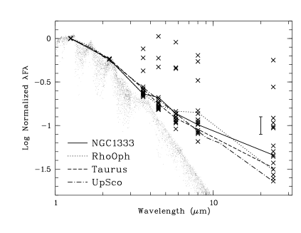
Figure 12.— Spectral energy distributions for 16 very low mass objects with disks in NGC1333 (crosses). The SEDs have been dereddened and scaled to the J-band fluxes. We overplot the typical SED for NGC1333 (solid line), $\rho$ Oph (dotted line) Taurus (dashed line), and UpSco (dash-dotted line). We also show the photospheric SED from the 2800 K DUSTY-AMES model (Allard et al., 2001) with small dots. A typical errorbar for the 24$\,\mu$ fluxes is overplotted.

In Fig. 12 we show their SEDs after dereddening (see Sect. 3.2) and scaling to the J-band flux (crosses). For comparison, the photospheric SED from a model spectrum is overplotted with small dots. To assess the disk evolution in the substellar regime, we derive the typical SED for NGC1333 and three other star forming regions: $\rho$ Oph (1 Myr), Taurus (2 Myr), and UpSco (5 Myr). For this purpose we selected the objects which are detected in all four IRAC bands and at 24$\,\mu m$. For $\rho$ Oph we started with the census in Muzic et al. (subm.) and made use of the C2D data. For Taurus we used published Spitzer data from Guieu et al. (2007) and Scholz et al. (2006). For UpSco the data from Scholz et al. (2007) was used. When comparing the SEDs from different regions, one has to take into account that the depth of the 24$\,\mu m$ observations is not the same; thus the median SED is affected by incompleteness at low flux levels. Instead we plot the SED for the object that has the 10th highest flux level at 24$\,\mu m$ after converting to $\lambda F_{\lambda}$ and scaling to the J-band flux. This represents an estimate for a typical SED unaffected by the depth of the Spitzer observations and the distance to the cluster. Note that all objects used for this exercise are spectroscopically confirmed members of the respective clusters.

For wavelengths $<8\,\mu m$ the four median SEDs are fairly similar. At 8$\,\mu m$ the SEDs in the youngest regions (NGC1333, $\rho$ Oph) are slightly enhanced. The biggest differences are seen at 24$\,\mu m$, particularly when comparing NGC1333 with UpSco. This is mostly due to the fact that NGC1333 harbours a few objects with unusually strong excess emission, which are missing in UpSco (compare with Fig. 1 in Scholz et al., 2007), indicating that the objects in NGC1333 are in an early evolutionary stage compared with the other regions. As demonstrated in Scholz et al. (2009b) a large spread in 24$\,\mu m$ fluxes, as seen in NGC1333, can easily be explained by a range of flaring angles in the disks.

5. Conclusions

As part of our survey program SONYC, we present a census of very low mass objects in the young cluster NGC1333 based on new follow-up spectroscopy from Subaru/FMOS. To derive reliable spectral types from our data, we define a new spectral index based on the slope of the H-band peak. We find 10 new likely brown dwarfs in this cluster, including one with a spectral type $\sim$L3 and two more with spectral type around or later than M9. These objects have estimated masses of 0.006 to 0.02$\,M_{\odot}$, the least massive objects identified thus far in this region. This demonstrates that the mass function in this cluster extends down to the Deuterium burning limit and beyond. By combining the findings from our SONYC survey with results published by other groups, we compile a sample of 51 objects with spectral types of M5 or later in this cluster, more than half of them found by SONYC. About 30-40 of them are likely to be substellar. The star vs. brown dwarf ratio in NGC1333 is significantly lower than in other nearby star forming regions, possibly indicating environmental differences in the formation of brown dwarfs. We show that the spatial distribution of brown dwarfs in NGC1333 closely follows the distribution of the stars in the cluster. The disk fraction in the brown dwarf sample is $<66$%, lower than for the stellar members, but comparable to the brown dwarf disk fraction in 2-3 Myr old regions. The substellar members in NGC1333 show a large fraction of highly flared disks, evidence for the early evolutionary state of the cluster.

Appendix A Spectroscopically excluded objects

In Tables 6 and 7 we provide a full list of objects for which we obtained spectra and which were not classified as young very low mass objects based on the shape of their near-infrared spectrum (see Sect. 3.1). The spectra come from the first campaign with MOIRCS (Scholz et al., 2009a) and from the second run with FMOS (this paper). Most of these objects are likely to be either young stellar objects in NGC1333 or background stars with effective temperatures above $\sim 3500$ K or spectral type earlier than $\sim$M3. In Table 6 we also give the J- and K-band photometry from 2MASS and the identifiers from the photometric surveys by Lada et al. (1996) and Wilking et al. (2004), if available. Objects without listed identifiers are not known to have a counterpart within 1”.

Table 6Objects excluded by spectroscopy in this paper

$\alpha$(J2000)	$\delta$(J2000)	J (mag)	K (mag)	Sel	Spec	Identifier
03 29 18.71	+31 32 26.4	16.722	13.839	IZ	F
03 29 52.35	+31 28 13.7	14.919	13.829	IZ	F
03 29 48.12	+31 28 29.4	15.550	13.663	IZ	F
03 29 37.80	+31 27 48.4	17.274	15.249	IZ	F
03 29 34.76	+31 29 08.1	13.647	11.532	IZ	F	MBO 43
03 29 11.53	+31 30 05.6	16.740	13.786	IZ	F	[LAL96] 241, 242
03 28 55.74	+31 30 58.0	15.175	13.390	IZ	F	[LAL96] 143
03 28 52.66	+31 32 04.3	16.563	14.730	IZ	F
03 28 46.67	+31 31 35.4	15.647	13.933	IZ	F
03 28 37.55	+31 32 54.5	15.107	14.232	IZ	F
03 28 23.84	+31 32 49.3	14.714	13.655	IZ	F
03 28 44.96	+31 31 09.9	17.057	15.211	IZ	F
03 28 46.24	+31 30 12.1	15.089	14.069	IZ	F	[LAL96] 88
03 29 45.53	+31 26 56.5	14.870	14.023	IZ	F
03 30 05.41	+31 25 13.1	14.921	13.680	IZ	F
03 28 49.48	+31 25 06.6	15.957	13.658	IZ	F	MBO 82
03 29 10.46	+31 23 34.8	15.633	12.762	JK	F	[LAL96] 231
03 28 43.17	+31 26 06.1	15.617	13.384	IZ	F	[LAL96] 78
03 28 37.75	+31 26 32.8	16.847	14.340	IZ	F	[LAL96] 60
03 27 56.27	+31 27 00.8	16.836	13.967	IZ	F
03 28 07.64	+31 26 42.4	15.974	13.719	IZ	F
03 28 19.51	+31 26 39.5	15.100	13.687	IZ	F	[LAL96] 13
03 28 40.22	+31 25 49.1	15.637	12.911	IZ	F
03 28 47.64	+31 24 06.2	14.199	11.660	JK	F	[LAL96] 93
03 28 55.22	+31 25 22.4	14.735	12.550	IZ	F	[LAL96] 139
03 29 03.32	+31 23 14.8	17.254	14.071	JK	F	[LAL96] 191
03 29 03.13	+31 22 38.2	13.724	11.323	JK	F	[LAL96] 189
03 29 27.61	+31 21 10.1	14.836	13.074	IZ	F	[LAL96] 324
03 29 55.50	+31 15 30.5	15.120	14.131	IZ	F
03 29 52.65	+31 17 22.9	16.325	14.970	IZ	F
03 29 39.61	+31 17 43.4			JK	F
03 28 35.46	+31 21 29.9	16.052	14.197	IZ	F	[LAL96] 49
03 28 48.45	+31 20 28.4	16.842	14.283	IZ	F	[LAL96] 100
03 29 10.82	+31 16 42.7	15.652	13.039	JK	F	[LAL96] 235
03 29 21.42	+31 15 55.3	15.396	14.004	IZ	F	[LAL96] 305
03 29 45.41	+31 16 23.2	15.118	13.767	IZ	F
03 29 50.23	+31 15 47.9	16.980	15.106	IZ	F
03 30 01.93	+31 10 50.5	14.374	12.921	IZ	F
03 29 54.78	+31 11 41.7	16.679	15.253	IZ	F
03 29 34.57	+31 11 23.8	16.750	14.643	IZ	F	[LAL96] 351
03 29 36.00	+31 12 49.6	15.522	14.615	IZ	F	[LAL96] 353
03 29 26.11	+31 11 36.9	14.781	12.874	IZ	F	[LAL96] 320
03 28 01.19	+31 17 36.5	15.587	14.136	IZ	F
03 27 52.51	+31 19 38.8	14.973	13.662	IZ	F
03 28 22.90	+31 15 21.7	15.032	13.587	IZ	F	[LAL96] 20
03 29 08.71	+31 12 01.9			IZ	F
03 29 12.24	+31 12 20.5	16.588	14.722	IZ	F	[LAL96] 254
03 29 18.45	+31 11 30.5	16.413	15.530	IZ	F
03 29 31.00	+31 11 20.1	17.052	15.265	IZ	F
03 29 28.99	+31 10 00.3	13.365	10.889	IZ	F	[LAL96] 329
03 29 45.40	+31 10 35.6	14.828	13.516	IZ	F
03 29 46.48	+31 08 43.6	15.205	14.096	IZ	F
03 29 49.16	+31 09 03.7	16.143	14.537	IZ	F
03 29 28.95	+31 07 40.9	15.975	15.199	IZ	F	[LAL96] 330
03 29 24.73	+31 07 26.8			IZ	F
03 29 20.11	+31 08 53.7	15.923	14.813	IZ	F
03 29 09.23	+31 08 55.4	16.330	14.912	IZ	F
03 28 57.45	+31 09 46.5	16.623	12.738	IZ	F	[LAL96] 160
03 28 06.32	+31 10 02.0	15.731	14.579	IZ	F
03 28 22.07	+31 10 42.9	13.867	11.859	IZ	F	[LAL96] 18
03 28 39.01	+31 08 07.6	15.143	13.389	IZ	F	[LAL96] 65
03 29 03.60	+31 07 11.9	14.995	13.351	IZ	F	[LAL96] 197
03 29 05.23	+31 07 10.6	16.776	14.766	IZ	F

Table 7Objects excluded by spectroscopy by Scholz et al. (2009a)

$\alpha$(J2000)	$\delta$(J2000)	J (mag)	K (mag)	Sel	Spec	Identifier
03 28 41.72	+31 11 15.1			IZ	M
03 28 41.97	+31 12 17.2	15.863	13.822	IZ	M
03 28 46.21	+31 12 03.4	16.933	13.526	IZ	M	[LAL96] 90
03 28 48.99	+31 12 45.1	17.836	14.048	IZ	M	[LAL96] 103
03 28 52.10	+31 16 29.3	16.071	13.738	IZ	M	[LAL96] 123
03 28 57.25	+31 07 26.0			IZ	M	[LAL96] 159
03 28 58.68	+31 09 39.2	17.052	12.945	IZ	M	[LAL96] 169
03 29 00.70	+31 22 00.8	16.236	11.764	IZ	M	[LAL96] 180
03 29 17.93	+31 14 53.5	16.625	14.039	IZ	M	[LAL96] 287
03 29 18.66	+31 20 17.8	17.510	14.608	IZ	M	MBO 109
03 29 19.86	+31 18 47.7	17.205	13.321	IZ	M	[LAL96] 297
03 29 28.06	+31 18 39.0	15.307	12.846	IZ	M	[LAL96] 327
03 29 32.20	+31 17 07.3	15.503	13.784	IZ	M	[LAL96] 341
03 29 37.41	+31 17 41.6	14.886	12.761	IZ	M	[LAL96] 359
03 29 08.17	+31 11 54.6	17.247	14.980	IZ	M	[LAL96] 217

References

- Allard et al. (2001) Allard, F., Hauschildt, P. H., Alexander, D. R., Tamanai, A., & Schweitzer, A. 2001, ApJ, 556, 357
- Allers et al. (2007) Allers, K. N., Jaffe, D. T., Luhman, K. L., & et al. 2007, ApJ, 657, 511
- Allers et al. (2006) Allers, K. N., Kessler-Silacci, J. E., Cieza, L. A., & Jaffe, D. T. 2006, ApJ, 644, 364
- Andersen et al. (2008) Andersen, M., Meyer, M. R., Greissl, J., & Aversa, A. 2008, ApJ, 683, L183
- Andersen et al. (2011) Andersen, M., Meyer, M. R., Robberto, M., Bergeron, L. E., & Reid, N. 2011, ArXiv e-prints
- Aspin et al. (1994) Aspin, C., Sandell, G., & Russell, A. P. G. 1994, A&AS, 106, 165
- Baraffe et al. (1998) Baraffe, I., Chabrier, G., Allard, F., & Hauschildt, P. H. 1998, A&A, 337, 403
- Baraffe et al. (2002) —. 2002, A&A, 382, 563
- Baraffe et al. (2003) Baraffe, I., Chabrier, G., Barman, T. S., Allard, F., & Hauschildt, P. H. 2003, A&A, 402, 701
- Bate (2009) Bate, M. R. 2009, MNRAS, 392, 590
- Belikov et al. (2002) Belikov, A. N., Kharchenko, N. V., Piskunov, A. E., Schilbach, E., & Scholz, R.-D. 2002, A&A, 387, 117
- Bihain et al. (2010) Bihain, G., Rebolo, R., Zapatero Osorio, M. R., Béjar, V. J. S., & Caballero, J. A. 2010, A&A, 519, A93+
- Bonnell et al. (2008) Bonnell, I. A., Clark, P., & Bate, M. R. 2008, MNRAS, 389, 1556
- Bonnell et al. (2007) Bonnell, I. A., Larson, R. B., & Zinnecker, H. 2007, in Protostars and Planets V, ed. B. Reipurth, D. Jewitt, & K. Keil, 149–164
- Brandeker et al. (2006) Brandeker, A., Jayawardhana, R., Ivanov, V. D., & Kurtev, R. 2006, ApJ, 653, L61
- Briceño et al. (2002) Briceño, C., Luhman, K. L., Hartmann, L., Stauffer, J. R., & Kirkpatrick, J. D. 2002, ApJ, 580, 317
- Burgasser et al. (2008) Burgasser, A. J., Liu, M. C., Ireland, M. J., Cruz, K. L., & Dupuy, T. J. 2008, ApJ, 681, 579
- Burgasser & McElwain (2006) Burgasser, A. J., & McElwain, M. W. 2006, AJ, 131, 1007
- Burgess et al. (2009) Burgess, A. S. M., Moraux, E., Bouvier, J., & et al. 2009, A&A, 508, 823
- Caballero et al. (2008) Caballero, J. A., Burgasser, A. J., & Klement, R. 2008, A&A, 488, 181
- Cameron (2011) Cameron, E. 2011, Publications of the Astronomical Society of Australia, 28, 128
- Cardelli et al. (1989) Cardelli, J. A., Clayton, G. C., & Mathis, J. S. 1989, ApJ, 345, 245
- Cernis (1990) Cernis, K. 1990, Ap&SS, 166, 315
- Chabrier et al. (2000) Chabrier, G., Baraffe, I., Allard, F., & Hauschildt, P. 2000, ApJ, 542, 464
- Cushing et al. (2005) Cushing, M. C., Rayner, J. T., & Vacca, W. D. 2005, ApJ, 623, 1115
- Dawson et al. (2011) Dawson, P., Scholz, A., & Ray, T. P. 2011, ArXiv e-prints
- de Zeeuw et al. (1999) de Zeeuw, P. T., Hoogerwerf, R., de Bruijne, J. H. J., Brown, A. G. A., & Blaauw, A. 1999, AJ, 117, 354
- Evans et al. (2009) Evans, N. J., Dunham, M. M., Jørgensen, J. K., & et al. 2009, ApJS, 181, 321
- Geers et al. (2011) Geers, V., Scholz, A., Jayawardhana, R., & et al. 2011, ApJ, 726, 23
- Greissl et al. (2007) Greissl, J., Meyer, M. R., Wilking, B. A., Fanetti, T., Schneider, G., Greene, T. P., & Young, E. 2007, AJ, 133, 1321
- Guieu et al. (2007) Guieu, S., Pinte, C., Monin, J., Ménard, F., Fukagawa, M., & et al. 2007, A&A, 465, 855
- Gutermuth et al. (2008) Gutermuth, R. A., Myers, P. C., Megeath, S. T., & et al. 2008, ApJ, 674, 336
- Helling et al. (2008) Helling, C., Dehn, M., Woitke, P., & Hauschildt, P. H. 2008, ApJ, 675, L105
- Kimura et al. (2010) Kimura, M., Maihara, T., Iwamuro, F., & et al. 2010, PASJ, 62, 1135
- Kirkpatrick et al. (2006) Kirkpatrick, J. D., Barman, T. S., Burgasser, A. J., & et al. 2006, ApJ, 639, 1120
- Lada et al. (1996) Lada, C. J., Alves, J., & Lada, E. A. 1996, AJ, 111, 1964
- Lafrenière et al. (2011) Lafrenière, D., Jayawardhana, R., Janson, M., & et al. 2011, ApJ, 730, 42
- Lafrenière et al. (2010) Lafrenière, D., Jayawardhana, R., & van Kerkwijk, M. H. 2010, ApJ, 719, 497
- Looper et al. (2007) Looper, D. L., Burgasser, A. J., Kirkpatrick, J. D., & Swift, B. J. 2007, ApJ, 669, L97
- Lucas & Roche (2000) Lucas, P. W., & Roche, P. F. 2000, MNRAS, 314, 858
- Luhman (2007) Luhman, K. L. 2007, ApJS, 173, 104
- Luhman et al. (2008) Luhman, K. L., Hernández, J., Downes, J. J., Hartmann, L., & Briceño, C. 2008, ApJ, 688, 362
- Luhman et al. (2003) Luhman, K. L., Stauffer, J. R., Muench, A. A., & et al. 2003, ApJ, 593, 1093
- Mentuch et al. (2008) Mentuch, E., Brandeker, A., van Kerkwijk, M. H., Jayawardhana, R., & Hauschildt, P. H. 2008, ApJ, 689, 1127
- Mohanty et al. (2007) Mohanty, S., Jayawardhana, R., Huélamo, N., & Mamajek, E. 2007, ApJ, 657, 1064
- Muench et al. (2007) Muench, A. A., Lada, C. J., Luhman, K. L., Muzerolle, J., & Young, E. 2007, AJ, 134, 411
- Muench et al. (2002) Muench, A. A., Lada, E. A., Lada, C. J., & Alves, J. 2002, ApJ, 573, 366
- Mužić et al. (2011) Mužić, K., Scholz, A., Geers, V., Fissel, L., & Jayawardhana, R. 2011, ApJ, 732, 86
- Natta et al. (2004) Natta, A., Testi, L., Muzerolle, J., & et al. 2004, A&A, 424, 603
- Oppenheimer et al. (2000) Oppenheimer, B. R., Kulkarni, S. R., & Stauffer, J. R. 2000, Protostars and Planets IV, 1313
- Padoan et al. (2009) Padoan, P., Juvela, M., Kritsuk, A., & Norman, M. L. 2009, ApJ, 707, L153
- Padoan & Nordlund (2004) Padoan, P., & Nordlund, Å. 2004, ApJ, 617, 559
- Patience et al. (2010) Patience, J., King, R. R., de Rosa, R. J., & Marois, C. 2010, A&A, 517, A76+
- Preibisch et al. (2003) Preibisch, T., Stanke, T., & Zinnecker, H. 2003, A&A, 409, 147
- Quillen et al. (2005) Quillen, A. C., Thorndike, S. L., Cunningham, A., & et al. 2005, ApJ, 632, 941
- Reipurth & Clarke (2001) Reipurth, B., & Clarke, C. 2001, AJ, 122, 432
- Scholz et al. (2009a) Scholz, A., Geers, V., Jayawardhana, R., & et al. 2009a, ApJ, 702, 805
- Scholz et al. (2006) Scholz, A., Jayawardhana, R., & Wood, K. 2006, ApJ, 645, 1498
- Scholz et al. (2007) Scholz, A., Jayawardhana, R., Wood, K., & et al. 2007, ApJ, 660, 1517
- Scholz et al. (2009b) Scholz, A., Xu, X., Jayawardhana, R., & et al. 2009b, MNRAS, 398, 873
- Skemer et al. (2011) Skemer, A. J., Close, L. M., Szücs, L., & et al. 2011, ApJ, 732, 107
- Slesnick et al. (2004) Slesnick, C. L., Hillenbrand, L. A., & Carpenter, J. M. 2004, ApJ, 610, 1045
- Stamatellos & Whitworth (2009) Stamatellos, D., & Whitworth, A. P. 2009, MNRAS, 392, 413
- Umbreit et al. (2005) Umbreit, S., Burkert, A., Henning, T., Mikkola, S., & Spurzem, R. 2005, ApJ, 623, 940
- Weights et al. (2009) Weights, D. J., Lucas, P. W., Roche, P. F., Pinfield, D. J., & Riddick, F. 2009, MNRAS, 392, 817
- Wilking et al. (2004) Wilking, B. A., Meyer, M. R., Greene, T. P., Mikhail, A., & Carlson, G. 2004, AJ, 127, 1131
- Winston et al. (2009) Winston, E., Megeath, S. T., Wolk, S. J., & et al. 2009, AJ, 137, 4777
- Zapatero Osorio et al. (2000) Zapatero Osorio, M. R., Béjar, V. J. S., Martín, E. L., & et al. 2000, Science, 290, 103