Shape constrained nonparametric estimators of the baseline distribution in Cox proportional hazards model

Abstract

We investigate nonparametric estimation of a monotone baseline hazard and a decreasing baseline density within the Cox model. Two estimators of a nondecreasing baseline hazard function are proposed. We derive the nonparametric maximum likelihood estimator and consider a Grenander type estimator, defined as the left-hand slope of the greatest convex minorant of the Breslow estimator. We demonstrate that the two estimators are strongly consistent and asymptotically equivalent and derive their common limit distribution at a fixed point. Both estimators of a nonincreasing baseline hazard and their asymptotic properties are acquired in a similar manner. Furthermore, we introduce a Grenander type estimator for a nonincreasing baseline density, defined as the left-hand slope of the least concave majorant of an estimator of the baseline cumulative distribution function, derived from the Breslow estimator. We show that this estimator is strong consistent and derive its asymptotic distribution at a fixed point.

Keywords: Breslow estimator, Cox model, shape constrained nonparametric maximum likelihood

Running headline: Shape constrained estimation in the Cox model

1 Introduction

Shape constrained nonparametric estimation dates back to the $1950$s. The milestone paper of Grenander [8] introduced the maximum likelihood estimator of a nonincreasing density, while Prakasa Rao [19] derived its asymptotic distribution at a fixed point. Similarly, the maximum likelihood estimator of a monotone hazard function has been proposed by Marshall and Proschan [17] and its asymptotic distribution was determined in [20]. Other estimators have been proposed and despite the high interest and applicability, the difficulty in the derivation of the asymptotics was a major drawback. Shape constrained estimation was revived by Groeneboom [9], who proposed an alternative for Prakasa Rao’s bothersome type of proof. Groeneboom’s approach employs a so-called inverse process and makes use of the Hungarian embedding [15]. Once such an embedding is available, it enables the derivation of the asymptotic distribution of the considered estimator. This is the case, for example, when estimating a monotone density or hazard function from right-censored observations, as proposed by Huang and Zhang [12] and Huang and Wellner [11]. Another setting for deriving the asymptotic distribution, that does not require a Hungarian embedding, was later provided by the limit theorems in [14]. Their cube root asymptotics are based on a functional limit theorem for empirical processes.

The present paper treats the estimation of a monotone baseline hazard and a decreasing baseline density in the Cox model. Ever since the model was introduced (see [4]) and in particular, since the asymptotic properties of the proposed estimators were first derived by Tsiatis [24], the Cox model is the classical survival analysis framework for incorporating covariates in the study of a lifetime distribution. The hazard function is of particular interest in survival analysis, as it represents an important feature of the time course of a process under study, e.g., death or a certain disease. The main reason lies in its ease of interpretation and in the fact that the hazard function takes into account ageing, while, for example, the density function does not. Times to death, infection or development of a disease of interest in most survival analysis studies are observed to have a nondecreasing baseline hazard. Nevertheless, the survival time after a successful medical treatment is usually modeled using a nonincreasing hazard. An example of nonincreasing hazard is presented in Cook et al. [3], where the authors concluded that the daily risk of pneumonia decreases with increasing duration of stay in the intensive care unit.

Chung and Chang [2] consider a maximum likelihood estimator of a nondecreasing baseline hazard function in the Cox model, adopting the convention that each censoring time is equal to its preceding observed event time. They prove consistency, but no distributional theory is available. We consider a maximum likelihood estimator $\hat{\lambda}_{n}$ of a monotone baseline hazard function, which imposes no extra assumption on the censoring times. This estimator differs from the one in [2] and has a higher likelihood. Furthermore, we introduce a Grenander type estimator for a monotone baseline hazard function based on the well-known baseline cumulative hazard estimator, the Breslow estimator $\Lambda_{n}$ [4]. The nondecreasing baseline hazard estimator $\tilde{\lambda}_{n}$ is defined as the left-hand slope of the greatest convex minorant (GCM) of $\Lambda_{n}$. Similarly, a nonincreasing baseline estimator is characterized as the left-hand slope of the least concave majorant (LCM) of $\Lambda_{n}$. It is noteworthy that, just as in the no covariates case (see [11]), the two monotone estimators are different, but are shown to be asymptotically equivalent. Additionally, we introduce a nonparametric estimator for a nonincreasing baseline density. An estimator $F_{n}$ for the baseline distribution function is based on the Breslow estimator and next, the baseline density estimator $\tilde{f}_{n}$ is defined as the left-hand slope of the LCM of $F_{n}$. The treatment of the maximum likelihood estimator for a nonincreasing baseline density is much more complex and is deferred to another paper. For the remaining three estimators, we show that they converge at rate $n^{1/3}$ and we establish their limit distribution. Since, to the authors best knowledge, there does not exist a Hungarian embedding for the Breslow estimator, our results are based on the theory in [14] and an argmax continuous mapping theorem in [11].

The paper is organized as follows. In Section 2 we introduce the model and state our assumptions. The formal characterization of the maximum likelihood estimator $\hat{\lambda}_{n}$ is given in Lemmas 1 and 2. Our main results concerning the asymptotic properties of the proposed estimators are gathered in Section 3. Section 4 is devoted to proving the strong consistency results of the paper. The strong uniform consistency of the Breslow estimator in Theorem 5 and of the baseline cumulative distribution estimator $F_{n}$ in Corollary 1, emerge as necessary results. These results are preceded by three preparatory lemmas, that establish properties of functionals in terms of which derivations thereof can be expressed. In order to prepare the application of results from [14], in Section 5 we introduce the inverses of the estimators in terms of minima and maxima of random processes and obtain the limiting distribution of these processes. Finally, in Section 6, we derive the asymptotic distribution of the estimators, at a fixed point. The proofs of some preparatory lemmas are deferred to an appendix, which is available in the online Supporting Information.

2 Definitions and assumptions

Let the observed data consist of independent identically distributed triplets $\left(T_{i},\Delta_{i},Z_{i}\right)$, with $i=1,2,\ldots,n$, where $T_{i}$ denotes the follow-up time, with a corresponding censoring indicator $\Delta_{i}$ and covariate vector $Z_{i}\in\mathbbm{R}^{p}$. A generic follow-up time is defined by $T=\text{min}\left(X,C\right)$, where $X$ represents the event time and $C$ is the censoring time. Accordingly, $\Delta=\left\{X\leq C\right\}$, where $\{\cdot\}$ denotes the indicator function. The event time $X$ and censoring time $C$ are assumed to be conditionally independent given $Z$, and the censoring mechanism is assumed to be non-informative. The covariate vector $Z\in\mathbb{R}^{p}$ is assumed to be time invariant.

Within the Cox model, the distribution of the event time is related to the corresponding covariate by

$$\lambda\left(x|z\right)=\lambda_{0}(x)\,\text{e}^{\beta_{0}^{\prime}z},$$ (1)

where $\lambda\left(x|z\right)$ is the hazard function for an individual with covariate vector $z\in\mathbb{R}^{p}$, $\lambda_{0}$ represents the baseline hazard function and $\beta_{0}\in\mathbbm{R}^{p}$ is the vector of the underlying regression coefficients. Conditionally on $Z=z$, the event time $X$ is assumed to be a nonnegative random variable with an absolutely continuous distribution function $F(x|z)$ with density $f(x|z)$. The same assumptions hold for the censoring variable $C$ and its distribution function $G$. The distribution function of the follow-up time $T$ is denoted by $H$. We will assume the following conditions, which are commonly employed in deriving large sample properties of Cox proportional hazards estimators (e.g., see [24]).

(A1) Let $\tau_{F},\tau_{G}$ and $\tau_{H}$ be the end points of the support of $F,G$ and $H$ respectively. Then

$$\tau_{H}=\tau_{G}<\tau_{F}\leq\infty.$$

(A2) There exists $\varepsilon>0$ such that

$$\sup_{|\beta-\beta_{0}|\leq\varepsilon}\mathbbm{E}\left[|Z|^{2}\,\text{e}^{2\beta^{\prime}Z}\right]<\infty,$$

where $|\cdot|$ denotes the Euclidean norm.

2.1 Increasing baseline hazard

Let $\Lambda(x|z)=-\log(1-F(x|z))$ be the cumulative hazard function. Then, from (1) it follows that $\Lambda(x|z)=\Lambda_{0}(x)\exp(\beta_{0}^{\prime}z)$, where $\Lambda_{0}(x)=\int_{0}^{x}\lambda_{0}(u)\,\mathrm{d}u$ denotes the baseline cumulative hazard function. When $G$ has a density $g$, then together with the relation $\lambda=f/(1-F)$, the likelihood becomes

$$\begin{split}&\prod_{i=1}^{n}\Big{[}f(T_{i}\mid Z_{i})(1-G(T_{i}\mid Z_{i}))\Big{]}^{\Delta_{i}}\Big{[}g(T_{i}\mid Z_{i})(1-F(T_{i}\mid Z_{i}))\Big{]}^{1-\Delta_{i}}\\ &=\prod_{i=1}^{n}\lambda(T_{i}\mid Z_{i})^{\Delta_{i}}\exp\Big{(}-\Lambda(T_{i}\mid Z_{i})\Big{)}\times\prod_{i=1}^{n}\Big{[}1-G(T_{i}\mid Z_{i})\Big{]}^{\Delta_{i}}g(T_{i}\mid Z_{i})^{1-\Delta_{i}}.\end{split}$$

The term with $g$ does not involve the baseline distribution and can be treated as a constant term. Therefore, one essentially needs to maximize

$$\prod_{i=1}^{n}\lambda(T_{i}\mid Z_{i})^{\Delta_{i}}\exp\Big{(}-\Lambda(T_{i}\mid Z_{i})\Big{)}=\prod_{i=1}^{n}\Big{[}\lambda_{0}(T_{i})\mathrm{e}^{\beta_{0}^{\prime}Z_{i}}\Big{]}^{\Delta_{i}}\exp\Big{(}-\mathrm{e}^{\beta_{0}^{\prime}Z_{i}}\Lambda_{0}(T_{i})\Big{)}.$$

This leads to the following (pseudo) loglikelihood, written as a function of $\beta\in\mathbb{R}^{p}$ and $\lambda_{0}$,

$$\sum_{i=1}^{n}\left[\Delta_{i}\log\lambda_{0}(T_{i})+\Delta_{i}\beta^{\prime}Z_{i}-\text{e}^{\beta^{\prime}Z_{i}}\Lambda_{0}(T_{i})\right].$$ (2)

Remark 1.

It may be worthwhile to note that if the censoring distribution is discrete, the likelihood of $(T,\Delta,Z)$ can still be written as

$$[f(T\mid Z)(1-G(T\mid Z))]^{\Delta}[g(T\mid Z)(1-F(T\mid Z))]^{1-\Delta},$$

where $g(y|z)=P(C=y|Z=z)$, which will lead to the same expression as in (2). However, as we will make use of other results in the literature that are established under the assumption of an absolutely continuous censoring distribution (e.g., from [24]), we do not further investigate the behavior of our estimators in the case of a discrete censoring distribution.

For $\beta\in\mathbb{R}^{p}$ fixed, we first consider maximum likelihood estimation for a nondecreasing $\lambda_{0}$. This requires the maximization of (2) over all nondecreasing $\lambda_{0}$. Let $T_{(1)}<T_{(2)}<\cdots<T_{(n)}$ be the ordered follow-up times and, for $i=1,2,\ldots,n$, let $\Delta_{(i)}$ and $Z_{(i)}$ be the censoring indicator and covariate vector corresponding to $T_{(i)}$. The characterization of the maximizer $\hat{\lambda}_{n}(x;\beta)$ can be described by means of the processes

$$W_{n}(\beta,x)=\int\left(\text{e}^{\beta^{\prime}z}\int_{0}^{x}\{u\geq s\}\,\mathrm{d}s\right)\,\mathrm{d}\mathbbm{P}_{n}(u,\delta,z),$$ (3)

and

$$V_{n}(x)=\int\delta\{u<x\}\,\mathrm{d}\mathbbm{P}_{n}(u,\delta,z),$$ (4)

with $\beta\in\mathbb{R}^{p}$ and $x\geq 0$, where $\mathbbm{P}_{n}$ is the empirical measure of the $(T_{i},\Delta_{i},Z_{i})$ and is given by the following lemma.

Lemma 1.

For a fixed $\beta\in\mathbbm{R}^{p}$, let $W_{n}$ and $V_{n}$ be defined in (3) and (4). Then, the NPMLE $\hat{\lambda}_{n}(x;\beta)$ of a nondecreasing baseline hazard function $\lambda_{0}$ is of the form

$$\hat{\lambda}_{n}(x;\beta)=\begin{cases}0&x<T_{(1)},\\ \hat{\lambda}_{i}&T_{(i)}\leq x<T_{(i+1)},\text{ for }i=1,2,\ldots,n-1,\\ \infty&x\geq T_{(n)},\end{cases}$$

where $\hat{\lambda}_{i}$ is the left derivative of the greatest convex minorant at the point $P_{i}$ of the cumulative sum diagram consisting of the points

$$P_{j}=\Big{(}W_{n}(\beta,T_{(j+1)})-W_{n}(\beta,T_{(1)}),V_{n}(T_{(j+1)})\Big{)},$$

for $j=1,2,\ldots,n-1$ and $P_{0}=(0,0)$. Furthermore,

$$\hat{\lambda}_{i}=\max_{1\leq s\leq i}\,\,\min_{i\leq t\leq n-1}\frac{\sum_{j=s}^{t}\Delta_{(j)}}{\sum_{j=s}^{t}\left(T_{(j+1)}-T_{(j)}\right)\sum_{l=j+1}^{n}\text{e}^{\beta^{\prime}Z_{(l)}}},$$ (5)

for $i=1,2,\ldots,n-1$.

Proof.

Similar to [17] and Section 7.4 in [22], since $\lambda_{0}(T_{(n)})$ can be chosen arbitrarily large, we first consider the maximization over nondecreasing $\lambda_{0}$ bounded by some $M>0$. When we increase the value of $\lambda_{0}$ on an interval $(T_{(i-1)},T_{(i)})$, the terms $\lambda_{0}(T_{(i)})$ in (2) are not changed, whereas terms with $\Lambda_{0}(T_{(i)})$ will decrease the loglikelihood. Since $\lambda_{0}$ must be nondecreasing, we conclude that the solution is a nondecreasing step function, that is zero for $x<T_{(1)}$, constant on $[T_{(i)},T_{(i+1)})$, for $i=1,2,\ldots,n-1$, and equal to $M$, for $x\geq T_{(n)}$. Consequently, for $\beta\in\mathbb{R}^{p}$ fixed, the (pseudo) loglikelihood reduces to

$$\begin{split}L_{\beta}(\lambda_{0})&=\sum_{i=1}^{n-1}\Delta_{(i)}\log\lambda_{0}(T_{(i)})-\sum_{i=2}^{n}\text{e}^{\beta^{\prime}Z_{(i)}}\sum_{j=1}^{i-1}\left(T_{(j+1)}-T_{(j)}\right)\lambda_{0}(T_{(j)})\\ &=\sum_{i=1}^{n-1}\left[\Delta_{(i)}\log\lambda_{0}(T_{(i)})-\lambda_{0}(T_{(i)})\left(T_{(i+1)}-T_{(i)}\right)\sum_{l=i+1}^{n}\text{e}^{\beta^{\prime}Z_{(l)}}\right].\end{split}$$ (6)

Maximization over $0\leq\lambda_{0}(T_{(1)})\leq\cdots\leq\lambda_{0}(T_{(n-1)})\leq M$ will then have a solution $\hat{\lambda}_{n}^{M}(x;\beta)$ and by letting $M\to\infty$, we obtain the NPMLE $\hat{\lambda}_{n}(x;\beta)$ for $\lambda_{0}$.

First, notice that the loglikelihood function in (6) can also be written as

$$\begin{split}\sum_{i=1}^{n-1}\Big{[}s_{i}\log\lambda_{0}(T_{(i)})-\lambda_{0}(T_{(i)})\Big{]}w_{i},\end{split}$$ (7)

where, for $i=1,2,\ldots,n-1$,

$$w_{i}=\left(T_{(i+1)}-T_{(i)}\right)\sum_{l=i+1}^{n}\text{e}^{\beta^{\prime}Z_{(l)}},$$

and

$$s_{i}=\frac{\Delta_{(i)}}{\left(T_{(i+1)}-T_{(i)}\right)\sum_{l=i+1}^{n}\text{e}^{\beta^{\prime}Z_{(l)}}}.$$

As mentioned above, we first maximize over nondecreasing $\lambda_{0}$ bounded by some $M$. Since $M$ can be chosen arbitrarily large, the problem of maximizing (7) over $0\leq\lambda_{0}(T_{(1)})\leq\cdots\leq\lambda_{0}(T_{(n-1)})\leq M$ can be identified with the problem solved in Example 1.5.7 in [22]. The existence of $\hat{\lambda}_{n}^{M}$ is therefore immediate and is given by

$$\hat{\lambda}_{n}^{M}(x;\beta)=\begin{cases}0&x<T_{(1)},\\ \hat{\lambda}_{i}&T_{(i)}\leq x<T_{(i+1)},\text{ for }i=1,2,\ldots,n-1,\\ M&x\geq T_{(n)},\end{cases}$$

where, as a result of Theorems 1.5.1 and 1.2.1 in [22], the value $\hat{\lambda}_{i}$ is the left derivative at $P_{i}$ of the GCM of the cumulative sum diagram (CSD) consisting of the points

$$P_{i}=\left(\frac{1}{n}\sum_{j=1}^{i}w_{j},\frac{1}{n}\sum_{j=1}^{i}w_{j}s_{j}\right),\qquad i=1,2,\ldots,n-1,$$

and $P_{0}=(0,0)$. It follows that

$$\begin{split}\frac{1}{n}\sum_{j=1}^{i}w_{j}&=\sum_{j=1}^{i}\left(T_{(j+1)}-T_{(j)}\right)\frac{1}{n}\sum_{l=1}^{n}\{T_{l}\geq T_{(j+1)}\}\text{e}^{\beta^{\prime}Z_{l}}\\ &=\int_{T_{(1)}}^{T_{(i+1)}}\int\{u\geq s\}\text{e}^{\beta^{\prime}z}\,\mathrm{d}\mathbbm{P}_{n}(u,\delta,z)\,\mathrm{d}s=W_{n}(\beta,T_{(i+1)})-W_{n}(\beta,T_{(1)}).\end{split}$$

For the $y$-coordinate of the CSD, notice that

$$\frac{1}{n}\sum_{j=1}^{i}w_{j}s_{j}=\frac{1}{n}\sum_{j=1}^{i}\Delta_{(j)}=\frac{1}{n}\sum_{j=1}^{n}\{T_{j}\leq T_{(i)},\Delta_{j}=1\}=V_{n}(T_{(i+1)}).$$

By letting $M\to\infty$, we obtain the NPMLE $\hat{\lambda}_{n}(\beta,x)$ for $\lambda_{0}$. The max-min formula in (5) follows from Theorem 1.4.4 in [22]. ∎

Remark: From the characterization given in Lemma 1, it can be seen that the GCM of the CSD only changes slope at points corresponding to uncensored observations, which means that $\hat{\lambda}_{n}(x;\beta)$ is constant between successive uncensored follow-up times. Moreover, similar to the reasoning in the proof of Lemma 1, it follows that $\hat{\lambda}_{n}(x;\beta)$ maximizes (2). The reason to provide the characterization in Lemma 1 in terms of all follow-up times is that this facilitates the treatment of the asymptotics for this estimator. Finally, for the solution $\hat{\lambda}_{n}^{M}(x;\beta)$, on the interval $[T_{(n)},\tau_{H})$, in principle one could take any value between $\hat{\lambda}_{n-1}$ and $M$. This means that for $\hat{\lambda}_{n}(x;\beta)$, on the interval $[T_{(n)},\tau_{H})$, one could take any value larger than $\hat{\lambda}_{n-1}$.

In practice, one also has to estimate $\beta_{0}$. The standard choice is $\hat{\beta}_{n}$, the maximizer of the partial likelihood function

$$\prod_{l=1}^{m}\frac{\text{e}^{\beta^{\prime}Z_{j}}}{\sum_{j=1}^{n}\{T_{j}\geq X_{(i)}\}\text{e}^{\beta^{\prime}Z_{j}}},$$

as proposed by Cox [4, 5], where $X_{(1)}<X_{(2)}<\cdots<X_{(m)}$ denote the ordered, observed event times. Since the maximum partial likelihood estimator $\hat{\beta}_{n}$ for $\beta_{0}$ is asymptotically efficient under mild conditions and because the amount of information on $\beta_{0}$ lost through lack of knowledge of $\lambda_{0}$ is usually small (see e.g.,[7, 18, 23]), we do not pursue joint maximization of (2) over nondecreasing $\lambda_{0}$ and $\beta_{0}$. We simply replace $\beta$ in $\hat{\lambda}_{n}(x;\beta)$ by $\hat{\beta}_{n}$, and we propose $\hat{\lambda}_{n}(x)=\hat{\lambda}_{n}(x;\hat{\beta}_{n})$ as our estimator for $\lambda_{0}$.

Note that $\hat{\lambda}_{n}$ is different from the estimator derived in [2], where each censoring time is taken equal to the preceding observed event time. This leads to a CSD that is slightly different from the one in Lemma 1. However, it can be shown that both estimators have the same asymptotic behavior. Furthermore, if we take all covariates equal to zero, the model coincides with the ordinary random censorship model with a nondecreasing hazard function as considered in [11]. The characterization in Lemma 1, with all $Z_{l}\equiv 0$, differs slightly from the one in Theorem 3.2 in [11]. Their estimator seems to be the result of maximization of (2) over left-continuous $\lambda_{0}$ that are constant between follow-up times. Although this estimator does not maximize (2) over all nondecreasing $\lambda_{0}$, the asymptotic distribution will turn out to be the same as that of $\hat{\lambda}_{n}$, for the special case of no covariates. The computation of joint maximum likelihood estimates for $\beta$ and $\lambda_{0}$ is considered in [13], who also developed an R package to compute the estimates.

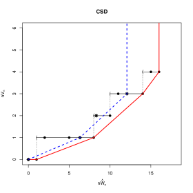
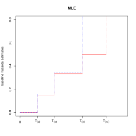
Figure 1: The cumulative sum diagrams along with their GCM (left panel) and the corresponding estimates of a nondecreasing baseline hazard (right panel). Black points and solid curves correspond to the estimator in Lemma 1; star points and dashed curves correspond to the estimator in [2].

To illustrate the computation of the estimator described in Lemma 1, consider an artificial survival dataset consisting of $10$ follow-up times, with only $T_{(2)},T_{(5)},T_{(6)}$, and $T_{(8)}$ being observed event times. In Figure 1 we illustrate the construction of the proposed estimator and compare the resulting estimate with the one suggested in [2]. In order to compare the CSD of both estimates, the coordinates of the CSD described in Lemma 1 have been multiplied with a factor $n$, which obviously leads to the same slopes. Figure 1 displays the points of the CSD (black points) and the GCM (solid curve) in the left panel. The horizontal segments are generated by $(nW_{n}(\hat{\beta}_{n},x)-nW_{n}(\hat{\beta}_{n},T_{(1)}),nV_{n}(x))$ for $x\geq T_{(1)}$. Note that the process $nV_{n}$ has a jump of size 1 right after a point $P_{j}$ that corresponds to an observed event time. Taking left derivatives then yield jumps of $\hat{\lambda}_{n}$ only at observed event times. The right panel of Figure 1 displays the corresponding graph of $\hat{\lambda}_{n}$ (solid curve). The jumps of $\hat{\lambda}_{n}$ in the right panel correspond to the changes of slope of the GCM at the points $P_{1},P_{4}$ and $P_{7}$ in the left panel and occur at the event times $T_{(2)},T_{(5)}$, and $T_{(8)}$. The height of the horizontal segments in the right panel corresponds to the slopes of the GCM in the left panel. For comparison we have added the CSD (star points) and the corresponding GCM (dashed curve) of the estimator derived in [2] in the left panel and the resulting estimator in the right panel (dashed curve). Note that shifting the censoring times back to the nearest previous event time, as suggested in [2], pushes points in the CSD, that correspond to event times, to the left. As a consequence this yields steeper slopes in the left panel and hence a larger estimate of the hazard in the right panel.

Figure 1 about here.

Another possibility to estimate a nondecreasing hazard is to construct a Grenander type estimator, i.e., consider an unconstrained estimator $\Lambda_{n}$ for the cumulative hazard $\Lambda_{0}$ and take the left derivative of the GCM as an estimator of $\lambda_{0}$. Several isotonic estimators are of this form (see e.g., [8, 1, 11, 6]). Breslow [4] proposed

$$\Lambda_{n}(x)=\sum_{i|X_{(i)}\leq x}\dfrac{d_{i}}{\sum_{j=1}^{n}\{T_{j}\geq X_{(i)}\}\text{e}^{\hat{\beta}_{n}^{\prime}Z_{j}}},$$ (8)

as an estimator for $\Lambda_{0}$, where $d_{i}$ is the number of events at $X_{(i)}$ and $\hat{\beta}_{n}$ is the maximum partial likelihood estimator of the regression coefficients. The estimator $\Lambda_{n}$ is most commonly referred to as the Breslow estimator. In the case of no covariates, i.e., $\beta=0$, the NPMLE estimate of an increasing hazard rate has been illustrated in [11].

Following the derivations in [24], it can be inferred that

$$\lambda_{0}(x)=\frac{\mathrm{d}H^{uc}(x)/\mathrm{d}x}{\mathbb{E}\left[\{T\geq x\}\exp(\beta_{0}^{\prime}Z)\right]},$$ (9)

where $H^{uc}(x)=\mathbbm{P}(T\leq x,\Delta=1)$ is the sub-distribution function of the uncensored observations. Consequently, it can be derived that

$$\Lambda_{0}(x)=\int\frac{\delta\{u\leq x\}}{\mathbb{E}\left[\{T\geq x\}\exp(\beta_{0}^{\prime}Z)\right]}\,\mathrm{d}P(u,\delta,z),$$ (10)

where $P$ is the underlying probability measure corresponding to the distribution of $(T,\Delta,Z)$. From (A1), it follows that $\Lambda_{0}(\tau_{H})<\infty$. In view of the above expression, an intuitive baseline cumulative hazard estimator is obtained by replacing the expectations in (10) by averages and by plugging in $\hat{\beta}_{n}$, which yields exactly the Breslow estimator in (8). As a Grenander type estimator for a nondecreasing hazard, we propose the left derivative $\tilde{\lambda}_{n}$ of the greatest convex minorant $\widetilde{\Lambda}_{n}$ of $\Lambda_{n}$. This estimator is different from $\hat{\lambda}_{n}$ for finite samples, but we will show that both estimators are asymptotically equivalent. For the special case of no covariates, this coincides with the results in [11].

2.2 Decreasing baseline hazard

A completely similar characterization is provided for the NPMLE of a nonincreasing baseline hazard function. As in the nondecreasing case, one can argue that the loglikelihood is maximized by a decreasing step function that is constant on $(T_{(i-1)},T_{(i)}]$, for $i=1,2,\ldots,n$, where $T_{(0)}=0$. In this case, the loglikelihood reduces to

$$L_{\beta}(\lambda_{0})=\sum_{i=1}^{n}\left[\Delta_{(i)}\log\lambda_{0}(T_{(i)})-\lambda_{0}(T_{(i)})\left(T_{(i)}-T_{(i-1)}\right)\sum_{l=i}^{n}\text{e}^{\beta^{\prime}Z_{(l)}}\right],$$

which is maximized over all $\lambda_{0}(T_{(1)})\geq\cdots\geq\lambda_{0}(T_{(n)})\geq 0$. The solution is characterized by the following lemma. The proof of this lemma is completely similar to that of Lemma 1.

Lemma 2.

For a fixed $\beta\in\mathbbm{R}^{p}$, let $W_{n}$ be defined in (3) and let

$$Y_{n}(x)=\int\delta\{u\leq x\}\,\mathrm{d}\mathbb{P}_{n}(u,\delta,z).$$ (11)

Then the NPMLE $\hat{\lambda}_{n}(x;\beta)$ of a nonincreasing baseline hazard function $\lambda_{0}$ is given by

$$\hat{\lambda}_{n}(x;\beta)=\hat{\lambda}_{i}\qquad\text{for }x\in(T_{(i-1)},T_{(i)}],$$

for $i=1,2,\ldots,n$, where $\hat{\lambda}_{i}$ is the left derivative of the least concave majorant (LCM) at the point $P_{i}$ of the cumulative sum diagram consisting of the points

$$P_{j}=\Big{(}W_{n}(\beta,T_{(j)}),Y_{n}(T_{(j)})\Big{)},$$

for $j=1,2,\ldots,n$ and $P_{0}=(0,0)$. Furthermore,

$$\hat{\lambda}_{i}=\max_{1\leq s\leq i}\,\,\min_{i\leq t\leq n}\frac{\sum_{j=s}^{t}\Delta_{(j)}}{\sum_{j=s}^{t}\left(T_{(j)}-T_{(j-1)}\right)\sum_{l=j}^{n}\text{e}^{\beta^{\prime}Z_{(l)}}},$$

for $i=1,2,\ldots,n$.

Analogous to the nondecreasing case, for $x\geq T_{(n)}$, one can choose for $\hat{\lambda}_{n}(x;\beta)$ any value smaller than $\hat{\lambda}_{n}$. As before, we propose $\hat{\lambda}_{n}(x)=\hat{\lambda}_{n}(x;\hat{\beta}_{n})$ as an estimator for $\lambda_{0}$, where $\hat{\beta}_{n}$ denotes the maximum partial likelihood estimator for $\beta_{0}$. Similar to the nondecreasing case, the Grenander type estimator $\tilde{\lambda}_{n}$ for a nonincreasing $\lambda_{0}$ is defined as the left-hand slope of the LCM of the Breslow estimator $\Lambda_{n}$, defined in (8).

An illustration of the NPMLE of a decreasing baseline hazard function can be found in [26], who investigated the hazard of patients with acute coronary syndrome. Previous clinical trials indicated a decreasing risk pattern, which the authors confirmed by a test based on a bootstrap procedure. The above estimate has been computed for 1200 patients undergoing early or selective invasive strategies, that were monitored for five years, and their performance was evaluated by means of a simulation experiment. The R code is available in the online version of their paper.

2.3 Decreasing baseline density

Suppose one is interested in estimating a nonincreasing baseline density $f_{0}(\cdot)=f(\cdot|z=0)$. One might argue that this problem is of less interest, because the monotonicity assumption assumed for $z=0$ may no longer hold if one transforms the covariates by $a+bz$, whereas the Cox model essentially remains unchanged. Whereas the estimator for the baseline hazard remains monotone under such transformations, this may no longer hold for the estimator of the baseline density. Despite this drawback, we feel that the estimation of a nonincreasing baseline density may be of interest.

In this case, the corresponding baseline distribution function $F_{0}$ is concave and it relates to the baseline cumulative hazard function $\Lambda_{0}$ as follows

$$F_{0}(x)=1-\text{e}^{-\Lambda_{0}(x)}.$$ (12)

Hence, a natural estimator of the baseline distribution function is

$$F_{n}(x)=1-\text{e}^{-\Lambda_{n}(x)},$$ (13)

where $\Lambda_{n}$ is the Breslow estimator, defined in (8). A Grenander type estimator $\tilde{f}_{n}$ of a nonincreasing baseline density is defined as the left-hand slope of the LCM of $F_{n}$. Recall that $\Lambda_{n}$ depends on $\hat{\beta}_{n}$ and $Z_{1},Z_{2},\ldots,Z_{n}$, and therefore the same holds for $F_{n}$ and $\tilde{f}_{n}$.

The derivation of the NPMLE for $f_{0}$ is much more complex than the previous estimators and its treatment is postponed to a future manuscript. In the special case of no covariates, the NPMLE $\hat{f}_{n}$ has first been derived in [12]. In [11] a different characterization has been provided for $\hat{f}_{n}$ in terms of a self-induced cusum diagram and it was shown that $\hat{f}_{n}$ and $\tilde{f}_{n}$ are asymptotically equivalent.

3 Main results

In this section, we state our main results. The proofs are postponed to subsequent sections. The next theorem provides pointwise consistency of the proposed estimators at a fixed point $x_{0}$ in the interior of the support. Note that the results below imply that if $x_{0}$ is a point of continuity of $\lambda_{0}$, then $\hat{\lambda}_{n}(x_{0})\to\lambda_{0}(x_{0})$ with probability one, and likewise for the other estimators.

Theorem 1.

Assume that (A1) and (A2) hold.

1. Suppose that $\lambda_{0}$ is nondecreasing on $[0,\infty)$ and let $\hat{\lambda}_{n}$ and $\tilde{\lambda}_{n}$ be the estimators defined in Section 2.1. Then, for any $x_{0}\in(0,\tau_{H})$,

   $$\begin{split}\lambda_{0}(x_{0}-)\leq\liminf_{n\rightarrow\infty}\ \hat{\lambda}_{n}(x_{0})\leq\limsup_{n\rightarrow\infty}\hat{\lambda}_{n}(x_{0})\leq\lambda_{0}(x_{0}+),\\ \lambda_{0}(x_{0}-)\leq\liminf_{n\rightarrow\infty}\ \tilde{\lambda}_{n}(x_{0})\leq\limsup_{n\rightarrow\infty}\tilde{\lambda}_{n}(x_{0})\leq\lambda_{0}(x_{0}+),\end{split}$$

   with probability one, where the values $\lambda_{0}(x_{0}-)$ and $\lambda_{0}(x_{0}+)$ denote the left and right limit at $x_{0}$.

2. Suppose that $\lambda_{0}$ is nonincreasing on $[0,\infty)$ and let $\hat{\lambda}_{n}$ and $\tilde{\lambda}_{n}$ be the estimators defined in Section 2.2. Then, for any $x_{0}\in(0,\tau_{H})$,

   $$\begin{split}\lambda_{0}(x_{0}+)\leq\liminf_{n\rightarrow\infty}\hat{\lambda}_{n}(x_{0})&\leq\limsup_{n\rightarrow\infty}\hat{\lambda}_{n}(x_{0})\leq\lambda_{0}(x_{0}-),\\ \lambda_{0}(x_{0}+)\leq\liminf_{n\rightarrow\infty}\tilde{\lambda}_{n}(x_{0})&\leq\limsup_{n\rightarrow\infty}\tilde{\lambda}_{n}(x_{0})\leq\lambda_{0}(x_{0}-),\end{split}$$

   with probability one.

3. Suppose that $f_{0}$ is nonincreasing on $[0,\infty)$ and let $\tilde{f}_{n}$ be the estimator defined in Section 2.3. Then, for any $x_{0}\in(0,\tau_{H})$,

   $$f_{0}(x_{0}+)\leq\liminf_{n\rightarrow\infty}\tilde{f}_{n}(x_{0})\leq\limsup_{n\rightarrow\infty}\tilde{f}_{n}(x_{0})\leq f_{0}(x_{0}-),$$

   with probability one, where $f_{0}(x_{0}-)$ and $f_{0}(x_{0}+)$ denote the left and right limit at $x_{0}$.

The following two theorems yield the asymptotic distribution of the monotone constrained baseline hazard estimators. In order to keep notations compact, it becomes useful to introduce

$$\Phi(\beta,x)=\int\{u\geq x\}\,\text{e}^{\beta^{\prime}z}\,\mathrm{d}P(u,\delta,z),$$ (14)

for $\beta\in\mathbb{R}^{p}$ and $x\in\mathbb{R}$, where $P$ is the underlying probability measure corresponding to the distribution of $(T,\Delta,Z)$. Furthermore, by the argmin function we mean the supremum of times at which the minimum is attained. Note that the limiting distribution and the rate of convergence coincide with the results commonly obtained for isotonic estimators and differ from the corresponding quantities in the traditional central limit theorem. The limiting distribution, usually referred to as the Chernoff distribution, has been tabulated in [10].

Theorem 2.

Assume (A1) and (A2) and let $x_{0}\in(0,\tau_{H})$. Suppose that $\lambda_{0}$ is nondecreasing on $[0,\infty)$ and continuously differentiable in a neighborhood of $x_{0}$, with $\lambda_{0}(x_{0})\neq 0$ and $\lambda_{0}^{\prime}(x_{0})>0$. Moreover, suppose that $H^{uc}(x)$ and $x\mapsto\Phi(\beta_{0},x)$ are continuously differentiable in a neighborhood of $x_{0}$, where $H^{uc}$ is defined below (9) and $\Phi$ is defined in (14). Let $\hat{\lambda}_{n}$ and $\tilde{\lambda}_{n}$ be the estimators defined in Section 2.1. Then,

$$n^{1/3}\left(\frac{\Phi(\beta_{0},x_{0})}{4\lambda_{0}(x_{0})\lambda_{0}^{\prime}(x_{0})}\right)^{1/3}\left(\hat{\lambda}_{n}(x_{0})-\lambda_{0}(x_{0})\right)\xrightarrow{d}\underset{t\in\mathbbm{R}}{\operatorname{argmin}}\{\mathbbm{W}(t)+t^{2}\},$$ (15)

where $\mathbbm{W}$ is standard two-sided Brownian motion originating from zero. Furthermore,

$$n^{1/3}\left(\tilde{\lambda}_{n}(x_{0})-\hat{\lambda}_{n}(x_{0})\right)\xrightarrow{p}0,$$ (16)

so that the convergence in (15) also holds with $\hat{\lambda}_{n}$ replaced by $\tilde{\lambda}_{n}$.

Let $\overline{\lambda}_{n}$ be the estimator considered in [2], which has been proven to be consistent. Completely similar to the proof of Theorem 2 it can be shown that

$$n^{1/3}\left(\overline{\lambda}_{n}(x_{0})-\hat{\lambda}_{n}(x_{0})\right)\xrightarrow{p}0,$$

so that the convergence in (15) also holds with $\hat{\lambda}_{n}$ replaced by $\overline{\lambda}_{n}$. The next theorem establishes the same results as in Theorem 2, for the nonincreasing case.

Theorem 3.

Assume (A1) and (A2) and let $x_{0}\in(0,\tau_{H})$. Suppose that $\lambda_{0}$ is nonincreasing on $[0,\infty)$ and continuously differentiable in a neighborhood of $x_{0}$, with $\lambda_{0}(x_{0})\neq 0$ and $\lambda_{0}^{\prime}(x_{0})<0$. Moreover, suppose that $H^{uc}(x)$ and $x\mapsto\Phi(\beta_{0},x)$ are continuously differentiable in a neighborhood of $x_{0}$, where $H^{uc}$ is defined below (9) and $\Phi$ is defined in (14). Let $\hat{\lambda}_{n}$ and $\tilde{\lambda}_{n}$ be the estimators defined in Section 2.2. Then,

$$n^{1/3}\left|\frac{\Phi(\beta_{0},x_{0})}{4\lambda_{0}(x_{0})\lambda_{0}^{\prime}(x_{0})}\right|^{1/3}\left(\hat{\lambda}_{n}(x_{0})-\lambda_{0}(x_{0})\right)\xrightarrow{d}\underset{t\in\mathbbm{R}}{\operatorname{argmin}}\{\mathbbm{W}(t)+t^{2}\},$$ (17)

where $\mathbbm{W}$ is standard two-sided Brownian motion originating from zero. Furthermore,

$$n^{1/3}\left(\tilde{\lambda}_{n}(x_{0})-\hat{\lambda}_{n}(x_{0})\right)\xrightarrow{p}0,$$

so that the convergence in (17) also holds with $\hat{\lambda}_{n}$ replaced by $\tilde{\lambda}_{n}$.

In the special case of no covariates, i.e., $Z\equiv 0$, it follows that $\Phi(\beta_{0},x_{0})=1-H(x_{0})$, so that with the above results we recover Theorems 2.2 and 2.3 in [11]. If, in addition, one specializes to the case of no censoring, i.e., $\Phi(\beta_{0},x_{0})=1-H(x_{0})=1-F(x_{0})$, we recover Theorems 6.1 and 7.1 in [20]. The asymptotic distribution of the baseline density estimator is provided by the next theorem.

Theorem 4.

Assume (A1) and (A2) and let $x_{0}\in(0,\tau_{H})$. Suppose that $f_{0}$ is nonincreasing on $[0,\infty)$ and continuously differentiable in a neighborhood of $x_{0}$, with $f_{0}(x_{0})\neq 0$ and $f_{0}^{\prime}(x_{0})<0$. Let $F_{0}$ be the baseline distribution function and suppose that $H^{uc}(x)$ and $x\mapsto\Phi(\beta_{0},x)$ are continuously differentiable in a neighborhood of $x_{0}$, where $H^{uc}$ is defined below (9) and $\Phi$ is defined in (14). Let $\tilde{f}_{n}$ be the estimator defined in Section 2.3. Then,

$$n^{1/3}\left|\frac{\Phi(\beta_{0},x_{0})}{4f_{0}(x_{0})f_{0}^{\prime}(x_{0})[1-F_{0}(x_{0})]}\right|^{1/3}\left(\tilde{f}_{n}(x_{0})-f_{0}(x_{0})\right)\xrightarrow{d}\underset{t\in\mathbbm{R}}{\operatorname{argmin}}\{\mathbbm{W}(t)+t^{2}\},$$

where $\mathbbm{W}$ is standard two-sided Brownian motion originating from zero.

In the special case of no covariates, it follows that

$$\frac{\Phi(\beta_{0},x_{0})}{1-F_{0}(x_{0})}=\frac{1-H(x_{0})}{1-F(x_{0})}=1-G(x_{0}),$$

so that the above result recovers Theorem 2.1 in [11]. If, in addition, one specializes to the case of no censoring, i.e., $G(x_{0})=0$, we recover Theorem 6.3 in [19] and the corresponding result in [9].

4 Consistency

The strong pointwise consistency of the proposed estimators will be proven using arguments similar to those in [22] and [11]. First, define

$$\Phi_{n}(\beta,x)=\int\{u\geq x\}\,\text{e}^{\beta^{\prime}z}\,\mathrm{d}\mathbbm{P}_{n}(u,\delta,z),$$ (18)

for $\beta\in\mathbb{R}^{p}$ and $x\geq 0$ and note that the Breslow estimator in (8) can also be represented as

$$\Lambda_{n}(x)=\int\frac{\delta\{u\leq x\}}{\Phi_{n}(\hat{\beta}_{n},u)}\ \mathrm{d}\mathbbm{P}_{n}(u,\delta,z),\qquad x\geq 0.$$ (19)

To establish consistency of the estimators, we first obtain some properties of $\Phi_{n}$ and $\Phi$, as defined in (18) and (14) and their first and second partial derivatives, which by the dominated convergence theorem and conditions (A1) and (A2) are given by

$$\begin{split}D^{(1)}(\beta,x)&=\frac{\partial\Phi(\beta,x)}{\partial\beta}=\int\{u\geq x\}\,z\,\text{e}^{\beta^{\prime}z}\,\mathrm{d}P(u,\delta,z)\,\in\mathbbm{R}^{p},\\ D_{n}^{(1)}(\beta,x)&=\frac{\partial\Phi_{n}(\beta,x)}{\partial\beta}=\int\{u\geq x\}\,z\,\text{e}^{\beta^{\prime}z}\,\mathrm{d}\mathbbm{P}_{n}(u,\delta,z)\,\in\mathbbm{R}^{p},\\ D^{(2)}(\beta,x)&=\frac{\partial^{2}\Phi(\beta,x)}{\partial\beta^{2}}=\int\{u\geq x\}\,zz^{\prime}\,\text{e}^{\beta^{\prime}z}\,\mathrm{d}P(u,\delta,z)\,\in\mathbbm{R}^{p}\times\mathbbm{R}^{p},\\ D_{n}^{(2)}(\beta,x)&=\frac{\partial^{2}\Phi_{n}(\beta,x)}{\partial\beta^{2}}=\int\{u\geq x\}\,zz^{\prime}\,\text{e}^{\beta^{\prime}z}\,\mathrm{d}\mathbbm{P}_{n}(u,\delta,z)\,\in\mathbbm{R}^{p}\times\mathbbm{R}^{p}.\end{split}$$

In order to prove consistency, we need uniform bounds on $\Phi$ and its derivatives. These are provided by the next lemma.

Lemma 3.

Suppose that (A2) holds for some $\varepsilon>0$. Then, for any $0<M<\tau_{H}$,

1. $$0<\inf_{x\leq M}\inf_{|\beta-\beta_{0}|\leq\varepsilon}|\Phi(\beta,x)|\leq\sup_{x\in\mathbb{R}}\sup_{|\beta-\beta_{0}|\leq\varepsilon}|\Phi(\beta,x)|<\infty.$$

2. For any sequence $\beta_{n}^{*}$, such that $\beta^{*}_{n}\to\beta_{0}$ almost surely,

   $$0<\liminf_{n\to\infty}\inf_{x\leq M}|\Phi_{n}(\beta^{*}_{n},x)|\leq\limsup_{n\to\infty}\sup_{x\in\mathbb{R}}|\Phi_{n}(\beta^{*}_{n},x)|<\infty,$$

   with probability one.

3. For $i=1,2$,

   $$\sup_{x\in\mathbb{R}}\sup_{|\beta-\beta_{0}|\leq\varepsilon}|D^{(i)}(\beta,x)|<\infty.$$

4. For $i=1,2$ and for any sequence $\beta^{*}_{n}$, such that $\beta^{*}_{n}\to\beta_{0}$ almost surely,

   $$\limsup_{n\to\infty}\sup_{x\in\mathbb{R}}|D_{n}^{(i)}(\beta^{*}_{n},x)|<\infty,$$

   with probability one.

The proof can be found in the appendix.

Obviously, we will approximate $\Phi_{n}(\hat{\beta}_{n},x)$ and $\Phi_{n}(\beta_{0},x)$ by $\Phi(\beta_{0},x)$. According to the law of large numbers, $\Phi_{n}$ will converge to $\Phi$, for $\beta$ and $x$ fixed. However, we need uniform convergence at proper rates. This is established by the following lemma.

Lemma 4.

Suppose that condition (A2) holds and $\hat{\beta}_{n}\to\beta_{0}$, with probability one. Then,

$$\sup_{x\in\mathbb{R}}\left|\Phi_{n}(\hat{\beta}_{n},x)-\Phi(\beta_{0},x)\right|\to 0,$$

with probability one. Moreover,

$$\sqrt{n}\sup_{x\in\mathbbm{R}}\left|\Phi_{n}(\beta_{0},x)-\Phi(\beta_{0},x)\right|={\cal O}_{p}(1).$$ (20)

Proof.

For all $x\in\mathbb{R}$, write

$$|\Phi_{n}(\hat{\beta}_{n},x)-\Phi(\beta_{0},x)|\leq|\Phi_{n}(\hat{\beta}_{n},x)-\Phi_{n}(\beta_{0},x)|+|\Phi_{n}(\beta_{0},x)-\Phi(\beta_{0},x)|.$$

For the second term on the right hand side, consider the class of functions

$$\mathcal{G}=\left\{g(u,z;x):x\in\mathbb{R}\right\},$$

where for each $x\in\mathbb{R}$ and $\beta_{0}\in\mathbbm{R}^{p}$ fixed,

$$g(u,z;x)=\{u\geq x\}\exp(\beta_{0}^{\prime}z)$$

is a product of an indicator and a fixed function. It follows that $\mathcal{G}$ is a VC-subgraph class (e.g., see Lemma 2.6.18 in [25]) and its envelope $G=\exp(\beta_{0}^{\prime}z)$ is square integrable under condition (A2). Standard results from empirical process theory [25] yield that the class of functions $\mathcal{G}$ is Glivenko-Cantelli, i.e.,

$$\sup_{x\in\mathbb{R}}|\Phi_{n}(\beta_{0},x)-\Phi(\beta_{0},x)|=\sup_{g\in\mathcal{G}}\left|\int g(u,z;x)\,\mathrm{d}(\mathbbm{P}_{n}-P)(u,\delta,z)\right|\to 0,$$ (21)

with probability one. Moreover, $\mathcal{G}$ is a Donsker class, i.e.,

$$\sqrt{n}\int g(u,z;x)\,\mathrm{d}(\mathbbm{P}_{n}-P)(u,\delta,z)={\cal O}_{p}(1),$$

so that (20) follows by continuous mapping theorem. Finally, by Taylor expansion and the Cauchy-Schwarz inequality, it follows that

$$\sup_{x\in\mathbb{R}}\left|\Phi_{n}(\hat{\beta}_{n},x)-\Phi_{n}(\beta_{0},x)\right|=\sup_{x\in\mathbb{R}}\left|(\hat{\beta}_{n}-\beta_{0})^{\prime}D_{n}^{(1)}(\beta^{*},x)\right|\leq|\hat{\beta}_{n}-\beta_{0}|\sup_{x\in\mathbb{R}}\left|D_{n}^{(1)}(\beta^{*},x)\right|,$$

for some $\beta^{*}$, for which $|\beta^{*}-\beta_{0}|\leq|\hat{\beta}_{n}-\beta_{0}|$. Together with (21), from the strong consistency of $\hat{\beta}_{n}$ (e.g., see Theorem 3.1 in [24]) and Lemma 3, the lemma follows. ∎

The previous results can be used to prove a first step in the direction of proving Theorem 1, i.e., suitable uniform approximation of $\Lambda_{n}$ and $F_{n}$ by $\Lambda_{0}$ and $F_{0}$. Strong uniform consistency of $\Lambda_{n}$ and process convergence of $\sqrt{n}(\Lambda_{n}-\Lambda_{0})$ has been established in [16], under the stronger assumption of bounded covariates. Weak consistency has been derived or mentioned before, see for example [21].

Theorem 5.

Under the assumptions (A1) and (A2), for all $0<M<\tau_{H}$,

$$\sup_{x\in[0,M]}\left|\Lambda_{n}(x)-\Lambda_{0}(x)\right|\to 0,$$

with probability one and $\sqrt{n}\sup_{x\in[0,M]}\left|\Lambda_{n}(x)-\Lambda_{0}(x)\right|={\cal O}_{p}(1)$.

Proof.

From the expression for the baseline cumulative hazard function in (10) together with (14) and (19), it follows that

$$\begin{split}\sup_{x\in[0,M]}\left|\Lambda_{n}(x)-\Lambda_{0}(x)\right|&\leq\sup_{x\in[0,M]}\left|\int\delta\{u\leq x\}\left(\frac{1}{\Phi_{n}(\hat{\beta}_{n},u)}-\frac{1}{\Phi_{n}(\beta_{0},u)}\right)\ \mathrm{d}\mathbbm{P}_{n}(u,\delta,z)\right|\\ &\quad+\sup_{x\in[0,M]}\left|\int\delta\{u\leq x\}\left(\frac{1}{\Phi_{n}(\beta_{0},u)}-\frac{1}{\Phi(\beta_{0},u)}\right)\ \mathrm{d}\mathbbm{P}_{n}(u,\delta,z)\right|\\ &\quad+\sup_{x\in[0,M]}\left|\int\frac{\delta\{u\leq x\}}{\Phi(\beta_{0},u)}\ \mathrm{d}\left(\mathbbm{P}_{n}-P\right)(u,\delta,z)\right|\\ &=A_{n}+B_{n}+C_{n}.\end{split}$$

Starting with the first term on the right hand side, note that

$$A_{n}\leq\frac{|\hat{\beta}_{n}-\beta_{0}|}{\Phi_{n}(\hat{\beta}_{n},M)\Phi_{n}(\beta_{0},M)}\sup_{x\in\mathbbm{R}}\left|D_{n}^{(1)}(\beta^{*},x)\right|$$ (22)

for some $|\beta^{*}-\beta_{0}|\leq|\hat{\beta}_{n}-\beta_{0}|$. According to Lemma 3, the right hand side is bounded by $C|\hat{\beta}_{n}-\beta_{0}|$, for some $C>0$. Since $\hat{\beta}_{n}$ is strong consistent and $|\hat{\beta}_{n}-\beta_{0}|={\cal O}_{p}(n^{-1/2})$, (e.g., see Theorems 3.1 and 3.2 in [24]), it follows that $A_{n}\to 0$ almost surely and $A_{n}={\cal O}_{p}(n^{-1/2})$. Similarly,

$$B_{n}\leq\frac{1}{\Phi_{n}(\beta_{0},M)\Phi(\beta_{0},M)}\sup_{x\in\mathbbm{R}}\left|\Phi_{n}(\beta_{0},x)-\Phi(\beta_{0},x)\right|.$$ (23)

From Lemmas 3 and 4, it follows that $B_{n}\to 0$ almost surely and $B_{n}={\cal O}_{p}(n^{-1/2})$. For the last term $C_{n}$, consider the class of functions $\mathcal{H}=\left\{h(u,\delta;x):x\in[0,M]\right\}$, where for each $x\in[0,M]$, with $M<\tau_{H}$ and $\beta_{0}\in\mathbbm{R}^{p}$ fixed,

$$h(u,\delta;x)=\frac{\delta\{u\leq x\}}{\Phi(\beta_{0},u)}.$$

The function $h$ is a product of indicators and a fixed uniformly bounded monotone function. Similar to the arguments given in the proof of Lemma 4, it follows that the class $\mathcal{H}$ is Glivenko-Cantelli, i.e.,

$$\sup_{h\in\mathcal{H}}\left|\int h(u,\delta;\cdot)\mathrm{d}(\mathbbm{P}_{n}-P)(u,\delta,z)\right|\to 0,$$

almost surely, which gives the first statement of the lemma. Moreover, $\mathcal{H}$ is a Donsker class and hence the second statement of the lemma follows by continuous mapping theorem. This completes the proof. ∎

Strong uniform consistency of $F_{n}$ follows immediately from the strong consistency of the Breslow estimator established in Theorem 5, and is stated in the next corollary.

Corollary 1.

Under the assumptions (A1) and (A2) and for all $0<M<\tau_{H}$,

$$\sup_{x\in[0,M]}|F_{n}(x)-F_{0}(x)|\to 0,$$

with probability one.

Proof.

The proof is straightforward and follows immediately from Theorem 5, relations (12) and (13), together with the fact that $|\text{e}^{-y}-1|\leq 2|y|$, as $y\to 0$. ∎

Note that the estimators in Theorem 1 of the baseline hazard are essentially the slopes of the GCM of $V_{n}$. For this reason, as a final preparation for the proof of Theorem 1, we establish uniform convergence of the GCM of $V_{n}$ by the following lemma. This lemma is completely similar to Lemma 4.3 in [11]. Its proof can be found in the appendix.

Lemma 5.

Assume that $\Lambda_{0}$ is convex on $[0,\tau_{H}]$ and that conditions (A1) and (A2) hold. Let $\hat{\beta}_{n}$ be the maximum partial likelihood estimator and define

$$\widehat{W}_{n}(x)=W_{n}(\hat{\beta}_{n},x)-W_{n}(\hat{\beta}_{n},T_{(1)}),\qquad x\geq T_{(1)},$$ (24)

where $W_{n}$ is defined in (3). Let $\big{(}\widehat{W}_{n}(x),\widehat{V}_{n}(x)\big{)}$ be the GCM of $\big{(}\widehat{W}_{n}(x),V_{n}(x)\big{)}$, for $x\in[T_{(1)},T_{(n)}]$, where $V_{n}$ is defined in (4). Then

$$\sup_{x\in[T_{(1)},T_{(n)}]}\left|\widehat{V}_{n}(x)-V(x)\right|\to 0,$$ (25)

with probability one, where $V(x)=H^{uc}(x)$, as defined just below (9).

Obviously, in the nonincreasing case, similar to (25) one can show

$$\sup_{x\in[0,T_{(n)}]}\left|\widehat{Y}_{n}(x)-V(x)\right|\to 0,$$ (26)

almost surely, where $\big{(}W_{n}(\hat{\beta}_{n},x),\widehat{Y}_{n}(x)\big{)}$ is the LCM of $\big{(}W_{n}(\hat{\beta}_{n},x),Y_{n}(x)\big{)}$, with $Y_{n}$ defined in (11). We are now in the position to prove Theorem 1, which establishes strong consistency of the estimators.

Proof of Theorem 1.

First consider the second statement of case (i). Since $\widetilde{\Lambda}_{n}$ is convex on the open interval $(0,\tau_{H})$, it admits in every point $x_{0}\in(0,\tau_{H})$ a finite left and a right derivative, denoted by $\widetilde{\Lambda}_{n}^{-}$ and $\widetilde{\Lambda}_{n}^{+}$ respectively. Moreover, for any fixed $x_{0}\in(0,\tau_{H})$ and for sufficiently small $\delta>0$, it follows that

$$\frac{\widetilde{\Lambda}_{n}(x_{0})-\widetilde{\Lambda}_{n}(x_{0}-\delta)}{\delta}\leq\widetilde{\Lambda}_{n}^{-}(x_{0})\leq\widetilde{\Lambda}_{n}^{+}(x_{0})\leq\frac{\widetilde{\Lambda}_{n}(x_{0}+\delta)-\widetilde{\Lambda}_{n}(x_{0})}{\delta}.$$

When $n\to\infty$, then for any $0<M<\tau_{H}$,

$$\sup_{x\in[0,M]}\left|\widetilde{\Lambda}_{n}(x)-\Lambda_{0}(x)\right|\leq\sup_{x\in[0,M]}\left|\Lambda_{n}(x)-\Lambda_{0}(x)\right|.$$ (27)

This is a variation of Marshall’s lemma and can be proven similar to (7.2.3) in [22] or Lemma 4.1 in [11]. By convexity of $\Lambda_{0}$ and the fact that $\widetilde{\Lambda}_{n}$ is the greatest convex function below $\Lambda_{n}$, one must have

$$\Lambda_{0}(x)-\delta_{n}\leq\widetilde{\Lambda}_{n}(x)\leq\Lambda_{n}(x),$$

where $\delta_{n}=\sup_{x\in[0,M]}|\Lambda_{0}(x)-\Lambda_{n}(x)|$, which yields inequality (27). From (27) and Theorem 5, by first letting $n\rightarrow\infty$ and then $\delta\rightarrow 0$, we find

$$\lambda_{0}(x_{0}-)\leq\liminf_{n\rightarrow\infty}\widetilde{\Lambda}_{n}^{-}(x_{0})\leq\limsup_{n\rightarrow\infty}\widetilde{\Lambda}_{n}^{-}(x_{0})\leq\limsup_{n\rightarrow\infty}\widetilde{\Lambda}_{n}^{+}(x_{0})\leq\lambda_{0}(x_{0}+).$$

Because $\tilde{\lambda}_{n}(x_{0})=\widetilde{\Lambda}_{n}^{-}(x_{0})$, this proves that $\tilde{\lambda}_{n}$ is a strong consistent estimator.

For $\hat{\lambda}_{n}$, first note that since $\widehat{V}_{n}$ is convex on the open interval $(0,\tau_{H})$, it admits in every point $x_{0}\in(0,\tau_{H})$ a finite left and a right derivative, denoted by $\widehat{V}_{n}^{-}$ and $\widehat{V}_{n}^{+}$ respectively, where

$$\begin{split}\widehat{V}_{n}^{-}(x)&=\lim_{\delta\downarrow 0}\frac{\widehat{V}_{n}(x)-\widehat{V}_{n}(x-\delta)}{\widehat{W}_{n}(x)-\widehat{W}_{n}(x-\delta)},\\ \widehat{V}_{n}^{+}(x)&=\lim_{\delta\downarrow 0}\frac{\widehat{V}_{n}(x+\delta)-\widehat{V}_{n}(x)}{\widehat{W}_{n}(x+\delta)-\widehat{W}_{n}(x)}.\end{split}$$

For any fixed $x\in(0,\tau_{H})$ and for sufficiently small $\delta>0$, it follows that

$$\frac{\widehat{V}_{n}(x_{0})-\widehat{V}_{n}(x_{0}-\delta)}{\widehat{W}_{n}(x_{0})-\widehat{W}_{n}(x_{0}-\delta)}\leq\widehat{V}_{n}^{-}(x_{0})\leq\widehat{V}_{n}^{+}(x_{0})\leq\frac{\widehat{V}_{n}(x_{0}+\delta)-\widehat{V}_{n}(x_{0})}{\widehat{W}_{n}(x_{0}+\delta)-\widehat{W}_{n}(x_{0})}.$$

If we define

$$W_{0}(x)=\int_{0}^{x}\Phi(\beta_{0},s)\,\text{d}s,$$

then by making use of Lemma 5, together with

$$\sup_{x\in[T_{(1)},T_{(n)}]}\left|\widehat{W}_{n}(x)-W_{0}(x)\right|\leq\tau_{H}\sup_{x\in\mathbbm{R}}\left|\Phi_{n}(\hat{\beta}_{n},x)-\Phi(\beta_{0},x)\right|\to 0,$$ (28)

with probability one (see the proof of Lemma 5 in the appendix) and letting $n\to\infty$, we obtain

$$\frac{V(x_{0})-V(x_{0}-\delta)}{W_{0}(x_{0})-W_{0}(x_{0}-\delta)}\leq\liminf_{n\rightarrow\infty}\widehat{V}_{n}^{-}(x_{0})\leq\limsup_{n\rightarrow\infty}\widehat{V}_{n}^{+}(x_{0})\leq\frac{V(x_{0}+\delta)-V(x_{0})}{W_{0}(x_{0}+\delta)-W_{0}(x_{0})}.$$

Furthermore, by letting $\delta\to 0$, together with the fact that, according to (9) and (14), $\lambda_{0}$ can also be represented as

$$\lambda_{0}(x)=\frac{\mathrm{d}V(x)/\mathrm{d}x}{\mathrm{d}W_{0}(x)/\mathrm{d}x},$$

we get

$$\lambda_{0}(x_{0}-)\leq\liminf_{n\rightarrow\infty}\widehat{V}_{n}^{-}(x_{0})\leq\limsup_{n\rightarrow\infty}\widehat{V}_{n}^{-}(x_{0})\leq\limsup_{n\rightarrow\infty}\widehat{V}_{n}^{+}(x_{0})\leq\lambda_{0}(x_{0}+),$$

which completes the proof of (i), since $\hat{\lambda}_{n}(x_{0})=\widehat{V}_{n}^{-}(x_{0})$. The proofs of (ii) and (iii) are completely analogous, using (26) and Corollary 1. ∎

5 Inverse processes

To obtain the limit distribution of the estimators, we follow the approach proposed in [9]. For each proposed estimator, we define an inverse process and establish its asymptotic distribution. The asymptotic distribution of the estimators then emerges via the switching relationships. The inverse processes are defined in terms of some local processes and this section is devoted to acquire the weak convergence of these local processes. Furthermore, the inverse processes need to be bounded in probability. This result, along with the limiting distribution of the inverse processes and hence of the estimators are deferred to Section 6.

In order to keep the exposition brief, we do not treat all five separate cases in detail, but we confine ourselves to the most important ones, as the other cases can be handled similarly. In the case of a nondecreasing $\lambda_{0}$, the distribution of the NPMLE $\hat{\lambda}_{n}$ can be obtained through the study of the inverse process

$$\widehat{U}_{n}^{\lambda}(a)=\mathop{\text{\sl\em argmin}}_{x\in[T_{(1)},T_{(n)}]}\left\{V_{n}(x)-a\widehat{W}_{n}(x)\right\},$$ (29)

for $a>0$, where $V_{n}$ and $\widehat{W}_{n}$ have been defined in (4) and (24). Succeedingly, for a given $a>0$, the switching relationship holds, i.e., $\widehat{U}_{n}^{\lambda}(a)\geq x$ if and only if $\hat{\lambda}_{n}(x)\leq a$ with probability one, so that after scaling, it follows that

$$n^{1/3}\left[\hat{\lambda}_{n}(x_{0})-\lambda_{0}(x_{0})\right]>a\Leftrightarrow n^{1/3}\left[\widehat{U}_{n}^{\lambda}(\lambda_{0}(x_{0})+n^{-1/3}a)-x_{0}\right]<0,$$ (30)

for $0<x_{0}<\tau_{H}$, with probability one. A similar relationship holds for $\tilde{\lambda}_{n}$ and the corresponding inverse process

$$\widetilde{U}_{n}^{\lambda}(a)=\mathop{\text{\sl\em argmin}}_{x\in[0,T_{(n)}]}\left\{\Lambda_{n}(x)-ax\right\}.$$ (31)

For the nonincreasing density estimator $\tilde{f}_{n}$, we consider the inverse process

$$\widetilde{U}_{n}^{f}(a)=\mathop{\text{\sl\em argmax}}_{x\in[0,T_{(n)}]}\left\{F_{n}(x)-ax\right\},$$ (32)

where argmax denotes the largest location of the maximum. In this case, instead of (30), we have

$$n^{1/3}\left[\tilde{f}_{n}(x_{0})-f_{0}(x_{0})\right]>a\Leftrightarrow n^{1/3}\left[\widetilde{U}_{n}^{f}(f_{0}(x_{0})+n^{-1/3}a)-x_{0}\right]>0,$$ (33)

Similarly, in the case of estimating a nonincreasing $\lambda_{0}$, we consider inverse processes $\widehat{U}_{n}^{\lambda}$ and $\widetilde{U}_{n}^{\lambda}$ defined with argmax instead of argmin in (29) and (31) and we have switching relations similar to (33).

From the definition of the inverse process in (31) and given that the argmin is invariant under addition of and multiplication with positive constants, it can be derived that

$$n^{1/3}\left[\widetilde{U}_{n}^{\lambda}(\lambda_{0}(x_{0})+n^{-1/3}a)-x_{0}\right]=\mathop{\text{\sl\em argmin}}_{x\in I_{n}(x_{0})}\left\{\widetilde{\mathbbm{Z}}_{n}^{\lambda}(x)-ax\right\}$$ (34)

where $I_{n}(x_{0})=[-n^{1/3}x_{0},n^{1/3}(T_{(n)}-x_{0})]$ and

$$\widetilde{\mathbbm{Z}}_{n}^{\lambda}(x)=n^{2/3}\left[\Lambda_{n}(x_{0}+n^{-1/3}x)-\Lambda_{n}(x_{0})-n^{-1/3}\lambda_{0}(x_{0})x\right].$$ (35)

Likewise, $n^{1/3}\left[\widehat{U}_{n}^{\lambda}(\lambda_{0}(x_{0})+n^{-1/3}a)-x_{0}\right]$ is equal to

$$\mathop{\text{\sl\em argmin}}_{x\in I_{n}^{\prime}(x_{0})}\left\{\widehat{\mathbbm{Z}}_{n}^{\lambda}(x)-\frac{n^{1/3}a}{\Phi(\beta_{0},x_{0})}\left[\widehat{W}_{n}(x_{0}+n^{-1/3}x)-\widehat{W}_{n}(x_{0})\right]\right\},$$ (36)

where $I_{n}^{\prime}(x_{0})=[-n^{1/3}(x_{0}-T_{(1)}),n^{1/3}(T_{(n)}-x_{0})]$ and

$$\begin{split}\widehat{\mathbbm{Z}}_{n}^{\lambda}(x)=\frac{n^{2/3}}{\Phi(\beta_{0},x_{0})}\Bigg{(}V_{n}(x_{0}&+n^{-1/3}x)-V_{n}(x_{0})\\ &-\lambda_{0}(x_{0})\left[\widehat{W}_{n}(x_{0}+n^{-1/3}x)-\widehat{W}_{n}(x_{0})\right]\Bigg{)},\end{split}$$ (37)

and similarly

$$n^{1/3}\left[\widetilde{U}_{n}^{f}(f_{0}(x_{0})+n^{-1/3}a)-x_{0}\right]=\mathop{\text{\sl\em argmax}}_{x\in I_{n}(x_{0})}\{\mathbbm{\widetilde{Z}}^{f}_{n}(x)-ax\},$$ (38)

where

$$\mathbbm{\widetilde{Z}}^{f}_{n}(x)=n^{2/3}\left[F_{n}(x_{0}+n^{-1/3}x)-F_{n}(x_{0})-n^{-1/3}f_{0}(x_{0})x\right].$$ (39)

In the case of estimating a nonincreasing $\lambda_{0}$, we consider the argmax of the processes (37) and (35). Before investigating the asymptotic behavior of the above processes, we first need to establish the following technical lemma. It provides a sufficient bound on the order of shrinking increments of an empirical process that we will encounter later on.

Lemma 6.

Assume (A1) and (A2). Let $x_{0}\in(0,\tau_{H})$ fixed and suppose that

$$H^{uc}\text{ is continuously differentiable in a neighborhood of $x_{0}$.}$$ (40)

Then, for any $k=1,2,\ldots$,

$$\sup_{|x|\leq k}\left|\int\delta\left(\{u\leq x_{0}+n^{-1/3}x\}-\{u\leq x_{0}\}\right)\left(\frac{1}{\Phi_{n}(\beta_{0},u)}-\frac{1}{\Phi(\beta_{0},u)}\right)\mathrm{d}(\mathbbm{P}_{n}-P)(u,\delta,z)\right|$$

is of the order ${\cal O}_{p}(n^{-7/6}\log n)$.

Proof.

Take $0\leq x\leq k$ and consider the class of functions

$$\mathcal{F}_{n}=\left\{f_{n}(u,\delta,z;x):0\leq x\leq k\right\},$$ (41)

where for each $0\leq x\leq k$,

$$f_{n}(u,\delta,z;x)=\delta\{x_{0}<u\leq x_{0}+n^{-1/3}x\}\left(\frac{1}{\Phi_{n}(\beta_{0},u)}-\frac{1}{\Phi(\beta_{0},u)}\right).$$

Correspondingly, consider the class $\mathcal{G}_{n,k,\alpha}$ consisting of functions

$$g(u,\delta,z;y,\Psi)=\delta\{x_{0}<u\leq x_{0}+y\}\left(\frac{1}{\Psi(u)}-\frac{1}{\Phi(\beta_{0},u)}\right).$$

where $0\leq y\leq n^{-1/3}k$ and $\Psi$ is nonincreasing left continuous, such that

$$\Psi(x_{0}+n^{-1/3}k)\geq K\quad\text{and}\quad\sup_{u\in\mathbbm{R}}\left|\Psi(u)-\Phi(\beta_{0},u)\right|\leq\alpha,$$

where $K=\Phi(\beta_{0},(x_{0}+\tau_{H})/2)/2$. Then, for any $\alpha>0$ and $k=1,2,\ldots$,

$$P\left(\mathcal{F}_{n}\subset\mathcal{G}_{n,k,\alpha}\right)\to 1,$$

by Lemma 4. Furthermore, the class $\mathcal{G}_{n,k,\alpha}$ has envelope

$$G(u,\delta,z)=\delta\{x_{0}<u\leq x_{0}+n^{-1/3}k\}\frac{\alpha}{K^{2}},$$

for which it follows from (40), that

$$\|G\|_{P,2}^{2}=\int G(u,\delta,z)^{2}\,\mathrm{d}P(u,\delta,z)=\frac{\alpha^{2}}{K^{4}}P(x_{0}<T\leq x_{0}+n^{-1/3}k,\Delta=1)={\cal O}(\alpha^{2}kn^{-1/3}).$$

Since the functions in $\mathcal{G}_{n,k,\alpha}$ are sums and products of bounded monotone functions, its entropy with bracketing satisfies

$$\log N_{[\,]}(\varepsilon,\mathcal{G}_{n,k,\alpha},L_{2}(P))\lesssim\frac{1}{\varepsilon},$$

see e.g., Theorem 2.7.5 in [25] and Lemma 9.25 in [16], and hence, for any $\delta>0$, the bracketing integral

$$J_{[\,]}(\delta,\mathcal{G}_{n,k,\alpha},L_{2}(P))=\int_{0}^{\delta}\sqrt{1+\log N_{[\,]}(\varepsilon\|G\|_{2},\mathcal{G}_{n,k,\alpha},L_{2}(P))}\,\mathrm{d}\varepsilon<\infty.$$

By Theorem 2.14.2 in [25], we have

$$\begin{split}\mathbb{E}\left\|\sqrt{n}\int g(u,\delta,z;y,\Psi)\mathrm{d}(\mathbbm{P}_{n}-P)(u,\delta,z)\right\|_{\mathcal{G}_{n,k,\alpha}}&\leq J_{[\,]}(1,\mathcal{G}_{n,k,\alpha},L_{2}(P))\|G\|_{P,2}\\ &={\cal O}(\alpha k^{1/2}n^{-1/6}),\end{split}$$

where $\|\cdot\|_{\mathcal{F}}$ denotes the supremum over the class of functions $\mathcal{F}$. Now, according to (20)

$$(\log n)^{-1}\sqrt{n}\sup_{x\in\mathbbm{R}}\left|\Phi_{n}(\beta_{0},x)-\Phi(\beta_{0},x)\right|\to 0,$$

in probability. Therefore, if we choose $\alpha=n^{-1/2}\log n$, this gives

$$\mathbb{E}\left\|\int g(u,\delta,z;y,\Psi)\mathrm{d}(\mathbbm{P}_{n}-P)(u,\delta,z)\right\|_{\mathcal{G}_{n,k,\alpha}}={\cal O}(k^{1/2}n^{-7/6}\log n)$$

and hence by the Markov inequality, this proves the lemma for the case $0\leq x\leq k$. The argument for $-k\leq x\leq 0$ is completely similar. ∎

Our approach in deriving the asymptotic distribution of the monotone estimators involves application of results from [14]. To this end, we first determine the limiting processes of (37), (35) and (39).

Lemma 7.

Suppose that (A1) and (A2) hold. Assume (40) and that

$$\text{$\lambda_{0}$ is continuously differentiable in a neighborhood of $x_{0}$}.$$ (42)

Moreover, assume that

$$x\mapsto\Phi(\beta_{0},x)\text{ is continuously differentiable in a neighborhood of $x_{0}$}.$$ (43)

Then, for any $k=1,2,\ldots$,

$$\sup_{|x|\leq k}\left|\widetilde{\mathbbm{Z}}_{n}^{\lambda}(x)-\widehat{\mathbbm{Z}}_{n}^{\lambda}(x)\right|\to 0,$$

in probability, where the processes $\widetilde{\mathbbm{Z}}_{n}^{\lambda}$ and $\widehat{\mathbbm{Z}}_{n}^{\lambda}$ are defined in (35) and (37), respectively.

Proof.

We will prove that for any $k=1,2,\ldots,$

$$\sup_{x\in[0,k]}\left|\widetilde{\mathbbm{Z}}_{n}^{\lambda}(x)-\widehat{\mathbbm{Z}}_{n}^{\lambda}(x)\right|\to 0,$$

in probability, since the result for $-k\leq x\leq 0$ follows completely analogous. Write

$$\begin{split}&\Phi(\beta_{0},x_{0})\left(\widetilde{\mathbbm{Z}}_{n}^{\lambda}(x)-\widehat{\mathbbm{Z}}_{n}^{\lambda}(x)\right)\\ &=n^{2/3}\int\delta\left\{x_{0}<u\leq x_{0}+n^{-1/3}x\right\}\left(\frac{\Phi(\beta_{0},x_{0})}{\Phi_{n}(\hat{\beta}_{n},u)}-1\right)\mathrm{d}\mathbbm{P}_{n}(u,\delta,z)\\ &\qquad-n^{2/3}\lambda_{0}(x_{0})\int_{x_{0}}^{x_{0}+n^{-1/3}x}\left[\Phi(\beta_{0},x_{0})-\Phi_{n}(\hat{\beta}_{n},s)\right]\mathrm{d}s\\ &=n^{2/3}\int\delta\left\{x_{0}<u\leq x_{0}+n^{-1/3}x\right\}\left(\frac{\Phi(\beta_{0},x_{0})}{\Phi_{n}(\hat{\beta}_{n},u)}-\frac{\Phi(\beta_{0},x_{0})}{\Phi_{n}(\beta_{0},u)}\right)\mathrm{d}\mathbbm{P}_{n}(u,\delta,z)\\ &\qquad+n^{2/3}\int\delta\left\{x_{0}<u\leq x_{0}+n^{-1/3}x\right\}\left(\frac{\Phi(\beta_{0},x_{0})}{\Phi_{n}(\beta_{0},u)}-1\right)\mathrm{d}\mathbbm{P}_{n}(u,\delta,z)\\ &\qquad-n^{2/3}\lambda_{0}(x_{0})\int_{x_{0}}^{x_{0}+n^{-1/3}x}\left[\Phi(\beta_{0},x_{0})-\Phi_{n}(\beta_{0},s)\right]\mathrm{d}s\\ &\qquad-n^{2/3}\lambda_{0}(x_{0})\int_{x_{0}}^{x_{0}+n^{-1/3}x}\left[\Phi_{n}(\beta_{0},s)-\Phi_{n}(\hat{\beta}_{n},s)\right]\mathrm{d}s\\ &=A_{n1}(x)+A_{n2}(x)+A_{n3}(x)+A_{n4}(x).\end{split}$$

We will show that the supremum of all four terms on the right hand side tend to zero in probability. Similar to (22), according to Lemma 3,

$$|A_{n1}(x)|\leq C|\hat{\beta}_{n}-\beta_{0}|n^{2/3}\int\left\{x_{0}<u\leq x_{0}+n^{-1/3}x\right\}\,\mathrm{d}\mathbbm{P}_{n}(u,\delta,z),$$

for some $C>0$. Since, $|\hat{\beta}_{n}-\beta_{0}|={\cal O}_{p}(n^{-1/2})$ and

$$\int\left\{x_{0}<u\leq x_{0}+n^{-1/3}x\right\}\,\mathrm{d}(\mathbbm{P}_{n}-P)(u,\delta,z)={\cal O}_{p}(n^{-2/3}x^{1/2})+{\cal O}_{p}(n^{-1/3}x),$$

it follows that

$$|A_{n1}(x)|={\cal O}_{p}(n^{-1/2}x^{1/2})+{\cal O}_{p}(n^{-1/6}x),$$ (44)

and likewise, $|A_{n4}(x)|={\cal O}_{p}(n^{-1/6}x)$. Furthermore, write

$$\begin{split}A_{n2}(x)&=n^{2/3}\int\delta\left\{x_{0}<u\leq x_{0}+n^{-1/3}x\right\}\left(\frac{\Phi(\beta_{0},x_{0})}{\Phi_{n}(\beta_{0},u)}-\frac{\Phi(\beta_{0},x_{0})}{\Phi(\beta_{0},u)}\right)\mathrm{d}\left(\mathbbm{P}_{n}-P\right)(u,\delta,z)\\ &\qquad+n^{2/3}\int\delta\left\{x_{0}<u\leq x_{0}+n^{-1/3}x\right\}\left(\frac{\Phi(\beta_{0},x_{0})}{\Phi(\beta_{0},u)}-1\right)\mathrm{d}\left(\mathbbm{P}_{n}-P\right)(u,\delta,z)\\ &\qquad+n^{2/3}\int\delta\left\{x_{0}<u\leq x_{0}+n^{-1/3}x\right\}\left(\frac{\Phi(\beta_{0},x_{0})}{\Phi_{n}(\beta_{0},u)}-\frac{\Phi(\beta_{0},x_{0})}{\Phi(\beta_{0},u)}\right)\mathrm{d}P(u,\delta,z)\\ &\qquad+n^{2/3}\int\delta\left\{x_{0}<u\leq x_{0}+n^{-1/3}x\right\}\left(\frac{\Phi(\beta_{0},x_{0})}{\Phi(\beta_{0},u)}-1\right)\mathrm{d}P(u,\delta,z)\\ &=B_{n1}(x)+B_{n2}(x)+B_{n3}(x)+B_{n4}(x).\end{split}$$

According to Lemma 6,

$$\sup_{0\leq x\leq k}\left|B_{n1}(x)\right|={\cal O}_{p}(n^{-1/2}\log n).$$ (45)

For the term $B_{n2}$, consider the class $\mathcal{F}$ consisting of functions

$$f(u,\delta,z;x)=\delta\{x_{0}<u\leq x_{0}+n^{-1/3}x\}\left(\frac{\Phi(\beta_{0},x_{0})}{\Phi(\beta_{0},u)}-1\right),$$

where $0\leq x\leq k$, with envelope

$$F(u)=\delta\{x_{0}<u\leq x_{0}+n^{-1/3}k\}\left(\frac{\Phi(\beta_{0},x_{0})}{\Phi(\beta_{0},x_{0}+n^{-1/3}k)}-1\right).$$

Then, the $L_{2}(P)$ norm of the envelope satisfies

$$\|F\|_{P,2}^{2}=\left(\frac{\Phi(\beta_{0},x_{0})}{\Phi(\beta_{0},x_{0}+n^{-1/3}k)}-1\right)^{2}\left[H^{uc}(x_{0}+n^{-1/3}k)-H^{uc}(x_{0})\right]={\cal O}(n^{-1}),$$

according to (40) and Lemma 3, so that by arguments similar as in the proof of Lemma 6,

$$\sup_{0\leq x\leq k}|B_{n2}(x)|={\cal O}_{p}(n^{-1/3}).$$ (46)

For the term $B_{n3}$, similar to the treatment of the right hand side of (23), it follows that

$$|B_{n3}(x)|\leq n^{2/3}{\cal O}_{p}(n^{-1/2})\left|H^{uc}(x_{0}+n^{-1/3}x)-H^{uc}(x_{0})\right|={\cal O}_{p}(n^{-1/6}x),$$ (47)

by condition (40). Next, we combine $B_{n4}(x)$ with $A_{n3}(x)$. First write

$$\begin{split}A_{n3}(x)&=n^{2/3}\lambda_{0}(x_{0})\int_{x_{0}}^{x_{0}+n^{-1/3}x}\left[\Phi_{n}(\beta_{0},s)-\Phi(\beta_{0},s)\right]\,\mathrm{d}s\\ &\qquad+n^{2/3}\lambda_{0}(x_{0})\int_{x_{0}}^{x_{0}+n^{-1/3}x}[\Phi(\beta_{0},s)-\Phi(\beta_{0},x_{0})]\,\mathrm{d}s\\ &=C_{n1}(x)+C_{n2}(x).\end{split}$$

As for $C_{n1}$,

$$|C_{n1}(x)|\leq n^{1/3}x\lambda_{0}(x_{0})\sup_{x\in\mathbbm{R}}\left|\Phi_{n}(\beta_{0},x)-\Phi(\beta_{0},x)\right|={\cal O}_{p}(n^{-1/6}x),$$ (48)

according to Lemma 4. Finally, using (9) and (14),

$$\begin{split}B_{n4}(x)+C_{n2}(x)&=n^{2/3}\int_{x_{0}}^{x_{0}+n^{-1/3}x}\left[\Phi(\beta_{0},x_{0})-\Phi(\beta_{0},u)\right]\lambda_{0}(u)\,\mathrm{d}u\\ &\qquad+n^{2/3}\lambda_{0}(x_{0})\int_{x_{0}}^{x_{0}+n^{-1/3}x}\left[\Phi(\beta_{0},s)-\Phi(\beta_{0},x_{0})\right]\,\mathrm{d}s\\ &=n^{2/3}\int_{x_{0}}^{x_{0}+n^{-1/3}x}\left[\Phi(\beta_{0},s)-\Phi(\beta_{0},x_{0})\right]\left[\lambda_{0}(s)-\lambda_{0}(x_{0})\right]\,\mathrm{d}s\\ &={\cal O}_{p}(n^{-1/3}x),\end{split}$$ (49)

by conditions (43) and (42). We conclude that

$$\Phi(\beta_{0},x_{0})\left|\widetilde{\mathbbm{Z}}_{n}^{\lambda}(x)-\widehat{\mathbbm{Z}}_{n}^{\lambda}(x)\right|={\cal O}_{p}(n^{-1/2}x^{1/2})+{\cal O}_{p}(n^{-1/6}x)+{\cal O}_{p}(n^{-1/3}),$$ (50)

and after taking the supremum over $[0,k]$, the lemma follows. ∎

To find the limit process of $\widehat{\mathbbm{Z}}_{n}^{\lambda}$, we will apply results from [14]. The limit distribution for $\widetilde{\mathbbm{Z}}_{n}^{\lambda}$ will then follow directly from Lemma 7. Let $\textbf{B}_{loc}(\mathbb{R})$ be the space of all locally bounded real functions on $\mathbb{R}$, equipped with the topology of uniform convergence on compact domains.

Lemma 8.

Assume (A1) and (A2) and let $0<x_{0}<\tau_{H}$. Suppose that (40), (42) and (43) hold. Then the processes $\widehat{\mathbbm{Z}}_{n}^{\lambda}$ and $\widetilde{\mathbbm{Z}}_{n}^{\lambda}$ defined in (37) and (35) converge in distribution to the process

$$\mathbbm{Z}(x)=\mathbbm{W}\left(\frac{\lambda_{0}(x_{0})}{\Phi(\beta_{0},x_{0})}x\right)+\frac{1}{2}\lambda_{0}^{\prime}(x_{0})x^{2},$$ (51)

in $\textbf{B}_{loc}(\mathbb{R})$, where $\mathbbm{W}$ is standard two-sided Brownian motion originating from zero.

Proof.

We will apply Theorem 4.7 in [14]. To this end, write the process $\widehat{\mathbbm{Z}}_{n}^{\lambda}$ in (37) as

$$\widehat{\mathbbm{Z}}_{n}^{\lambda}(x)=-n^{2/3}\mathbbm{P}_{n}g(\cdot,n^{-1/3}x)+n^{2/3}R_{n}(x),$$ (52)

for $x\in[-n^{1/3}(x_{0}-T_{(1)}),n^{1/3}(T_{(n)}-x_{0})]$, where for $Y=(T,\Delta,Z)$ and $\theta\in[-x_{0},\tau_{H}-x_{0}]$,

$$\begin{split}g(Y,\theta)&=-g_{1}(Y,\theta)+g_{2}(Y,\theta),\\ g_{1}(Y,\theta)&=\left(\{T<x_{0}+\theta\}-\{T<x_{0}\}\right)\frac{\Delta}{\Phi(\beta_{0},x_{0})}\\ g_{2}(Y,\theta)&=\frac{\lambda_{0}(x_{0})\text{e}^{\beta_{0}^{\prime}Z}}{\Phi(\beta_{0},x_{0})}\int_{x_{0}}^{x_{0}+\theta}\{T\geq s\}\,\mathrm{d}s.\end{split}$$ (53)

Furthermore,

$$R_{n}(x)=\frac{-\lambda_{0}(x_{0})}{\Phi(\beta_{0},x_{0})}\left[\left(\widehat{W}_{n}(x_{0}+n^{-1/3}x)-W_{n0}(x_{0}+n^{-1/3}x)\right)\\ -\left(\widehat{W}_{n}(x_{0})-W_{n0}(x_{0})\right)\right],$$

where $W_{n0}(x)=W_{n}(\beta_{0},x)$, with $W_{n}$ defined in (3). For all $k=1,2,\ldots,$ consider

$$|R_{n}(x)|\leq\frac{\lambda_{0}(x_{0})}{\Phi(\beta_{0},x_{0})}\int\left|\{s\leq x_{0}+n^{-1/3}x\}-\{s\leq x_{0}\}\right|\left|\Phi_{n}(\hat{\beta}_{n},s)-\Phi_{n}(\beta_{0},s)\right|\,\mathrm{d}s,$$

which by similar reasoning as in (22) gives that

$$|R_{n}(x)|={\cal O}_{p}(n^{-5/6}x),$$ (54)

by Lemma 3. Hence, the process $x\mapsto n^{2/3}R_{n}(x)$ tends to zero in $\textbf{B}_{loc}(\mathbb{R})$. It is sufficient then to demonstrate that $-n^{2/3}\mathbbm{P}_{n}g(\cdot,n^{-1/3}x)$ converges to $\mathbbm{Z}(x)$ in $\textbf{B}_{loc}(\mathbb{R})$. To this end, we will show that the conditions of Lemma 4.5 and 4.6 in [14] hold. Condition (i) of Lemma 4.5 is trivially fulfilled, since $\theta_{0}=0$ is an interior point of $[-x_{0},\tau_{H}-x_{0}]$. Moreover, observe that for all $\theta\in[-x_{0},\tau_{H}-x_{0}]$, from (9) and (14), we have

$$Pg(\cdot,\theta)=\frac{-1}{\Phi(\beta_{0},x_{0})}\int_{x_{0}}^{x_{0}+\theta}\left[\lambda_{0}(u)-\lambda(x_{0})\right]\Phi(\beta_{0},u)\,\mathrm{d}u.$$ (55)

Thus, by (43) and (42),

$$\begin{split}\frac{\partial Pg(\cdot,\theta)}{\partial\theta}&=-\frac{\Phi(\beta_{0},x_{0}+\theta)}{\Phi(\beta_{0},x_{0})}\left\{\lambda_{0}(x_{0}+\theta)-\lambda_{0}(x_{0})\right\}\\ \frac{\partial^{2}Pg(\cdot,\theta)}{\partial\theta^{2}}&=-\left(\frac{\partial\Phi(\beta_{0},x_{0}+\theta)}{\partial\theta}\right)\frac{\lambda_{0}(x_{0}+\theta)-\lambda_{0}(x_{0})}{\Phi(\beta_{0},x_{0})}-\frac{\Phi(\beta_{0},x_{0}+\theta)}{\Phi(\beta_{0},x_{0})}\lambda^{\prime}_{0}(x_{0}+\theta).\end{split}$$

It follows that $Pg(\cdot,\theta)$ is twice differentiable at $\theta_{0}=0$, its unique maximizing value, with second derivative $-\lambda_{0}^{\prime}(x_{0})<0$, which establishes condition (iii) of Lemma 4.5 in [14]. Next, compute

$$H(s,t)=\lim_{\alpha\to\infty}\alpha Pg(\cdot,s/\alpha)g(\cdot,t/\alpha),$$

for finite $s$ and $t$. Write

$$\alpha Pg(\cdot,s/\alpha)g(\cdot,t/\alpha)=\alpha P\Big{(}-g_{1}(\cdot,s/\alpha)+g_{2}(\cdot,s/\alpha)\Big{)}\Big{(}-g_{1}(\cdot,t/\alpha)+g_{2}(\cdot,t/\alpha)\Big{)}$$

and compute the four terms separately. For all $s$ and $t$,

$$\alpha P\left|g_{1}(\cdot,s/\alpha)g_{2}(\cdot,t/\alpha)\right|\leq\frac{\lambda_{0}(x_{0})t}{\Phi^{2}(\beta_{0},x_{0})}\mathbb{E}\left[|\{T<x_{0}+s/\alpha\}-\{T<x_{0}\}|\text{e}^{\beta_{0}^{\prime}Z}\right]\to 0,$$ (56)

as $\alpha\to\infty$. Completely analogous, it follows that

$$\lim_{\alpha\to\infty}\alpha Pg_{2}(\cdot,s/\alpha)g_{2}(\cdot,t/\alpha)=0,$$ (57)

for all $s$ and $t$. Finally, consider the limit for $\alpha Pg_{1}(\cdot,s/\alpha)g_{1}(\cdot,t/\alpha)$. For $s,t\geq 0$,

$$\begin{split}\alpha Pg_{1}(\cdot,s/\alpha)g_{1}(\cdot,t/\alpha)&=\frac{\alpha}{\Phi^{2}(\beta_{0},x_{0})}\int\delta\{x_{0}\leq u<x_{0}+(s\wedge t)/\alpha\}\,\mathrm{d}P(u,\delta,z)\\ &=\frac{\alpha}{\Phi^{2}(\beta_{0},x_{0})}\int_{x_{0}}^{x_{0}+(s\wedge t)/\alpha}\lambda_{0}(u)\Phi(\beta_{0},u)\,\mathrm{d}u\\ &=\frac{1}{\Phi^{2}(\beta_{0},x_{0})}\int_{0}^{s\wedge t}\lambda_{0}(x_{0}+v/\alpha)\Phi(\beta_{0},x_{0}+v/\alpha)\,\mathrm{d}v,\end{split}$$

by (9) and (14). Therefore, by the continuity of $\lambda_{0}$ and $\Phi$,

$$\lim_{\alpha\to\infty}\alpha Pg_{1}(\cdot,s/\alpha)g_{1}(\cdot,t/\alpha)=\frac{\lambda_{0}(x_{0})}{\Phi(\beta_{0},x_{0})}(s\wedge t).$$ (58)

A similar reasoning applies for $s,t<0$ and $Pg_{1}(\cdot,s/\alpha)g_{1}(\cdot,t/\alpha)=0$, when $s$ and $t$ have opposite signs. Hence, condition (ii) of Lemma 4.5 in [14] is verified, with

$$H(s,t)=\frac{\lambda_{0}(x_{0})}{\Phi(\beta_{0},x_{0})}(|s|\wedge|t|),$$

for $st\geq 0$ and $H(s,t)=0$, for $st<0$. Note that $H(s,t)$ is the covariance kernel of the centered Gaussian process in (51). For condition (iv) of Lemma 4.5 in [14], it needs to be shown that for each $t$ and $\varepsilon>0$

$$\lim_{\alpha\to\infty}\alpha Pg(\cdot,t/\alpha)^{2}\{|g(\cdot,t/\alpha)|>\alpha\varepsilon\}=0.$$ (59)

In view of (56) and (57), it suffices to show that

$$\lim_{\alpha\to\infty}\alpha Pg_{1}(\cdot,t/\alpha)^{2}\{|g(\cdot,t/\alpha)|>\alpha\varepsilon\}=0.$$

Moreover, since $g_{1}$ is bounded uniformly for $\theta\in[-x_{0},\tau_{H}-x_{0}]$, by Lemma 3,

$$\{|g(\cdot,t/\alpha)|>\alpha\varepsilon\}\leq\{|g_{2}(\cdot,t/\alpha)|>\alpha\varepsilon/2\}\leq\frac{2}{\alpha\varepsilon}|g_{2}(\cdot,t/\alpha)|,$$

for $\alpha$ sufficiently large. By (56), it follows that

$$\begin{split}\alpha Pg_{1}(\cdot,t/\alpha)^{2}\{|g(\cdot,t/\alpha)|>\alpha\varepsilon\}&\leq\frac{2}{\varepsilon}Pg_{1}(\cdot,t/\alpha)^{2}\left|g_{2}(\cdot,t/\alpha)\right|\\ &\leq\frac{2}{\varepsilon\Phi(\beta_{0},M)}P\left|g_{1}(\cdot,t/\alpha)g_{2}(\cdot,t/\alpha)\right|\to 0.\\ \end{split}$$

Hence all conditions of Lemma 4.5 in [14] are satisfied.

To continue with verifying the conditions of Lemma 4.6 in [14], consider the class of functions $\mathcal{G}=\{g(\cdot,\theta):\theta\in[-x_{0},\tau_{H}-x_{0}]\}$ and the classes

$$\mathcal{G}_{R}=\left\{g(\cdot,\theta)\in\mathcal{G}:|\theta|\leq R\right\},$$ (60)

for any $R>0$, $R$ in a neighborhood of zero. Since the functions in $\mathcal{G}_{R}$ are the difference of $g_{1}(\cdot,\theta)$, which is an the product of indicators, and $g_{2}(\cdot,\theta)$, which is the product of a fixed function and a linear function, it follows that $\mathcal{G}_{R}$ is a VC-subgraph class of functions, and hence it is uniformly manageable, which proves condition (i) of Lemma 4.6 in [14]. Furthermore, choose as an envelope for $\mathcal{G}_{R}$,

$$G_{R}=G_{R1}+G_{R2},$$ (61)

where

$$\begin{split}G_{R1}(T,\Delta,Z)&=\frac{\{x_{0}-R\leq T<x_{0}+R\}}{\Phi(\beta_{0},x_{0})},\\ G_{R2}(T,\Delta,Z)&=\frac{2R\lambda_{0}(x_{0})}{\Phi(\beta_{0},x_{0})}\text{e}^{\beta_{0}^{\prime}Z}.\end{split}$$ (62)

Calculations completely analogous to (56), (57) and (58), with $1/R$ playing the role of $\alpha\to\infty$, yield that $PG^{2}_{R}={\cal O}(R)$, as $R\to 0$. This proves condition (ii) of Lemma 4.6 in [14]. To show condition (iii) of Lemma 4.6 in [14], first note that

$$P|g(\cdot,\theta_{1})-g(\cdot,\theta_{2})|\leq P|g_{1}(\cdot,\theta_{1})-g_{1}(\cdot,\theta_{2})|+P|g_{2}(\cdot,\theta_{1})-g_{2}(\cdot,\theta_{2})|.$$

Now,

$$P|g_{1}(\cdot,\theta_{1})-g_{1}(\cdot,\theta_{2})|=\frac{1}{\Phi(\beta_{0},x_{0})}\left|H^{uc}(x_{0}+\theta_{1})-H^{uc}(x_{0}+\theta_{2})\right|={\cal O}(|\theta_{1}-\theta_{2}|),$$

according to (40). Analogously,

$$P|g_{2}(\cdot,\theta_{1})-g_{2}(\cdot,\theta_{2})|\leq\frac{\lambda_{0}(x_{0})}{\Phi(\beta_{0},x_{0})}|\theta_{1}-\theta_{2}|\mathbb{E}\left[\text{e}^{\beta_{0}^{\prime}Z}\right]={\cal O}(|\theta_{1}-\theta_{2}|),$$

by (A2), which proves condition (iii) of Lemma 4.6 in [14]. Finally, to establish condition (iv) of Lemma 4.6 in [14], we have to show that for each $\varepsilon>0$, there exists $K>0$ such that

$$PG_{R}^{2}\{G_{R}>K\}<\varepsilon R,$$

for $R$ near zero. The proof of this is completely analogous to proving (59), with $1/R$ playing the role $\alpha\to\infty$. This shows that all conditions of Theorem 4.7 in [14] are fulfilled, from which we conclude that the process $-n^{2/3}\mathbbm{P}_{n}g(\cdot,n^{-1/3}x)$ converges in distribution to the process

$$-\mathbbm{W}\left(\frac{\lambda_{0}(x_{0})}{\Phi(\beta_{0},x_{0})}x\right)+\frac{1}{2}\lambda_{0}^{\prime}(x_{0})x^{2}\,{\buildrel d\over{=}}\,\mathbbm{W}\left(\frac{\lambda_{0}(x_{0})}{\Phi(\beta_{0},x_{0})}x\right)+\frac{1}{2}\lambda_{0}^{\prime}(x_{0})x^{2}.$$

Together with (52) and (54), this proves the weak convergence of $\widehat{\mathbbm{Z}}_{n}^{\lambda}$. Weak convergence of $\widetilde{\mathbbm{Z}}_{n}^{\lambda}$ is then immediate, by Lemma 7. ∎

As a consequence, we obtain the limiting distribution of the process in (36).

Lemma 9.

Assume (A1) and (A2) and suppose that (40), (42) and (43) hold. Let $0<x_{0}<\tau_{H}$ and $a>0$ fixed and let $\widehat{\mathbbm{Z}}_{n}^{\lambda}$ and $\widehat{W}_{n}$ be defined in (37) and (24). Then, the process

$$\widehat{\mathbbm{Z}}_{n}^{\lambda}(x)-\frac{n^{1/3}a}{\Phi(\beta_{0},x_{0})}\left[\widehat{W}_{n}(x_{0}+n^{-1/3}x)-\widehat{W}_{n}(x_{0})\right]$$

converges weakly to

$$\mathbbm{Z}(x)-ax=\mathbbm{W}\left(\frac{\lambda_{0}(x_{0})}{\Phi(\beta_{0},x_{0})}x\right)+\frac{1}{2}\lambda_{0}^{\prime}(x_{0})x^{2}-ax,$$

in $\textbf{B}_{loc}(\mathbb{R})$, where $\mathbbm{W}$ is standard two-sided Brownian motion originating from zero.

Proof.

In view of Lemma 8, it suffices to show that for any $k=1,2,\ldots$,

$$\sup_{|x|\leq k}\left|n^{1/3}\left[\widehat{W}_{n}(x_{0}+n^{-1/3}x)-\widehat{W}_{n}(x_{0})\right]-\Phi(\beta_{0},x_{0})x\right|\to 0,$$ (63)

almost surely. This is immediate, since similar to (28), together with the monotonicity of $\Phi(\beta_{0},u)$, one has, for $x\geq 0$,

$$\begin{split}\Big{|}n^{1/3}&\left[\widehat{W}_{n}(x_{0}+n^{-1/3}x)-\widehat{W}_{n}(x_{0})\right]-\Phi(\beta_{0},x_{0})x\Big{|}\\ &\leq n^{1/3}\int_{x_{0}}^{x_{0}+n^{-1/3}x}\left|\Phi_{n}(\hat{\beta}_{n},u)-\Phi(\beta_{0},x_{0})\right|\,\mathrm{d}u\\ &\leq|x|\sup_{u\in\mathbbm{R}}\left|\Phi_{n}(\hat{\beta}_{n},u)-\Phi(\beta_{0},u)\right|+|\Phi(\beta_{0},x_{0}+n^{-1/3}x)-\Phi(\beta_{0},x_{0})|\\ &=o(x)+{\cal O}(n^{-1/3}x),\end{split}$$ (64)

almost surely, using Lemma 4 and (43). The case $x<0$ can be treated likewise. ∎

Finally, the next lemma provides the limit process of $\widetilde{\mathbbm{Z}}_{n}^{f}$.

Lemma 10.

Assume (A1) and (A2). Let $x_{0}\in(0,\tau_{H})$ and suppose that (40), (42) and (43) hold. Then the process $\widetilde{\mathbbm{Z}}_{n}^{f}$ defined in (39) converges in distribution to the process

$$\mathbbm{Z}^{f}(x)=\mathbbm{W}\left(\frac{f_{0}(x_{0})(1-F_{0}(x_{0}))}{\Phi(\beta_{0},x_{0})}x\right)+\frac{1}{2}f_{0}^{\prime}(x_{0})x^{2}.$$ (65)

in $\textbf{B}_{loc}(\mathbb{R})$, where $\mathbbm{W}$ is standard two-sided Brownian motion originating from zero.

Proof.

From (35), we have $\Lambda_{n}(x_{0}+n^{-1/3}x)-\Lambda_{n}(x_{0})=n^{-2/3}\widetilde{\mathbbm{Z}}_{n}^{\lambda}(x)+n^{-1/3}\lambda_{0}(x_{0})x$, so that by (13),

$$\begin{split}\mathbbm{\widetilde{Z}}^{f}_{n}(x)&=n^{2/3}\left[-\text{e}^{-\Lambda_{n}(x_{0}+n^{-1/3}x)}+\text{e}^{-\Lambda_{n}(x_{0})}-n^{-1/3}f_{0}(x_{0})x\right]\\ &=n^{2/3}\left[-\text{e}^{-\Lambda_{n}(x_{0})}\left(\text{e}^{-n^{-2/3}\widetilde{\mathbbm{Z}}_{n}^{\lambda}(x)-n^{-1/3}\lambda_{0}(x_{0})x}-1\right)-n^{-1/3}f_{0}(x_{0})x\right].\end{split}$$ (66)

Because $\text{e}^{-y}-1=-y+y^{2}/2+o(y^{2})$, for $y\to 0$ and $\sup_{x\in\mathbb{R}}|\widetilde{\mathbbm{Z}}_{n}^{\lambda}(x)|={\cal O}_{p}(1)$, according to Lemma 8, it follows that

$$\begin{split}\text{e}^{-n^{-2/3}\widetilde{\mathbbm{Z}}_{n}^{\lambda}(x)-n^{-1/3}\lambda_{0}(x_{0})x}-1=-n^{-2/3}\widetilde{\mathbbm{Z}}_{n}^{\lambda}(x)&-n^{-1/3}\lambda_{0}(x_{0})x+\frac{1}{2}n^{-2/3}\lambda_{0}(x_{0})^{2}x^{2}\\ &+{\cal O}_{p}(n^{-4/3})+{\cal O}_{p}(n^{-1}x)+o_{p}(n^{-2/3}x^{2}).\end{split}$$

Similarly, from Theorem 5, we have that $\text{e}^{-\Lambda_{n}(x_{0})}=\text{e}^{-\Lambda_{0}(x_{0})}+{\cal O}_{p}(n^{-1/2})$. Since

$$\text{e}^{-\Lambda_{0}(x_{0})}\lambda_{0}(x_{0})=(1-F_{0}(x_{0}))\lambda_{0}(x_{0})=f_{0}(x_{0}),$$

from (66), we find that

$$\begin{split}\mathbbm{\widetilde{Z}}^{f}_{n}(x)=(1-F_{0}(x_{0}))\widetilde{\mathbbm{Z}}_{n}^{\lambda}(x)&-\frac{1}{2}(1-F_{0}(x_{0}))\lambda_{0}(x_{0})^{2}x^{2}\\ &+{\cal O}_{p}(n^{-1/2})+{\cal O}_{p}(n^{-1/6}x)+o_{p}(x^{2}).\end{split}$$ (67)

According to Lemma 8, the process $(1-F_{0}(x_{0}))\widetilde{\mathbbm{Z}}_{n}^{\lambda}(x)-\frac{1}{2}(1-F_{0}(x_{0}))\lambda_{0}(x_{0})^{2}x^{2}$ converges weakly to

$$(1-F_{0}(x_{0}))\mathbbm{W}\left(\frac{\lambda_{0}(x_{0})}{\Phi(\beta_{0},x_{0})}x\right)+\frac{1}{2}(1-F_{0}(x_{0}))\lambda_{0}^{\prime}(x_{0})x^{2}-\frac{1}{2}(1-F_{0}(x_{0}))\lambda_{0}^{2}(x_{0})x^{2},$$

which has the same distribution as the process in (65), by means of Brownian scaling and the fact that

$$\lambda_{0}^{\prime}=\left(\frac{f_{0}}{1-F_{0}}\right)^{\prime}=\frac{(1-F_{0})f_{0}^{\prime}+f_{0}^{2}}{(1-F_{0})^{2}}=\frac{f_{0}^{\prime}}{1-F_{0}}+\lambda_{0}^{2}.$$ (68)

Hence, for any $k=1,2,\ldots$, it follows from (67) that

$$\sup_{|x|\leq k}|\mathbbm{\widetilde{Z}}^{f}_{n}(x)-\mathbbm{Z}^{f}(x)|=o_{p}(1),$$

which finishes the proof. ∎

6 Limit distribution

The last step in deriving the asymptotic distribution of the estimators is to find the limiting distribution of the inverse processes $\widetilde{U}_{n}^{\lambda}$, $\widehat{U}_{n}^{\lambda}$ and $\widetilde{U}_{n}^{f}$ defined in (31), (29) and (32) and of the versions of $\widetilde{U}_{n}^{\lambda}$ and $\widehat{U}_{n}^{\lambda}$ in the case of a nonincreasing hazard, by applying Theorem 2.7 in [14]. This requires the inverse processes to be bounded in probability.

Lemma 11.

Assume (A1) and (A2) and let $x_{0}\in(0,\tau_{H})$. Suppose that $\lambda_{0}$ is monotone and suppose that $f_{0}$ is nondecreasing. Suppose that (42) and (43) hold, with $\lambda_{0}(x_{0})\neq 0$. Then, for each $\varepsilon>0$ and $M_{1}>0$, there exists $M_{2}>0$ such that, for $n$ large enough,

$$\mathbbm{P}\left(\max_{|a|\leq M_{1}}n^{1/3}\left|\widehat{U}_{n}^{\lambda}(\lambda_{0}(x_{0})+n^{-1/3}a)-x_{0}\right|>M_{2}\right) <\varepsilon$$ (69)

$$\mathbbm{P}\left(\max_{|a|\leq M_{1}}n^{1/3}\left|\widetilde{U}_{n}^{\lambda}(\lambda_{0}(x_{0})+n^{-1/3}a)-x_{0}\right|>M_{2}\right) <\varepsilon$$ (70)

$$\mathbbm{P}\left(\max_{|a|\leq M_{1}}n^{1/3}\left|\widetilde{U}_{n}^{f}(f_{0}(x_{0})+n^{-1/3}a)-x_{0}\right|>M_{2}\right) <\varepsilon,$$ (71)

for $n$ sufficiently large.

The proof can be found in the appendix. Hereafter, the continuous mapping theorem from [14] will be applied to the inverse processes in  (29), (31) and (32), in order to derive the limiting distribution of the considered estimators. Let $\mathbbm{C}_{max}(\mathbb{R})$ denote the subset of $\textbf{B}_{loc}(\mathbb{R})$ consisting of continuous functions $f$ for which $f(t)\to-\infty$, when $|t|\to\infty$ and $f$ has an unique maximum.

Proof of Theorem 2.

The aim is to apply Theorem 2.7 in [14] and Theorem 6.1 in [11]. Since Theorem 2.7 from [14] applies to the argmax of processes on the whole real line, we extend the process

$$\widehat{Z}_{n}^{\lambda}(a,x)=\widehat{\mathbbm{Z}}_{n}^{\lambda}(x)-\frac{n^{1/3}a}{\Phi(\beta_{0},x_{0})}\left[\widehat{W}_{n}(x_{0}+n^{-1/3}x)-\widehat{W}_{n}(x_{0})\right]$$

from (36) for $x\in[n^{1/3}(T_{(1)}-x_{0}),n^{1/3}(T_{(n)}-x_{0})]$, to the whole real line. Define $\widehat{Z}_{n}^{\lambda}(a,x)=\widehat{Z}_{n}^{\lambda}(a,n^{1/3}(T_{(1)}-x_{0}))$, for $x<n^{1/3}(T_{(1)}-x_{0})$ and $\widehat{Z}_{n}^{\lambda}(a,x)=\widehat{Z}_{n}^{\lambda}(a,n^{1/3}(T_{(n)}-x_{0}))+1$, for $x>n^{1/3}(T_{(n)}-x_{0})$. Then, $\widehat{Z}_{n}^{\lambda}(a,x)\in\textbf{B}_{loc}(\mathbbm{R})$ and according to (36),

$$n^{1/3}\left[\widehat{U}_{n}^{\lambda}(\lambda_{0}(x_{0})+n^{-1/3}a)-x_{0}\right]=\mathop{\text{\sl\em argmin}}_{x\in\mathbb{R}}\left\{\widehat{Z}_{n}^{\lambda}(a,x)\right\}=\mathop{\text{\sl\em argmax}}_{x\in\mathbbm{R}}\left\{-\widehat{Z}_{n}^{\lambda}(a,x)\right\}.$$

By Lemma 8, for any $a$ fixed, the process $-\widehat{Z}_{n}^{\lambda}(a,x)$ converges weakly to the process $-\mathbbm{Z}(x)+ax\in\mathbbm{C}_{max}(\mathbbm{R})$ with probability one, where $\mathbbm{Z}$ has been defined in (51). Lemma 11 ensures the boundedness in probability of $n^{1/3}\{\widehat{U}_{n}^{\lambda}(\lambda_{0}(x_{0})+n^{-1/3}a)-x_{0}\}$. Consequently, by Theorem 2.7 in [14] it follows that

$$n^{1/3}\left[\widehat{U}_{n}^{\lambda}(\lambda_{0}(x_{0})+n^{-1/3}a)-x_{0}\right]\xrightarrow{d}\mathop{\text{\sl\em argmax}}_{x\in\mathbb{R}}\left\{-\mathbbm{Z}(x)+ax\right\}=\mathop{\text{\sl\em argmin}}_{x\in\mathbbm{R}}\left\{\mathbbm{Z}(x)-ax\right\}.$$

The same argument applies to the process $\widetilde{\mathbbm{Z}}_{n}^{\lambda}(x)-ax$ from (34), for $x\in[-n^{1/3}x_{0},n^{1/3}(T_{(n)}-x_{0})]$, which we extend to the whole real line in a similar fashion. Furthermore, if we fix $a,b\in\mathbbm{R}$, it will follow that

$$\left(\widehat{Z}_{n}^{\lambda}(a,x),\widetilde{\mathbbm{Z}}_{n}^{\lambda}(x)-bx\right)\xrightarrow{d}\Big{(}\mathbbm{Z}(x)-ax,\mathbbm{Z}(x)-bx\Big{)},$$

by Lemma 9 and Lemma 8. Hence, the first condition of Theorem 6.1 in [11] is verified. The second condition is provided by Lemma 11, whereas the third condition is given by (34) and (36). Therefore, by Theorem 6.1 in [11],

$$\left(n^{1/3}\left[\widehat{U}_{n}^{\lambda}(\lambda_{0}(x_{0})+n^{-1/3}a)-x_{0}\right],n^{1/3}\left[\widetilde{U}_{n}^{\lambda}(\lambda_{0}(x_{0})+n^{-1/3}b)-x_{0}\right]\right)\xrightarrow{d}\left(U^{\lambda}(a),U^{\lambda}(b)\right),$$

where

$$U^{\lambda}(a)=\sup\left\{t:\mathbbm{W}\left(\frac{\lambda_{0}(x_{0})}{\Phi(\beta_{0},x_{0})}\,t\right)+\frac{1}{2}\lambda_{0}^{\prime}(x_{0})t^{2}-at\text{ is minimal}\right\}.$$

Additional computations show that $U^{\lambda}(a)\,{\buildrel d\over{=}}\,U^{\lambda}(0)+a/\lambda_{0}^{\prime}(x_{0})$ and therefore, by the definition of the inverse processes in (29) and (31),

$$\begin{split}&\mathbbm{P}\left(n^{1/3}\left[\hat{\lambda}_{n}(x_{0})-\lambda_{0}(x_{0})\right]>a,n^{1/3}\left[\tilde{\lambda}_{n}(x_{0})-\lambda_{0}(x_{0})\right]>b\right)\\ &\quad\to\mathbbm{P}(U^{\lambda}(a)<0,U^{\lambda}(b)<0)=\mathbbm{P}(-\lambda_{0}^{\prime}(x_{0})U^{\lambda}(0)>a,-\lambda_{0}^{\prime}(x_{0})U^{\lambda}(0)>b),\end{split}$$

as $n\to\infty$. This implies that

$$\left(n^{1/3}\left[\hat{\lambda}_{n}(x_{0})-\lambda_{0}(x_{0})\right],n^{1/3}\left[\tilde{\lambda}_{n}(x_{0})-\lambda_{0}(x_{0})\right]\right)\xrightarrow{d}\left(-\lambda_{0}^{\prime}(x_{0})U^{\lambda}(0),-\lambda_{0}^{\prime}(x_{0})U^{\lambda}(0)\right),$$

which proves (16). To establish the limiting distribution, define

$$A(x)=\left(\frac{\Phi(\beta_{0},x)}{4\lambda_{0}(x)\lambda_{0}^{\prime}(x)}\right)^{1/3},$$

and note that

$$n^{1/3}A(x_{0})\left[\hat{\lambda}_{n}(x_{0})-\lambda_{0}(x_{0})\right]\xrightarrow{d}A(x_{0})\lambda^{\prime}_{0}(x_{0})U^{\lambda}(0)\stackrel{{\scriptstyle d}}{{=}}\mathop{\text{\sl\em argmin}}_{t\in\mathbbm{R}}\left\{\mathbbm{W}(t)+t^{2}\right\},$$

by Brownian scaling and the fact that the distribution of $U^{\lambda}(0)$ is symmetric around zero. ∎

Proof of Theorem 3.

The proof of Theorem 3 is completely analogous to that of Theorem 2. The inverse processes to be considered in this case are

$$\begin{split}\widehat{U}_{n}^{\lambda}(a)&=\mathop{\text{\sl\em argmax}}_{x\in[0,T_{(n)}]}\left\{Y_{n}(x)-aW_{n}(\hat{\beta}_{n},x)\right\},\\ \widetilde{U}_{n}^{\lambda}(a)&=\mathop{\text{\sl\em argmax}}_{x\in[0,T_{(n)}]}\left\{\Lambda_{n}(x)-ax\right\},\end{split}$$

for $a>0$, where $W_{n}$, $Y_{n}$ and $\Lambda_{n}$ have been defined in (3), (11) and (8) and $\hat{\beta}_{n}$ is the maximum partial likelihood estimator. By the same arguments as used in the proof of Theorem 2, the limiting distribution is expressed in terms of

$$\begin{split}\underset{t\in\mathbbm{R}}{\operatorname{argmax}}\left\{\mathbbm{W}(t)-t^{2}\right\}\,{\buildrel d\over{=}}\,\underset{t\in\mathbbm{R}}{\operatorname{argmax}}\left\{-\mathbbm{W}(t)-t^{2}\right\}=\underset{t\in\mathbbm{R}}{\operatorname{argmin}}\{\mathbbm{W}(t)+t^{2}\},\end{split}$$

by properties of Brownian motion. ∎

Proof of Theorem 4.

Completely similar to the reasoning in the proof of Theorem 2, we obtain

$$n^{1/3}\left[\widetilde{U}_{n}^{f}(f_{0}(x_{0})+n^{-1/3}a)-x_{0}\right]\xrightarrow{d}U^{f}(a),$$

where

$$U^{f}(a)=\sup\left\{t:\mathbbm{W}\left(\frac{f_{0}(x_{0})(1-F_{0}(x_{0}))}{\Phi(\beta_{0},x_{0})}t\right)+\frac{1}{2}f_{0}^{\prime}(x_{0})t^{2}-at\text{ is maximal}\right\}.$$

As before, by Brownian scaling, $U^{f}(a)\,{\buildrel d\over{=}}\,U^{f}(0)+a/f_{0}^{\prime}(x_{0})$ and together with (33) we obtain

$$\mathbbm{P}\left(n^{1/3}\left[\tilde{f}_{n}(x_{0})-f_{0}(x_{0})\right]<a\right)\to\mathbbm{P}\left(-f_{0}^{\prime}(x_{0})U^{f}(0)<a\right).$$

Similar to the proof of Theorem 2, with

$$A(x)=\left|\frac{\Phi(\beta_{0},x)}{4f_{0}(x)f_{0}^{\prime}(x)(1-F_{0}(x))}\right|^{1/3},$$

we conclude that $n^{1/3}A(x_{0})[\tilde{f}_{n}(x_{0})-f_{0}(x_{0})]$ converges in distribution to

$$A(x_{0})f_{0}^{\prime}(x_{0})U^{f}(0)=\mathop{\text{\sl\em argmax}}_{t\in\mathbbm{R}}\{\mathbbm{W}(t)-t^{2}\}\,{\buildrel d\over{=}}\,\mathop{\text{\sl\em argmin}}_{t\in\mathbbm{R}}\{\mathbbm{W}(t)+t^{2}\},$$

using Brownian scaling and the fact that the distribution of $U^{f}(0)$ is symmetric around zero. ∎

Acknowledgements.

We would like to thank the associate editor and two anonymous referees for their valuable comments and suggestions. We would also like to thank Jon Wellner for his help with the proof of Lemma 6.

Supporting information

Additional information for this article is available online in Appendix S1: Proofs of Lemma 3, Lemma 5 and Lemma 11.

Hendrik P. Lopuhaä, Delft Institute of Applied Mathematics, Delft University of Technology, Mekelweg 4, 2628CD, Delft, The Netherlands.
E-mail: h.p.lopuhaa@tudelft.nl

Shape constrained nonparametric estimators of the baseline

distribution in Cox proportional hazards model

Supplementary Material

Hendrik P. Lopuhaä and Gabriela F. Nane

Delft University of Technology

Appendix S1

Proof of Lemma 3.

First, for every $x\leq M$ and $\beta\in\mathbb{R}^{p}$,

$$0<\Phi(\beta,M)\leq\Phi(\beta,x)$$ (72)

and for every $x\in\mathbb{R}$ and $|\beta-\beta_{0}|\leq\varepsilon$,

$$\Phi(\beta,x)\leq\Phi(\beta,0)\leq\sup_{|\beta-\beta_{0}|\leq\varepsilon}\mathbb{E}\left[\text{e}^{\beta^{\prime}Z}\right]<\infty.$$ (73)

Hence, by dominated convergence, for every $x\leq M$, the function $\beta\mapsto\Phi(\beta,x)$ is continuous and therefore attains a minimum on the set $|\beta-\beta_{0}|\leq\varepsilon$. Together with (72) and (73), this proves (i).

To show (ii), note that similar to (72) and (73), for every $x\in[0,M]$ and $\beta\in\mathbb{R}^{p}$,

$$\Phi_{n}(\beta,M)\leq\Phi_{n}(\beta,x)$$ (74)

and for every $x\in\mathbb{R}$ and $\beta\in\mathbb{R}^{p}$,

$$\Phi_{n}(\beta,x)\leq\Phi_{n}(\beta,0).$$ (75)

Choose $\varepsilon>0$ from (A2) and let $\delta=\varepsilon/2\sqrt{p}$. Strong consistency of $\beta^{*}_{n}$ yields that, for $n$ sufficiently large,

$$\beta_{0j}-\delta\leq\beta^{*}_{nj}\leq\beta_{0j}+\delta,\quad\text{for all }j=1,2,\ldots,p,$$

with probability one. Next, consider all subsets $I_{k}=\{i_{1},i_{2},\ldots,i_{k}\}\subseteq\{1,2,\ldots,p\}=I$. Then, for each $I_{k}$ fixed, on each event

$$\bigcap_{j\in I_{k}}\{Z_{ij}\geq 0\}\bigcap_{l\in I\setminus I_{k}}\{Z_{il}<0\},\quad\text{where }Z_{i}=(Z_{i1},\ldots,Z_{ip})^{\prime}\in\mathbb{R}^{p},$$

we have

$$\sum_{j\in I_{k}}(\beta_{0j}-\delta)Z_{ij}+\sum_{l\in I\setminus I_{k}}(\beta_{0j}+\delta)Z_{il}\leq\beta^{*^{\prime}}_{n}Z\leq\sum_{j\in I_{k}}(\beta_{0j}+\delta)Z_{ij}+\sum_{l\in I\setminus I_{k}}(\beta_{0j}-\delta)Z_{il}.$$

Define $\alpha_{k},\gamma_{k}\in\mathbb{R}^{p}$ with coordinates

$$\alpha_{kj}=\begin{cases}\beta_{0j}-\delta,&j\in I_{k},\\ \beta_{0j}+\delta,&j\in I\setminus I_{k},\end{cases}\quad\text{and}\quad\gamma_{kj}=\begin{cases}\beta_{0j}+\delta,&j\in I_{k},\\ \beta_{0j}-\delta,&j\in I\setminus I_{k}.\end{cases}$$

Then $|\beta_{0}-\alpha_{k}|\leq\varepsilon$ and $|\beta_{0}-\gamma_{k}|\leq\varepsilon$ and together with (74) and  (75), we find that for every $x\leq M$,

$$\min_{I_{k}\subseteq I}\left\{\frac{1}{n}\sum_{i=1}^{n}\{T_{i}\geq M\}\text{e}^{\alpha_{k}^{\prime}Z_{i}}\right\}\leq\Phi_{n}(\beta^{*}_{n},x)$$ (76)

and for every $x\in\mathbb{R}$,

$$\Phi_{n}(\beta^{*}_{n},x)\leq\max_{I_{k}\subseteq I}\left\{\frac{1}{n}\sum_{i=1}^{n}\text{e}^{\gamma_{k}^{\prime}Z_{i}}\right\}.$$ (77)

By (A2) and the law of large numbers,

$$\min_{I_{k}\subseteq I}\left\{\frac{1}{n}\sum_{i=1}^{n}\{T_{i}\geq M\}\text{e}^{\alpha_{k}^{\prime}Z_{i}}\right\}\to\min_{I_{k}\subseteq I}\mathbb{E}\left[\{T\geq M\}\text{e}^{\alpha_{k}^{\prime}Z}\right]>0,$$

with probability one and similarly,

$$\max_{I_{k}\subseteq I}\left\{\frac{1}{n}\sum_{i=1}^{n}\text{e}^{\gamma_{k}^{\prime}Z_{i}}\right\}\to\max_{I_{k}\subseteq I}\mathbb{E}\left[\text{e}^{\gamma_{k}^{\prime}Z}\right]\leq\sup_{|\beta-\beta_{0}|\leq\varepsilon}\mathbb{E}\left[\text{e}^{\beta^{\prime}Z}\right]<\infty,$$ (78)

with probability one. This proves (ii).

To prove (iii), it suffices to show that the inequalities hold componentwise. For this, notice that for the $j$th element of the vector $D^{(1)}$,

$$\sup_{x\in\mathbb{R}}\sup_{|\beta-\beta_{0}|\leq\varepsilon}\left|\mathbbm{E}\left[\{T\geq x\}Z_{j}\,\text{e}^{\beta^{\prime}Z}\right]\right|\leq\sup_{|\beta-\beta_{0}|\leq\varepsilon}\mathbbm{E}\left[|Z_{j}|\text{e}^{\beta^{\prime}Z}\right]<\infty,$$

by (A2). Completely analogous, a similar inequality can be shown for each element of $D^{(2)}$.

Finally, to prove $(iv)$, note that similar to (77) and (78), for the $j$th component of $D_{n}^{(1)}$, we can write

$$\sup_{x\in\mathbb{R}}\left|D_{nj}^{(1)}(\beta^{*}_{n},x)\right|\leq\sum_{I_{k}\subseteq I}\left[\frac{1}{n}\sum_{i=1}^{n}|Z_{i}|\text{e}^{\gamma_{k}^{\prime}Z_{i}}\right]\to\mathbb{E}\left[|Z|\text{e}^{\gamma_{k}^{\prime}Z}\right]<\infty,$$

with probability one, as $n$ tends to infinity. Likewise, a similar result can be obtained for each element of $D_{n}^{(2)}$. ∎

Proof of Lemma 5.

By Glivenko-Cantelli,

$$\sup_{x\in[T_{(1)},T_{(n)}]}\left|V_{n}(x)-V(x)\right|\to 0,$$ (79)

almost surely, because of the continuity of $V$. Furthermore,

$$W_{n}(\hat{\beta}_{n},T_{(1)})=\int_{0}^{T_{(1)}}\Phi_{n}(\hat{\beta}_{n},s)\,\mathrm{d}s=T_{(1)}\Phi_{n}(\hat{\beta}_{n},T_{(1)})\to 0,$$ (80)

almost surely, since $\Phi_{n}(\hat{\beta}_{n},s)$ is bounded uniformly according to Lemma 3 and $T_{(1)}\to 0$ with probability one, by the Borel-Cantelli lemma. Moreover, if we define

$$W(\beta,x)=\int\left(\text{e}^{\beta^{\prime}z}\int_{0}^{x}\{u\geq s\}\,\mathrm{d}s\right)\,\mathrm{d}P(u,\delta,z),$$ (81)

then we can write

$$W_{0}(x)=W(\beta_{0},x)=\int_{0}^{x}\Phi(\beta_{0},s)\,\text{d}s,$$ (82)

where $\Phi$ is defined in (14). It follows that

$$\begin{split}\sup_{x\in[T_{(1)},T_{(n)}]}\left|\widehat{W}_{n}(x)-W_{0}(x)\right|&\leq\sup_{x\in[T_{(1)},T_{(n)}]}\left|\int_{0}^{x}\left(\Phi_{n}(\hat{\beta}_{n},s)-\Phi(\beta_{0},s)\right)\,\mathrm{d}s\right|,\\ &\leq\tau_{H}\sup_{x\in\mathbbm{R}}\left|\Phi_{n}(\hat{\beta}_{n},x)-\Phi(\beta_{0},x)\right|\to 0,\end{split}$$ (83)

with probability one, by Lemma 4.

Take $\widehat{W}_{n}^{-1}$ to be the inverse of $\widehat{W}_{n}$, which is well defined on $[0,\widehat{W}_{n}(T_{(n)})]$, since $\widehat{W}_{n}$ is strictly monotone on $[T_{(1)},T_{(n)}]$. We first extend $\widehat{W}_{n}$ to $[T_{(1)},\infty)$ and $\widehat{W}_{n}^{-1}$ to $[0,\infty)$. Define $\widehat{W}_{n}(t)=\widehat{W}_{n}(T_{(n)})+(t-T_{(n)})$, for all $t\geq T_{(n)}$, so that $\widehat{W}_{n}^{-1}(y)=T_{(n)}+(y-\widehat{W}_{n}(T_{(n)}))$, for $y\geq\widehat{W}_{n}(T_{(n)})$. Similarly, take $W_{0}^{-1}$ to be the inverse of $W_{0}$, which is well-defined since $W_{0}$ is strictly monotone on $[0,\tau_{H}]$ and extend $W_{0}$ and $W_{0}^{-1}$ to $[0,\infty)$, by defining $W_{0}(t)=W_{0}(\tau_{H})+(t-\tau_{H})$, for all $t\geq\tau_{H}$, so that $W_{0}^{-1}(y)=\tau_{H}+(y-W_{0}(\tau_{H}))$, for $y\geq W_{0}(\tau_{H})$. It follows that the extension $W_{0}^{-1}(y)$ is uniformly continuous on $[0,\infty)$. Immediate derivations give that

$$\sup_{0\leq y\leq\widehat{W}_{n}(T_{(n)})}\left|\widehat{W}_{n}^{-1}(y)-W_{0}^{-1}(y)\right|\to 0,$$ (84)

with probability one. Furthermore, it can be inferred that

$$\begin{split}\delta_{n}&=\sup_{y\in[0,\widehat{W}_{n}(T_{(n)})]}\left|V_{n}\circ\widehat{W}_{n}^{-1}(y)-V\circ W_{0}^{-1}(y)\right|\\ &\leq\sup_{y\in[0,\widehat{W}_{n}(T_{(n)})]}\left|(V_{n}-V)\circ\widehat{W}_{n}^{-1}(y)\right|+\sup_{y\in[0,\widehat{W}_{n}(T_{(n)})]}\left|V\circ\widehat{W}_{n}^{-1}(y)-V\circ W_{0}^{-1}(y)\right|\\ &\leq\sup_{t\in[T_{(1)},T_{(n)}]}\left|V_{n}(t)-V(t)\right|+\sup_{y\in[0,\widehat{W}_{n}(T_{(n)})]}\left|V\circ\left(\widehat{W}_{n}^{-1}(y)-W_{0}^{-1}(y)\right)\right|\\ &\to 0,\end{split}$$

almost surely, by (79), (84) and the continuity of $V$. According to (9) and (82), $\lambda_{0}$ can also be represented as

$$\lambda_{0}(x)=\frac{\mathrm{d}V(x)/\mathrm{d}x}{\mathrm{d}W_{0}(x)/\mathrm{d}x},$$ (85)

which is well-defined for $x\in[0,\tau_{H})$, since $\Phi$ is bounded away from zero, by Lemma 3. Taking $x=W_{0}^{-1}(y)$, gives that

$$\frac{\mathrm{d}V\left(W_{0}^{-1}(y)\right)}{\mathrm{d}y}=\lambda_{0}\left(W_{0}^{-1}(y)\right),\quad y\in[0,W_{0}(\tau_{H})).$$

Therefore, convexity of $\Lambda_{0}$ implies convexity of $V\circ W_{0}^{-1}$ and subsequently of $V\circ W_{0}^{-1}-\delta_{n}$. Moreover, from the definition of $\delta_{n}$, it follows that for every $y\in[0,\widehat{W}_{n}(T_{(n)})]$,

$$V\circ W_{0}^{-1}(y)-\delta_{n}\leq V_{n}\circ\widehat{W}_{n}^{-1}(y).$$

As $\widehat{V}_{n}\circ\widehat{W}_{n}^{-1}(y)$ is the greatest convex function below $V_{n}\circ\widehat{W}_{n}^{-1}(y)$, we must have

$$V\circ W_{0}^{-1}(y)-\delta_{n}\leq\widehat{V}_{n}\circ\widehat{W}_{n}^{-1}(y)\leq V_{n}\circ\widehat{W}_{n}^{-1}(y),$$

for each $y\in[0,\widehat{W}_{n}(T_{(n)})]$. Re-writing the above inequalities leads to

$$-\delta_{n}\leq\widehat{V}_{n}\circ\widehat{W}_{n}^{-1}(y)-V\circ W_{0}^{-1}(y)\leq V_{n}\circ\widehat{W}_{n}^{-1}(y)-V\circ W_{0}^{-1}(y)\leq\delta_{n}.$$

Taking the supremum over $[0,\widehat{W}_{n}(T_{(n)})]$ then yields

$$\sup_{y\in[0,\widehat{W}_{n}(T_{(n)})]}\left|\widehat{V}_{n}\circ\widehat{W}_{n}^{-1}(y)-V\circ W_{0}^{-1}(y)\right|\to 0,$$ (86)

with probability one. From (84), (86) and the continuity of $V$, we conclude that

$$\begin{split}\sup_{t\in[T_{(1)},T_{(n)}]}\left|\widehat{V}_{n}(t)-V(t)\right|&=\sup_{y\in[0,\widehat{W}_{n}(T_{(n)})]}\left|\left(\widehat{V}_{n}-V\right)\circ\widehat{W}_{n}^{-1}(y)\right|\\ &\leq\sup_{y\in[0,\widehat{W}_{n}(T_{(n)})]}\left|\widehat{V}_{n}\circ\widehat{W}_{n}^{-1}(y)-V\circ W_{0}^{-1}(y)\right|\\ &\qquad+\sup_{y\in[0,\widehat{W}_{n}(T_{(n)})]}\left|V\circ W_{0}^{-1}(y)-V\circ\widehat{W}_{n}^{-1}(y)\right|\to 0,\end{split}$$

with probability one. ∎

Proof of Lemma 11.

The proof of the lemma follows closely the lines of proof of Lemma 5.3 in [1] (see also Lemma 7.1 in [2]). First consider (69) in case $\lambda_{0}$ is nondecreasing. It will be shown that

$$\mathbbm{P}\left(\max_{|a|\leq M_{1}}n^{1/3}\left[\widehat{U}_{n}^{\lambda}(\lambda_{0}(x_{0})+n^{-1/3}a)-x_{0}\right]>M_{2}\right)<\varepsilon,$$ (87)

as the other part can be proved similarly. Because $\widehat{U}_{n}^{\lambda}(a)$ is nondecreasing, the probability in (87) is equal to

$$\mathbbm{P}\left(n^{1/3}\left[\widehat{U}_{n}(\lambda_{0}(x_{0})+n^{-1/3}M_{1})-x_{0}\right]>M_{2}\right).$$

The relationship between the inverse process $\widehat{U}_{n}^{\lambda}$ and the process $\widehat{\mathbbm{Z}}_{n}^{\lambda}$ defined in (37), together with the fact that $\widehat{\mathbbm{Z}}_{n}^{\lambda}(0)=0$, implies that

$$\begin{split}&\mathbbm{P}\left(n^{1/3}\left[\widehat{U}_{n}^{\lambda}(\lambda_{0}(x_{0})+n^{-1/3}M_{1})-x_{0}\right]>M_{2}\right)\\ &\leq\mathbbm{P}\left(\widehat{\mathbbm{Z}}_{n}^{\lambda}(x)-\frac{n^{1/3}M_{1}}{\Phi(\beta_{0},x_{0})}\left[\widehat{W}_{n}(x_{0}+n^{-1/3}x)-\widehat{W}_{n}(x_{0})\right]\leq 0,\text{ for some }x\geq M_{2}\right).\end{split}$$ (88)

By condition (42), there exists $M_{0}>0$ such that, for any $x\in[T_{(1)},T_{(n)}]$ with $|x-x_{0}|\leq M_{0}$, $\lambda_{0}^{\prime}(x)>0$ and $\lambda_{0}^{\prime}(x)$ is close to $\lambda_{0}^{\prime}(x_{0})$. Take $n^{-1/3}x\leq M_{0}$. From (52) and (63),

$$\begin{split}&\widehat{\mathbbm{Z}}_{n}^{\lambda}(x)-\frac{n^{1/3}M_{1}}{\Phi(\beta_{0},x_{0})}\left[\widehat{W}_{n}(x_{0}+n^{-1/3}x)-\widehat{W}_{n}(x_{0})\right]\\ &=-n^{2/3}\mathbbm{P}_{n}g(\cdot,n^{-1/3}x)-M_{1}x+\widehat{R}_{n}(x),\end{split}$$ (89)

where $\widehat{R}_{n}(x)={\cal O}_{p}(n^{-1/6}x)+o(x)+{\cal O}(n^{-1/3}x)$, by (54) and (64). Furthermore, for $0<R\leq M_{0}$, consider the class of functions $\mathcal{G}_{R}$ defined in (60) along with its envelope defined in (61). It has been determined in the proof of Lemma 8 that $\mathcal{G}_{R}$ is uniformly manageable for its envelope $G_{R}$ and that $PG_{R}^{2}={\cal O}(R)$, for $0<R\leq M_{0}$. Thus, Lemma 4.1 in [3] states that for each $\delta>0$, there exist random variables $S_{n}={\cal O}_{p}(1)$ such that

$$|\mathbbm{P}_{n}g(\cdot,n^{-1/3}x)-Pg(\cdot,n^{-1/3}x)|\leq\delta n^{-2/3}x^{2}+n^{-2/3}S_{n}^{2},$$ (90)

for $n^{-1/3}x\leq M_{0}$. Choose $\delta=\lambda_{0}^{\prime}(x_{0})/8$ in the above inequality. It will result that

$$-n^{2/3}(\mathbbm{P}_{n}-P)g(\cdot,n^{-1/3}x)\geq-\frac{1}{8}\lambda_{0}^{\prime}(x_{0})x^{2}-S_{n}^{2}.$$

Furthermore, by (42), (43) and (55),

$$\begin{split}-n^{2/3}Pg(\cdot,n^{-1/3}x)=\frac{x^{2}}{2\Phi(\beta_{0},x_{0})}\Bigg{(}\lambda_{0}^{\prime}(x_{0}&+\theta_{n})\Phi(\beta_{0},x_{0}+\theta_{n})\\ &+\left[\lambda_{0}(x_{0}+\theta_{n})-\lambda_{0}(x_{0})\right]\Phi^{\prime}(\beta_{0},x_{0}+\theta_{n})\Bigg{)}\end{split}$$ (91)

for $|\theta_{n}|\leq n^{-1/3}x\leq M_{0}$, where $\Phi^{\prime}(\beta_{0},x)=\partial\Phi(\beta_{0},x)/\partial x$. From the choice of $M_{0}$ and since $\lambda_{0}^{\prime}(x_{0})>0$, we can find $K>0$ such that for any $x>K$,

$$-n^{2/3}Pg(\cdot,n^{-1/3}x)-M_{1}x\geq\frac{1}{4}\lambda_{0}^{\prime}(x_{0})x^{2},$$

for $n$ sufficiently large. We conclude that

$$\begin{split}\widehat{\mathbbm{Z}}_{n}^{\lambda}(x)&-\frac{n^{1/3}M_{1}}{\Phi(\beta_{0},x_{0})}\left[\widehat{W}_{n}(x_{0}+n^{-1/3}x)-\widehat{W}_{n}(x_{0})\right]\\ &=-n^{2/3}\mathbbm{P}_{n}g(\cdot,n^{-1/3}x)-M_{1}x+\widehat{R}_{n}(t)\\ &=-n^{2/3}(\mathbbm{P}_{n}-P)g(\cdot,n^{-1/3}x)-n^{2/3}Pg(\cdot,n^{-1/3}x)-M_{1}x+\widehat{R}_{n}(x)\\ &\geq\frac{1}{8}\lambda_{0}^{\prime}(x_{0})x^{2}-S_{n}^{2}+\widehat{R}_{n}(x),\end{split}$$

where $\widehat{R}_{n}(x)={\cal O}_{p}(n^{-1/6}x)+o(x)+{\cal O}(n^{-1/3}x)$ and the ${\cal O}_{p}$, ${\cal O}$ and $o$ terms do not depend on $x$. It follows that for $x\geq M_{2}>K$,

$$\widehat{\mathbbm{Z}}_{n}^{\lambda}(x)-\frac{n^{1/3}M_{1}}{\Phi(\beta_{0},x_{0})}\left[\widehat{W}_{n}(x_{0}+n^{-1/3}x)-\widehat{W}_{n}(x_{0})\right]\geq\frac{1}{8}\lambda_{0}^{\prime}(x_{0})x^{2}-S_{n}^{2}+o_{P}(1),$$ (92)

where the $o_{P}$ term does not depend on $x$. Then, $M_{2}$ can be chosen such that

$$\mathbbm{P}\left(S_{n}^{2}\geq\frac{1}{8}\lambda_{0}^{\prime}(x_{0})M_{2}^{2}+o_{P}(1)\right)<\varepsilon,$$

for $n$ sufficiently large. We find that

$$\begin{split}\mathbbm{P}&\left(\widehat{\mathbbm{Z}}_{n}^{\lambda}(x)-\frac{n^{1/3}M_{1}}{\Phi(\beta_{0},x_{0})}\left[\widehat{W}_{n}(x_{0}+n^{-1/3}x)-\widehat{W}_{n}(x_{0})\right]\leq 0,\text{ for some }M_{2}\leq x\leq n^{1/3}M_{0}\right)\\ &\leq\mathbbm{P}\left(\frac{1}{8}\lambda_{0}^{\prime}(x_{0})x^{2}-S_{n}^{2}+o_{P}(1)\leq 0,\text{ for some }M_{2}\leq x\leq n^{1/3}M_{0}\right)\\ &\leq\mathbbm{P}\left(S_{n}^{2}\geq\frac{1}{8}\lambda_{0}^{\prime}(x_{0})x^{2}+o_{P}(1),\text{ for some }M_{2}\leq x\leq n^{1/3}M_{0}\right)\leq\varepsilon,\end{split}$$

for $n$ sufficiently large.

For $n^{-1/3}x>M_{0}$, we first show that

$$\begin{split}\widehat{\mathbbm{Z}}_{n}^{\lambda}(x)&-\frac{n^{1/3}M_{1}}{\Phi(\beta_{0},x_{0})}\left[\widehat{W}_{n}(x_{0}+n^{-1/3}x)-\widehat{W}_{n}(x_{0})\right]\\ &\geq\widehat{\mathbbm{Z}}_{n}(n^{1/3}M_{0}/2)-\frac{n^{1/3}M_{1}}{\Phi(\beta_{0},x_{0})}\left[\widehat{W}_{n}(x_{0}+M_{0}/2)-\widehat{W}_{n}(x_{0})\right],\end{split}$$ (93)

with large probability, for $n$ sufficiently large. Then,

$$\mathbbm{P}\left(\widehat{\mathbbm{Z}}_{n}(n^{1/3}M_{0}/2)-\frac{n^{1/3}M_{1}}{\Phi(\beta_{0},x_{0})}\left[\widehat{W}_{n}(x_{0}+M_{0}/2)-\widehat{W}_{n}(x_{0})\right]\leq 0\right)$$

can be bounded with the argument above. Lemma 5 and (79) yield that $\widehat{V}_{n}(x_{0}+M_{0}/2)=V_{n}(x_{0}+M_{0}/2)+o(1)$, with probability one and by definition $V_{n}(x_{0}+n^{-1/3}x)\geq\widehat{V}_{n}(x_{0}+n^{-1/3}x)$, for all $x_{0}+n^{-1/3}x\in[T_{(1)},T_{(n)}]$. This implies that

$$\begin{split}&V_{n}(x_{0}+n^{-1/3}x)-V_{n}(x_{0}+M_{0}/2)\\ &\qquad\geq\widehat{V}_{n}(x_{0}+n^{-1/3}x)-\widehat{V}_{n}(x_{0}+M_{0}/2)+o(1),\\ &\qquad\geq\hat{\lambda}_{n}(x_{0}+M_{0}/2)\left(\widehat{W}_{n}(x_{0}+n^{-1/3}x)-\widehat{W}_{n}(x_{0}+M_{0}/2)\right)+o(1),\end{split}$$ (94)

using the convexity of $\widehat{V}_{n}$. To show (93), note that by definition (37),

$$\begin{split}&\widehat{\mathbbm{Z}}_{n}^{\lambda}(x)-\frac{n^{1/3}M_{1}}{\Phi(\beta_{0},x_{0})}\left[\widehat{W}_{n}(x_{0}+n^{-1/3}x)-\widehat{W}_{n}(\hat{\beta}_{n},x_{0})\right]\\ &\qquad-\left[\widehat{\mathbbm{Z}}_{n}^{\lambda}(n^{1/3}M_{0}/2)-\frac{n^{1/3}M_{1}}{\Phi(\beta_{0},x_{0})}\left(\widehat{W}_{n}(x_{0}+M_{0}/2)-\widehat{W}_{n}(x_{0})\right)\right]\\ &=\frac{n^{2/3}}{\Phi(\beta_{0},x_{0})}\Bigg{[}V_{n}(x_{0}+n^{-1/3}x)-V_{n}(x_{0}+M_{0}/2)\\ &\qquad\qquad\qquad\qquad-\left(\lambda_{0}(x_{0})+n^{-1/3}M_{1}\right)\left(\widehat{W}_{n}(x_{0}+n^{-1/3}x)-\widehat{W}_{n}(x_{0}+M_{0}/2)\right)\Bigg{]}\\ &\geq\frac{n^{2/3}}{\Phi(\beta_{0},x_{0})}\Bigg{[}\left(\hat{\lambda}_{n}(x_{0}+M_{0}/2)-\lambda_{0}(x_{0})-n^{-1/3}M_{1}\right)\\ &\qquad\qquad\qquad\qquad\times\left(\widehat{W}_{n}(x_{0}+n^{-1/3}x)-\widehat{W}_{n}(x_{0}+M_{0}/2)\right)+o(1)\Bigg{]}\\ &=\frac{n^{2/3}}{\Phi(\beta_{0},x_{0})}\Bigg{[}\left(\lambda_{0}(x_{0}+M_{0}/2)-\lambda_{0}(x_{0})-n^{-1/3}M_{1}+o(1)\right)\\ &\qquad\qquad\qquad\qquad\times\left(W_{0}(x_{0}+n^{-1/3}x)-W_{0}(x_{0}+M_{0}/2)+o(1)\right)+o(1)\Bigg{]}>0,\end{split}$$

for $n$ sufficiently large, using (83) and the fact that $\lambda_{0}$ and $W_{0}$ are strictly increasing and $n^{-1/3}x>M_{0}$. It follows that

$$\begin{split}\mathbbm{P}&\left(\widehat{\mathbbm{Z}}_{n}^{\lambda}(x)-\frac{n^{1/3}M_{1}}{\Phi(\beta_{0},x_{0})}\left[\widehat{W}_{n}(x_{0}+n^{-1/3}x)-\widehat{W}_{n}(x_{0})\right]\leq 0,\text{ for some }x>n^{1/3}M_{0}\right)\\ &\leq\mathbbm{P}\left(\widehat{\mathbbm{Z}}_{n}^{\lambda}(n^{1/3}M_{0}/2)-\frac{n^{1/3}M_{1}}{\Phi(\beta_{0},x_{0})}\left[\widehat{W}_{n}(x_{0}+M_{0}/2)-\widehat{W}_{n}(x_{0})\right]\leq 0\right)\leq\varepsilon.\end{split}$$

This completes the proof of (87). The other part of (69) for a nondecreasing $\lambda_{0}$ is proven similarly.

For (70), in case of a nondecreasing $\lambda_{0}$, by the same reasoning that leads to (88) we first have

$$\mathbbm{P}\left(n^{1/3}\left[\widetilde{U}_{n}^{\lambda}(\lambda_{0}(x_{0})+n^{-1/3}M_{1})-x_{0}\right]>M_{2}\right)\leq\mathbbm{P}\left(\widetilde{\mathbbm{Z}}_{n}^{\lambda}(x)-M_{1}x\leq 0,\text{ for some }x\geq M_{2}\right).$$

Moreover, by (50),

$$\widetilde{\mathbbm{Z}}_{n}^{\lambda}(x)=\widehat{\mathbbm{Z}}_{n}^{\lambda}(x)+{\cal O}_{p}(n^{-1/2}x^{1/2})+{\cal O}_{p}(n^{-1/6}x)+{\cal O}_{p}(n^{-1/3}),$$

where the ${\cal O}_{p}$ terms do not depend on $x$. Similar to (92), one obtains

$$\widetilde{\mathbbm{Z}}_{n}^{\lambda}(x)-M_{1}x\geq\frac{1}{8}\lambda_{0}^{\prime}(x_{0})x^{2}-S_{n}^{2}+o_{p}(1),$$

for $M_{2}\leq x\leq n^{1/3}M_{0}$, where the $o_{p}$-term does not depend on $x$, which yields

$$\mathbbm{P}\left(\widetilde{\mathbbm{Z}}_{n}^{\lambda}(x)-M_{1}x\leq 0,\text{ for some }M_{2}\leq x\leq n^{1/3}M_{0}\right)\leq\varepsilon.$$

In the case $x>n^{1/3}M_{0}$, similar to (94), Theorem 5 and (27) yield

$$\begin{split}\Lambda_{n}(x_{0}+n^{-1/3}x)-\Lambda_{n}(x_{0}+M_{0}/2)&\geq\widetilde{\Lambda}_{n}(x_{0}+n^{-1/3}x)-\widetilde{\Lambda}_{n}(x_{0}+M_{0}/2)+o(1)\\ &\geq\tilde{\lambda}_{n}(x_{0}+M_{0}/2)(n^{-1/3}x-M_{0}/2)+o(1).\end{split}$$ (95)

This leads to

$$\widetilde{\mathbbm{Z}}_{n}^{\lambda}(x)-M_{1}x\geq\widetilde{\mathbbm{Z}}_{n}^{\lambda}(n^{1/3}M_{0}/2)-M_{1}n^{1/3}M_{0}/2,$$

from which we conclude

$$\mathbbm{P}\left(\widetilde{\mathbbm{Z}}_{n}^{\lambda}(x)-M_{1}x\leq 0,\text{ for some }x>n^{1/3}M_{0}\right)\leq\varepsilon.$$

This completes one part of the proof of (70) for a nondecreasing $\lambda_{0}$. The other part is shown similarly.

For (71), using that $\widetilde{U}_{n}^{f}$ is nonincreasing, similar to (88), we first have

$$\mathbbm{P}\left(n^{1/3}\left[\widetilde{U}_{n}^{f}(f_{0}(x_{0})+n^{-1/3}M_{1})-x_{0}\right]>M_{2}\right)\leq\mathbbm{P}\left(\widetilde{\mathbbm{Z}}_{n}^{f}(x)-M_{1}x\geq 0,\text{ for some }x\geq M_{2}\right),$$

Next, according to (67), (50) and (64), we obtain

$$\begin{split}\widetilde{\mathbbm{Z}}_{n}^{f}(x)-M_{1}x&=-(1-F_{0}(x_{0}))n^{2/3}(\mathbb{P}_{n}-P)g(\cdot,n^{-1/3}x)\\ &\qquad-(1-F_{0}(x_{0}))n^{2/3}Pg(\cdot,n^{-1/3}x)-\frac{1}{2}(1-F_{0}(x_{0}))\lambda_{0}(x_{0})^{2}x^{2}-M_{1}x\\ &\qquad+{\cal O}_{p}(n^{-1/3})+{\cal O}_{p}(n^{-1/2}x^{1/2})+o_{p}(x)+o_{p}(x^{2}),\end{split}$$

where the ${\cal O}_{p}$ and $o_{p}$ terms do not depend on $x$ and where $Pg(\cdot,n^{-1/3}x)$ is given in (91). Now, choose $\delta=-f^{\prime}(x_{0})/(8(1-F_{0}(x_{0})))>0$ in (90), so that according to Lemma 4.1 in [3],

$$-(1-F_{0}(x_{0}))n^{2/3}(\mathbb{P}_{n}-P)g(\cdot,n^{-1/3}x)\leq-\frac{1}{8}f_{0}^{\prime}(x_{0})x^{2}+S_{n}^{2},$$

for $n^{-1/3}x\leq M_{0}$ and $S_{n}^{2}={\cal O}_{p}(1)$. Furthermore, from (91) together with (68), it follows that we can find a $K>0$ such that for any $x>K$,

$$-(1-F_{0}(x_{0}))n^{2/3}Pg(\cdot,n^{-1/3}x)-\frac{1}{2}(1-F_{0}(x_{0}))\lambda_{0}(x_{0})^{2}x^{2}-M_{1}x<\frac{1}{4}f_{0}^{\prime}(x_{0})x^{2},$$

for $n$ sufficiently large. Similar to (92) we have for $x\geq M_{2}\geq K$,

$$\widetilde{\mathbbm{Z}}_{n}^{f}(x)-M_{1}x\leq\left(\frac{1}{8}f_{0}^{\prime}(x_{0})+o_{p}(1)\right)x^{2}+S_{n}^{2}+o_{p}(1),$$

where the $o_{p}$ terms do not depend on $x$, which leads to

$$\mathbbm{P}\left(\widetilde{\mathbbm{Z}}_{n}^{f}(x)-M_{1}x\geq 0,\text{ for some }M_{2}\leq x\leq n^{1/3}M_{0}\right)\leq\varepsilon,$$

for $n$ sufficiently large. In the case $x>n^{1/3}M_{0}$, first, similar to (27), we can obtain that for any $0<M<\tau_{H}$,

$$\sup_{x\in[0,M]}\left|\widetilde{F}_{n}(x)-F_{0}(x)\right|\leq\sup_{x\in[0,M]}\left|F_{n}(x)-\Lambda_{0}(x)\right|,$$

which then similar to (95) together with Corollary 1 yields

$$\begin{split}F_{n}(x_{0}+n^{-1/3}x)-F_{n}(x_{0}+M_{0}/2)&\leq\widetilde{F}_{n}(x_{0}+n^{-1/3}x)-\widetilde{F}_{n}(x_{0}+M_{0}/2)+o(1)\\ &\leq\tilde{f}_{n}(x_{0}+M_{0}/2)(n^{-1/3}x-M_{0}/2)+o(1).\end{split}$$ (96)

This leads to

$$\widetilde{\mathbbm{Z}}_{n}^{f}(x)-M_{1}x\leq\widetilde{\mathbbm{Z}}_{n}^{f}(n^{1/3}M_{0}/2)-M_{1}n^{1/3}M_{0}/2,$$

from which we conclude

$$\mathbbm{P}\left(\widetilde{\mathbbm{Z}}_{n}^{\lambda}(x)-M_{1}x\geq 0,\text{ for some }x>n^{1/3}M_{0}\right)\leq\varepsilon.$$

This completes one part of the proof of (71). The other part is shown similarly.

Finally, the proof of (69) and (70) in the case of a nonincreasing $\lambda_{0}$ is along the lines of the proof of (71), combined with arguments used for the proof of (69) and (70) in the nondecreasing case. ∎

References

• [1] Brunk, H. D. (1958). On the estimation of parameters restricted by inequalities. Ann. Math. Statist. 29, 437–454.
• [2] Chung, D. & Chang, M. N. (1994). An isotonic estimator of the baseline hazard function in Cox’s regression model under order restriction. Statist. Probab. Lett. 21, 223–228.
• [3] Cook, D. J., Walter, S. D., Cook, R. J., Griffith, L. E., Guyatt, G. H., Leasa, D., Jaeschke, R. Z. & Brun-Buisson, C. (1998). Incidence of and risk factors for ventillator-associated pneumonia in critically ill patients. Annals of Internal Medicine, 129, 433–440.
• [4] Cox, D. R. (1972). Regression models and life-tables. J. Roy. Statist. Soc. Ser. B, 34, 187–220. With discussion by F. Downton, Richard Peto, D. J. Bartholomew, D. V. Lindley, P. W. Glassborow, D. E. Barton, Susannah Howard, B. Benjamin, John J. Gart, L. D. Meshalkin, A. R. Kagan, M. Zelen, R. E. Barlow, Jack Kalbfleisch, R. L. Prentice and Norman Breslow, and a reply by D. R. Cox.
• [5] Cox, D. R. (1975) Partial likelihood. Biometrika, 62, 269–276.
• [6] Durot, C. (2007). On the $\mathbb{L}_{p}$-error of monotonicity constrained estimators. Ann. Statist., 35, 1080–1104.
• [7] Efron, B. (1977). The efficiency of Cox’s likelihood function for censored data. J. Amer. Statist. Assoc., 72, 557–565.
• [8] Grenander, U. (1956). On the theory of mortality measurement. II. Skand. Aktuarietidskr., 39, 125–153.
• [9] Groeneboom, P. (1985) Estimating a monotone density. In Proceedings of the Berkeley conference in honor of Jerzy Neyman and Jack Kiefer, 2, 539–555.
• [10] Groeneboom, P. & Wellner, J. A. (2001). Computing Chernoff’s distribution. J. Comput. Graph. Statist. 10, 2, 388–400.
• [11] Huang, J. & Wellner, J. A. (1995). Estimation of a monotone density or monotone hazard under random censoring. Scand. J. Statist., 22, 3–33.
• [12] Huang, Y. & Zhang, C.H. (1994). Estimating a monotone density from censored observations. Ann. Statist., 22, 1256–1274.
• [13] Hui, R. & Jankowski, H. (2012). CPHshape: estimating a shape constrained baseline hazard in the cox proportional hazards model. Submitted for publication.
• [14] Kim, J. & Pollard, D. (1990). Cube root asymptotics. Ann. Statist., 18, 191–219.
• [15] Komlós, J., Major, P. & Tusnády, G. (1975). An approximation of partial sums of independent ${\rm RV}$’s and the sample ${\rm DF}$. I. Z. Wahrscheinlichkeitstheorie und Verw. Gebiete, 32, 111–131.
• [16] Kosorok, M. R. (2008). Introduction to empirical processes and semiparametric inference. Springer Series in Statistics. Springer, New York.
• [17] Marshall, A. W. & Proschan, F. (1965). Maximum likelihood estimation for distributions with monotone failure rate. Ann. Math. Statist., 36, 69–77.
• [18] Oakes, D. (1977). The asymptotic information in censored survival data. Biometrika, 64, 441–448.
• [19] Prakasa Rao, B. L. S. (1969). Estimation of a unimodal density. Sankhyā Ser. A, 31, 23–36.
• [20] Prakasa Rao, B. L. S. (1970). Estimation for distributions with monotone failure rate. Ann. Math. Statist., 41, 507–519.
• [21] Prentice, R. L. & Kalbfleisch, J. D. (2003) Mixed discrete and continuous Cox regression model. Lifetime Data Anal., 9, 195–210.
• [22] Robertson, T., Wright, F. T. & Dykstra, R. L. (1988). Order restricted statistical inference. Wiley Series in Probability and Mathematical Statistics: Probability and Mathematical Statistics. John Wiley & Sons Ltd., Chichester.
• [23] Slud, E. V. (1982). Consistency and efficiency of inferences with the partial likelihood. Biometrika, 69, 547–552.
• [24] Tsiatis, A. A. (1981). A large sample study of Cox’s regression model. Ann. Statist., 9, 93–108.
• [25] van der Vaart, A. W. & Wellner, J. A. (1996). Weak convergence and empirical processes: With applications to statistics. Springer Series in Statistics. Springer-Verlag, New York.
• [26] van Geloven, N., Martin, I., Damman, P., de Winter, R. J., Tijssen, J. G., and Lopuhaä, H. P. (2012). On the estimation of parameters restricted by inequalities. To appear in Statistics in Medicine. DOI: 10.1002/sim.5538.

References

• [1] Groeneboom, P. & Wellner, J. A. (1992). Information bounds and nonparametric maximum likelihood estimation, vol. 19 of DMV Seminar. Birkhäuser Verlag, Basel
• [2] Huang, J. & Wellner, J. A. (1995). Estimation of a monotone density or monotone hazard under random censoring. Scand. J. Statist., 22, 3–33.
• [3] Kim, J. & Pollard, D. (1990). Cube root asymptotics. Ann. Statist., 18, 191–219.