Feynman Integral and one/two slits electrons diffraction : an analytic study

Abstract

In this article we present an analytic solution of the famous problem of diffraction and interference of electrons through one and two slits (for simplicity, only the one-dimensional case is considered). In addition to exact formulas, we exhibit various approximations of the electron distribution which facilitate the interpretation of the results. Our derivation is based on the Feynman path integral formula and this work could therefore also serve as an interesting pedagogical introduction to Feynman’s formulation of quantum mechanics for university students dealing with the foundations of quantum mechanics.

I Introduction

The quantum mechanical problem of diffraction and interference of massive particles is discussed, though without detailed formulas, by Feynman in his famous lecture notes.Feynman A more exact treatment, though still lacking in detail, is in his book with Hibbs.FH It was first observed experimentally by Jönsson in 1961.Jonsson Moreover, there are also experiments for neutrons diffraction for single and double slit (see Zeilinger and the references therein) and in quantum optics about interference between photons, (e.g., Mandel ). The crucial point of this paper is to deal with different optical regimes: the usual Fraunhofer regime, and (less commonly taught to students) the Fresnel regime and intermediate regimes. Recall that these regimes depend on the distance between the slits and the screen, where the Fraunhofer regime corresponds to the case when the distance between the slits and the screen is infinite and the other regimes appear when this distance is finite, the intermediate and Fresnel regimes being distinguished by the value of the Fresnel number $N_{F}\equiv 2a^{2}/\lambda L$, where $2a$ is the width of the slit, $L$ is the distance between the screen and the slit and $\lambda$ is the wave lenght of the electron. Thus, the purpose of this article is firstly to present the theory of the slit experiment using the Feynman path integral formulation of quantum mechanics, which may be of pedagogical interest as compared with the optical Young experiment (Section II, III, IV), secondly to give an analytical derivation of the final formulas for the intensity of the electron on the screen, and to analyse these formulas using some approximations based on the asymptotic behavior of the Fresnel functions Abramowitz occurring in these expressions (Section V). In particular we show how the physical parameters, especially the Fresnel number, affect the form of the diffraction and interference images. There exists some pedagogical papers about the multiple slit experiments (see e.g. Frabboni for experimental and numerical discussions and, Barut for theoretical discussions using path integral formulation), but surprisingly the approximations obtained in the Section V has never been published.

II Feynman formulation of quantum mechanics and why it could be of interest for students

Students are often surprised to learn that under certain physical conditions the experimental behavior of matter is wave-like. In fact, this can present a didactical obstacle in teaching the first course of quantum mechanics where the principle of wave-particle duality can appear mysterious, especially with electron diffraction experiments for one- and two slits. Despite the interesting historical ramifications, students often have many metaphysical questions which are not answered satisfactorily in introductory quantum mechanics courses. A formal and complete solution of the electron diffraction problem based on Feynman’s path integral approach may be helpful in this regard. It could demystify the diffraction experiment and clarify the principle of duality between wave and particle by analogy with wave optics. In addition, it could to be an interesting introduction to quantum mechanics via the Feynman approach based on the notion of path integral rather than the Schrödinger approach, highlighting the analogy between quantum mechanics and optics. Moreover, there is an interesting article that has recently been published in the European Journal of Physics Education that discusses using the Feynman path integral approach in secondary schools to teach the double slit experiment.Fanaro

We begin by outlining Feynman’s formulation of quantum mechanics. We recall some of the fundamental equations before studying the electron diffraction problem. For more detail and for historical remarks about this theory, see Ref. FH , Feynman2 , Feynman3 . We will give an equivalent formulation to that based on Schrödinger’s equation, but which is related to the Lagrangian formulation of classical mechanics rather than the Hamiltonian formulation. Consider a particle of mass $m$ under the influence of an external potential $V[x(t),t]$ where $x(t)=(x^{(1)}(t),x^{(2)}(t),..,x^{(d)}(t))$ is the (d-dimensional, $d\geq 1$) coordinate of the particle at time $t$. The Lagrangian of the particle has the simple form

$$L[x(t),\dot{x}(t),t]=\frac{m}{2}\dot{x}(t)^{2}-V[x(t),t],$$

where $\dot{x}(t)=dx(t)/dt$ denotes the velocity of the particle at time $t$. If the particle is at position $x_{i}$ at time $t_{i}$ and at $x_{f}$ at time $t_{f}>t_{i}$ then the action is given by

$$S[x_{f},t_{f};x_{i},t_{i}]\equiv\int_{t_{i}}^{t_{f}}L[x(t),\dot{x}(t),t]\,dt.$$

In classical mechanics, the total variation of the action $\delta S$ for small variations of paths at each point of a trajectory $\delta x(t)$ is zero, which leads to the Euler-Lagrange equations well known to students of physics:

$${d\over dt}{\partial L[x(t),\dot{x}(t),t]\over\partial\dot{x}^{(\alpha)}(t)}-{\partial L[x(t),\dot{x}(t),t]\over\partial x^{(\alpha)}(t)}=0,\ \alpha=1,..,d\ .$$

However, in quantum mechanics the Least Action Principle as described above is generally not true. Thus, the concept of classical trajectory is also no longer valid: the position as a function of time is no longer determined in a precise way. Instead, in quantum mechanics the dynamics only determines the probability for a particle to arrive at a position $x_{f}$ at time $t_{f}$ knowing it was at a given position $x_{i}$ at time $t_{i}<t_{f}$. In other words, knowing the state of the particle at time $t_{i}$, denoted by $|x_{i},t_{i}\rangle$, the question is: what is the probability of transition from the state $|x_{i},t_{i}\rangle$ to the final state $|x_{f},t_{f}\rangle$? This probability is given by the square of the modulus of the so-called amplitude denoted $\langle x_{f},t_{f}|x_{i},t_{i}\rangle$, i.e. $|\langle x_{f},t_{f}|x_{i},t_{i}\rangle|^{2}$. The expression for the amplitude in Feynman’s formulation, though equivalent, differs from Schrödinger’s firstly because the Lagrangian formulation is more general (there is not necessarily a Hamiltonian) and secondly because it does not refer to waves. In Feynman’s approach the amplitude of transition is given by an ‘integral’ over all possible trajectories of a phase whose argument is the action divided by Planck’s constant $\hbar$, symbolically,

$$K(x_{f},t_{f};x_{i},t_{i})=\int Dx(t)e^{iS[x(t)]/\hbar},$$

where $K(x_{f},t_{f};x_{i},t_{i})\equiv\langle x_{f},t_{f}|x_{i},t_{i}\rangle$ is the amplitude, where the action functional is

$$S[x(t)]\equiv\int_{t_{i}}^{t_{f}}L[x(t),\dot{x}(t),t]dt,$$

and where $\int Dx(t)$ represent the path measure to be interpreted as follows: the integral formula is a short-hand for a limit of multiple integrals:

$$K(x_{f},t_{f};x_{i},t_{i}) \equiv \lim_{n\rightarrow\infty}\frac{1}{(2i\pi\hbar\epsilon/m)^{d/2}}\int_{R^{d}}\frac{dx_{1}}{(2i\pi\hbar\epsilon/m)^{d/2}}\ldots\int_{R^{d}}\frac{dx_{n-1}}{(2i\pi\hbar\epsilon/m)^{d/2}}{}{}$$ (1)

$$\quad\exp{\left(\frac{i}{\hbar}\epsilon\sum_{k=1}^{n}(\frac{m(x_{k}-x_{k-1})^{2}}{2\epsilon^{2}}-V(x_{k}))\right)},$$

where $\epsilon=(t_{f}-t_{i})/n$, $x_{0}=x_{i}$ et $x_{n}=x_{f}$.

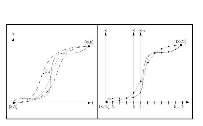
Figure 1: Representation of paths between $(x_{i},t_{i})$ and $(x_{f},t_{f})$, for the continuous case at the left (integral over continuum paths, see (1)) and for the discrete case at the right (integral over discrete paths before the continuum limit, see (4)). In the left figure, the continuous line is the classical path, the dashed lines are two paths obtained by variations around the classical paths and the dotted line is an arbitrary path. In the picture at the right the discrete path for fixed $n$ is shown together with the classical discrete path.

To understand this formula, we recall some ideas from Feynman’s thesis Feynman2 . Consider the particle at a point $x$ at time $t$. Suppose that the particle changes position by an amount $\delta x$ during an infinitesimal time interval $\delta t$. The action for this time interval can be written as $S[x+\delta,t+\Delta t;x,t]\simeq L[x,\frac{\delta x}{\delta t},t]\delta t$. We define the amplitude of transition between the states $|x,t\rangle$ and $|x+\delta x,t+\delta t\rangle$ as

$$\langle x+\delta x,t+\delta t|x,t\rangle\equiv\frac{1}{(2i\pi\hbar\epsilon/m)^{d/2}}e^{\frac{i}{\hbar}S[x+\delta x,t+\delta t,x,t]}\simeq\frac{1}{(2i\pi\hbar\epsilon/m)^{d/2}}e^{\frac{i}{\hbar}L[x,\frac{\delta x}{\delta t},t]\delta t}.$$

Then, if we divide the time interval $[t_{i},t_{f}]$ into a sequence of small intervals $t_{i}=t_{0}<t_{1}<t_{2}<\ldots<t_{n-1}<t_{f}=t_{n}$, where $t_{k}=t_{i}+k(t_{f}-t_{i})/n$, the transition amplitudes are multiplied (because successive events are independent):

$$\langle x_{f},t_{f}|x_{i},t_{i}\rangle=\langle x_{f},t_{f}|x_{n-1},t_{n-1}\rangle\ldots\langle x_{2},t_{2}|x_{1},t_{1}\rangle\langle x_{1},t_{1}|x_{i},t_{i}\rangle\ .$$

Integrating over all possible values of the intermediate positions $x_{k}$ leads to the formula (1), see Fig. 1. The intuition associated with this formula is as follows: we integrate the phase over all possible trajectories of the particle; unlike the classical case, the particle can follow paths that differ from the classical trajectory which minimizes the action. (Paths far away from the classical path usually make negligible contributions.) This image, though based on the classical image of a trajectory, illustrates the change in the mathematical description of the particle (wave-like behaviour) which can no longer be represented as a material point as its trajectory is not clearly defined with certainty.

The integral equation describing the evolution of the wave function $\Psi(x,t)$ (i.e. the state $|x,t\rangle$) over time, is given by

$$\Psi(x^{\prime},t^{\prime})=\int_{R^{d}}K(x^{\prime},t^{\prime};x,t)\Psi(x,t)dx\ .$$ (2)

It can be shown that the ‘wave function’ $\Psi(x,t)$ is also the solution of Schrödinger’s equation: $-\frac{\hbar^{2}}{2m}\Delta_{x}\Psi(x,t)+V(x,t)\Psi(x,t)=i\hbar\partial_{t}\Psi(x,t)$, where $\Delta_{x}$ is the $d$-dimensional Laplacian and $\partial_{t}\equiv\partial/\partial t$. For a proof of the equivalence between both formulations, see FH ,Feynman2 .

A useful example is the free particle amplitude calculation in one dimension. We simply replace the Lagrangian by the free Lagrangian, i.e. without potential, and use equation (1) to get :

$$K_{0}(x^{\prime},t^{\prime};x,t)=\frac{1}{\sqrt{2i\pi\hbar(t^{\prime}-t)/m}}e^{i\frac{m(x^{\prime}-x)^{2}}{2\hbar(t^{\prime}-t)}}\ .$$ (3)

Let us derive formula (3) starting from the general formula (1) applied to a free particle in 1-dimension. We divide the integral, for fixed $n$, we have to integrate the phase $e^{iS[x_{0},..,x_{n}]/\hbar}$ over the intermediate positions $x_{j},\ j=1,..,n-1$ at times $t_{j}=j\epsilon,\ \epsilon=(t_{f}-t_{i})/n$ between $x_{0}=x_{i}$ and $x_{n}=x_{f}$, where $S[x_{0},..,x_{n}]=\frac{m}{2}\sum_{j=1}^{n}\frac{(x_{j}-x_{j-1})^{2}}{\epsilon}$, multiplied by the constant $\left(\prod_{j=1}^{n}\sqrt{m/2i\pi\hbar\epsilon}\right)$. We need to calculate, for a fixed number of subdivision $n$, the multiple integral:

$$K_{0}^{(n)} (x_{n},t_{n};x_{0},t_{0})\equiv{}{}$$ (4)

$$\frac{1}{\sqrt{2i\pi\hbar\epsilon/m}}\int_{-\infty}^{\infty}\frac{dx_{1}}{\sqrt{2i\pi\hbar\epsilon/m}}\ldots\int_{-\infty}^{\infty}\frac{dx_{n-1}}{\sqrt{2i\pi\hbar\epsilon/m}}\exp{\left(i\sum_{j=1}^{n}(\frac{m(x_{j}-x_{j-1})^{2}}{2\hbar\epsilon})\right)}\ .$$

We perform the integration one stage at a time (from $j=1$ to $j=n-1$), using the well known formula for the convolution of two Gaussians. Given two Gaussians $g_{\sigma_{\nu}}(x)\equiv\frac{1}{\sqrt{2\pi\sigma_{\nu}^{2}}}e^{-\frac{x^{2}}{2\sigma_{\nu}^{2}}},\ \nu=1,2$, we have:

$$\int_{-\infty}^{\infty}g_{\sigma_{1}}(x-x^{\prime})g_{\sigma_{2}}(x^{\prime})=g_{\sqrt{\sigma_{1}^{2}+\sigma_{2}^{2}}}(x)\ .$$ (5)

Hence, in (4), we can calculate the integral with respect to $x_{1}$, changing variable to $x^{\prime}_{1}=x_{1}-x_{0}$, obtaining:

$$\frac{1}{\sqrt{2i\pi\hbar\epsilon/m}}\int_{-\infty}^{\infty}\frac{dx_{1}}{\sqrt{2i\pi\hbar\epsilon/m}}e^{i\frac{m(x_{2}-x_{1})^{2}}{2\hbar\epsilon}}e^{i\frac{m(x_{1}-x_{0})^{2}}{2\hbar\epsilon}}{}$$

$$= \frac{1}{\sqrt{2i\pi\hbar(2\epsilon)/m}}e^{i\frac{m(x_{2}-x_{0})^{2}}{2\hbar(2\epsilon)}}\ .$$

Proceeding by recursion, we get (4) :

$$K_{0}^{(n)}(x_{n},t_{n};x_{0},t_{0}) = \frac{1}{\sqrt{2i\pi\hbar(n\epsilon)/m}}e^{i\frac{m(x_{n}-x_{0})^{2}}{2\hbar(n\epsilon)}}\ ,$$

and hence (3) in the limit $n\rightarrow\infty$.

Clearly the 3-dimensional propagator is a product of 1-dimensional propagators:

$$K_{0}^{(3D)}(\overrightarrow{x}^{\prime},t^{\prime};\overrightarrow{x},t) = K_{0}(x^{\prime},t^{\prime};x,t)K_{0}(y^{\prime},t^{\prime};y,t)K_{0}(z^{\prime},t^{\prime};z,t){}$$ (6)

$$= \left(\frac{m}{2i\pi\hbar(t^{\prime}-t)}\right)^{3/2}e^{i\frac{m|\overrightarrow{x}^{\prime}-\overrightarrow{x}|^{2}}{2\hbar(t^{\prime}-t)}}\ ,$$

where $\overrightarrow{x}=(x,y,z)$ is the position vector in 3-dimensions. Note that for reasons to be discussed below, we shall not make use of the 3-dimensional propagator in the example of election diffraction for one and two slits. We remark for completeness, that the propagator (3) can be calculate by other methods, for example.Kleinert

III Application to the Problem of Electron Diffraction and Interference

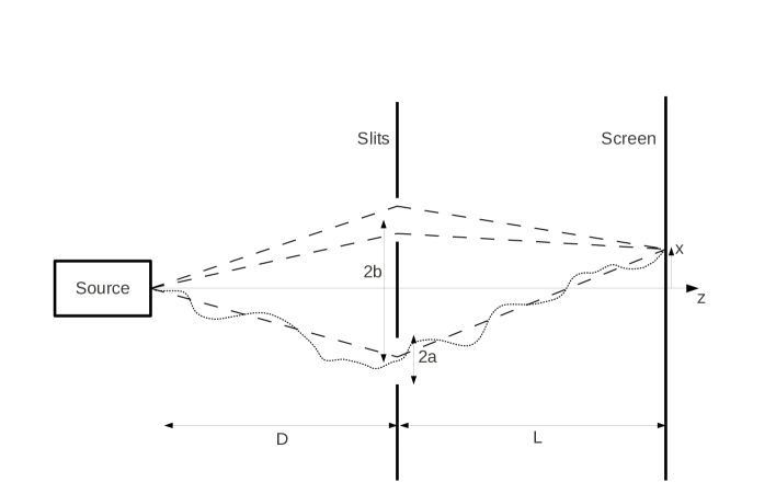
Figure 2: Schematic depiction of the apparatus with the source, the two-slits and the screen. We have represented four differents paths going through the slits, from the source to the screen. The dashed lines represent three classical paths and the thin dashed line a curved path. The Feynman path Integral formulation allows one to compute the propagator summing over all different paths, see equations (1), (3), (12), (16), (17), (18).

Consider an electron source at $(x,y,z)=(0,0,0)$, and two slits at $z=D$ of width $2a$ and centered respectively at $x=+b$ and $x=-b$, c.f. Fig. 2 . For the diffraction experiment with a single slit, just replace the system with a slit of size $2a$ centered at $x=0$. At $z=D+L$ is a screen on which electrons are recorded (or some other recording device). For more details about the experimental realization of the system, see Ref. Frabboni Note that we neglect gravity for this problem. In addition, we assume that in the direction orthogonal to the plane in Fig. 2 (the $x-z$-plane), the slot is long enough to neglect diffraction effects; we consider only the horizontal (in-plane) deflection of the beam in order not to complicate the formulas.

Then we can reduce the dimension of the propagator (6) by integrating over $y$:

$$K_{0}^{(2D)}(\overrightarrow{r}^{\prime},t^{\prime};\overrightarrow{r},t) = \int_{-\infty}^{\infty}dy\ K_{0}^{(3D)}(\overrightarrow{x}^{\prime},t^{\prime};\overrightarrow{x},t){}$$ (7)

$$= \frac{m}{2i\pi\hbar(t^{\prime}-t)}e^{i\frac{m|\overrightarrow{r}^{\prime}-\overrightarrow{r}|^{2}}{2\hbar(t^{\prime}-t)}}\ ,$$

where $\overrightarrow{r}=(x,z)$ is the position vector in the two dimensional plane orthogonal to the $y$-axis.

One can suggest different models for the slits given by distribution functions (e.g. Gaussian functions or ‘door’ functions). We focus on the more realistic model of ‘door’ functions (for the Gaussian function model, see Ref. FH ):

$$\chi_{[b-a,b+a]}(w)=\begin{cases}0&\text{$w>b+a,\ w<b-a$}\\ 1&\text{$b-a<w<b+a$}\end{cases}$$ (8)

The question is: what is the probability of finding the electron at the point $x$ on the screen knowing that it started at the point $(x=0,z=0)$? More precisely, suppose that the source emits electrons in large numbers, though small enough so that the distance between electrons is such that interactions can be neglected (no correlations). What is the intensity of electrons on the screen as a function of position $x$? The two questions are related since under these circumstances the motion of the electrons is independent (without mutual interaction, given that the density of the beam is very low). Indeed, the intensity curve is obtained by simply multiplying the probability curve for an electron by the number of electrons emitted per unit time. As explained above formula (1), the probability is given by the square of the amplitude which we will compute using the propagator (6).

As explained in (7), we now take $d=2$. In fact, we now argue that we can reduce the dimension further. For the $z$-direction, we really onght to use the two-dimensional propagator but we can reasonnably consider (as it is usually doneFrabboni ,FH ) that the propagator is a product of two independant propagator in both directions $x$ and $z$, where the last one is equal to a constant.

To see that, let us discuss the conceptual experiment for one slit.FH We consider that the problem is divided in two separate motions, one starting from the source to the slit during the time $T$ and the other one starting from the slit to the screen during the time $\tau$. Then, we would like to compute the probability amplitude for the electron from the source, at the intial position $(x=0,z=0)$ at the time $t=0$, to go to the screen, at the final position $(x,z=D+L)$ at the time $T+\tau$, knowing that it goes through the slit, at the intermediate position $(w,z=D),\ b-a<w<b+a$, at the time $t=T$. In fact, by the laws of quantum mechanics, there is no reasons to separate the motions in two independant parts, since we don’t know where is the particle at the time $T$.In other words we don’t know when the particle goes through the slit. Nevertheless, we can consider that this classical image is appropriated to study the problem. Indeed, the electron have in the $z$-direction the momentum $p_{z}=\hbar k_{z}$ ($k_{z}$ is the wave vector), which is related to the classical velocity $v_{z}=D/T=L/\tau$, where $D$ is supposed to be very large compared to the dimensions in the $x$-direction, more precisely, $x,a,b\ll D,L$. In addition we suppose that the wave lenght $\lambda$, which is approximatively equal to the $z$-direction wave lenght $\lambda\simeq\lambda_{z}=2\pi\hbar/(mv_{z})$, is small compared to the distances $\lambda\ll D,L$. Thus, the motion is approximatively classical in the $z$-direction and we can separate the problem as two independant motions. Notice that, quantum-mechanically, it is possible for the particle to go through the slit severals time before strike the screen,Yabuki but that the probability of this event is relatively small.

Now, let us compute the amplitude of the transition for the particle starting at the point $(x=0,z=0)$ at the time $t=0$, going through one slit at the position $(w,z=D),\ b-a<w<b+a$ at the time $t=T$ and arriving at the position $(x,z=L+D)$ at the time $t=T+\tau$:

$$K_{a,b}^{(2D)}((x,L+D),T+\tau; (0,0),0)\equiv\int_{-\infty}^{\infty}dw\ \chi_{[b-a,b+a]}(w)\times{}$$

$$K_{0}^{(2D)}\left((x,L+D),T+\tau;(w,D),\tau\right)K_{0}^{(2D)}\left((w,D),\tau;(0,0),0\right)\ .$$

Hence, the explicite formula is given by:

$$K_{a,b}^{(2D)}((x,L+D), T+\tau;(0,0),0)={}$$ (9)

$$\frac{e^{i\frac{mD^{2}}{2\hbar T}}}{\sqrt{2i\pi\hbar T/m}}\frac{e^{i\frac{mL^{2}}{2\hbar\tau}}}{\sqrt{2i\pi\hbar\tau/m}}\int_{b-a}^{b+a}dw\ \frac{e^{i\frac{m(x-w)^{2}}{2\hbar\tau}}}{\sqrt{2i\pi\hbar\tau/m}}\frac{e^{i\frac{mw^{2}}{2\hbar T}}}{\sqrt{2i\pi\hbar T/m}}\ .$$

Consequently, the two-dimensional propagator is the product of two independant one-dimensional propagators in the $x$ and in the $z$-directions, and since the propagator in $z$-direction is a constante (see the right hand sides of (9)):

$$K_{z}(L+D,T+\tau;0,0)=\frac{e^{i\frac{mD^{2}}{2\hbar T}}}{\sqrt{2i\pi\hbar T/m}}\frac{e^{i\frac{mL^{2}}{2\hbar\tau}}}{\sqrt{2i\pi\hbar\tau/m}}\ ,$$ (10)

we can reduce in the one-dimension’s $x$-direction the problem:

$$K_{x}(x,T+\tau;0,0)=\int_{b-a}^{b+a}dw\ \frac{e^{i\frac{m(x-w)^{2}}{2\hbar\tau}}}{\sqrt{2i\pi\hbar\tau/m}}\frac{e^{i\frac{mw^{2}}{2\hbar T}}}{\sqrt{2i\pi\hbar T/m}}\ .$$ (11)

Then we can reduce the dimension of the problem keeping only the $x$-axis propagator, as you can see in the ReferencesFH ,Frabboni . In the Reference,Frabboni they consider the slits in the $x$-$y$-plane, in two-dimensions and not in one-dimension as we do in the present article.

If we take the limit $a\rightarrow\infty$ (infinite slit), by (9) and by (5) we get:

$$K_{\infty}^{(2D)}((x,L+D),T+\tau;(0,0),0) = \frac{e^{i\frac{mD^{2}}{2\hbar T}}}{\sqrt{2i\pi\hbar T/m}}\frac{e^{i\frac{mL^{2}}{2\hbar\tau}}}{\sqrt{2i\pi\hbar\tau/m}}\int_{-\infty}^{\infty}dw\ \frac{e^{i\frac{m(x-w)^{2}}{2\hbar\tau}}}{\sqrt{2i\pi\hbar\tau/m}}\frac{e^{i\frac{mw^{2}}{2\hbar T}}}{\sqrt{2i\pi\hbar T/m}}{}$$

$$= \frac{e^{i\frac{mD^{2}}{2\hbar T}}}{\sqrt{2i\pi\hbar T/m}}\frac{e^{i\frac{mL^{2}}{2\hbar\tau}}}{\sqrt{2i\pi\hbar\tau/m}}\frac{e^{i\frac{mx^{2}}{2\hbar(T+\tau)}}}{\sqrt{2i\pi\hbar(T+\tau/m)}}\ .$$

Then we find the amplitude corresponding to the transition between the position $(x=0,z=0)$ at the time $t=0$ and the position $(x,z=L+D)$ at the time $t=T+\tau$, knowing that the position in the $z$-direction is $D$ at the time $t=T$ :

$$K_{\infty}^{(2D)}((x,L+D),T+\tau; (0,0),0){}$$

$$=K_{0,x}\left(x,T+\tau;0,0\right)K_{0,z}\left(L+D,T+\tau;D,\tau\right)K_{0,z}\left(D,T;0,0\right)\ ,$$

where $K_{o,X}(X^{\prime},t^{\prime};X,t)=(m/2i\pi\hbar(t^{\prime}-t))^{1/2}\exp{\left(im(X^{\prime}-X)^{2}/(2\hbar(t^{\prime}-t))\right)},\ X=x,z,$ are the 1-dimensional free propagators. Then, integrating over the intermediate positions $D$ between $-\infty$ and $+\infty$, we find the two dimensional free propagator (7) between $(x=0,z=0)$ at $t=0$ and $(x,z=L+D)$ at the time $t=\tau+T$:

$$\int_{-\infty}^{\infty}dD\ K_{\infty}^{(2D)} ((x,z=L+D),T+\tau;(0,0),0){}$$

$$=\int_{-\infty}^{\infty}dD\ \frac{e^{i\frac{mD^{2}}{2\hbar T}}}{\sqrt{2i\pi\hbar T/m}}\frac{e^{i\frac{m(z-D)^{2}}{2\hbar\tau}}}{\sqrt{2i\pi\hbar\tau/m}}\frac{e^{i\frac{mx^{2}}{2\hbar(T+\tau)}}}{\sqrt{2i\pi\hbar(T+\tau)/m}}\ ,{}$$

$$=\left(\frac{m}{2i\pi\hbar(T+\tau)}\right)e^{i\frac{m(x^{2}+z^{2})}{2\hbar(T+\tau)}}{}$$

$$=K_{0}^{(2D)}((x,z),T+\tau;(0,0),0)\ ,$$

to get the result, we have used the convolution formula between two Gaussians (5).

IV The exact result in terms of a Fresnel integral

Now we want to compute the amplitudes $A_{1}(x;a,b),\ A_{2}(x;a,b)$ at each point $x$ on the screen, using the Feynman formulation, and then to add both amplitudes to get the total amplitude $A(x;a,b)$ and finally to take the square of the modulus, obtaining the probability $P(x;a,b)\equiv|A(x;a,b)|^{2}$.

By (11), the formal expression for $A_{1}(x;a,b)$ is :

$$A_{1}(x;a,b)=\int_{-\infty}^{+\infty}dw\ \chi_{[b-a,b+a]}(w)K_{0}(x,T+\tau;w,T)K_{0}(w,T;0,0)\ ,$$ (12)

where $T$ is the travel time of the electron from the source to the slit and $\tau$ from the slit to the screen. Recall that to obtain formula (12), we used a similar argument to that which enabled us to write the formula (1), writing the integral over all possible paths as the product of independent amplitudes at successive times. However, in this case, at time $T$, we have to integrate over a finite interval (the slit), which results in the more complicated expression (12) rather than a Gaussian:

$$A_{1}(x;a,b)=\int_{b-a}^{b+a}dw\frac{1}{\sqrt{2i\pi\hbar\tau/m}}e^{i\frac{m(x-w)^{2}}{2\hbar\tau}}\frac{1}{\sqrt{2i\pi\hbar T/m}}e^{i\frac{mw^{2}}{2\hbar T}}\ .$$ (13)

Notice that :

$$\frac{m(x-w)^{2}}{2\hbar\tau}+\frac{mw^{2}}{2\hbar T}=(\frac{m}{2\hbar\tau}+\frac{m}{2\hbar T})(y-\frac{x}{1+\tau/T})^{2}+\frac{mx^{2}}{2\hbar(T+\tau)}\ ,$$

and hence,

$$A_{1}(x;a,b) = \frac{e^{i\frac{mx^{2}}{2\hbar(T+\tau)}}}{\sqrt{2i\pi\hbar(T+\tau)/m}}\int_{b-a}^{b+a}dw\sqrt{\frac{T+\tau}{2i\pi\hbar T\tau/m}}\exp{\left(i(\frac{T+\tau}{2\hbar T\tau/m})(w-\frac{x}{1+\tau/T})^{2}\right)}\ .{}$$ (14)

$$= \frac{e^{i\frac{mx^{2}}{2\hbar(T+\tau)}}}{\sqrt{(2i)^{2}\pi\hbar(T+\tau)/m}}\int_{\alpha_{-}^{(1)}(x)}^{\alpha_{+}^{(1)}(x)}dw^{\prime}\exp{\left(\frac{i\pi}{2}w^{\prime 2}\right)},$$

where

$$\alpha_{\pm}(x;a,b)\equiv\sqrt{\frac{(T+\tau)}{\pi\hbar T\tau/m}}(b\pm a)-\frac{x}{\sqrt{\pi\hbar\tau/m}}\sqrt{\frac{T}{T+\tau}}.$$ (15)

In (14), we see that we have the integral of a Gaussian with complex argument. Decomposing the integral in real and imaginary parts, we get two integrals of cosine and sine functions respectively, with second degree polynomial arguments. These integrals are the well-known Fresnel functions Abramowitz :

$$C[u]\equiv\int_{0}^{u}dw\cos{(\frac{\pi w^{2}}{2})}\ ,{}$$

$$S[u]\equiv\int_{0}^{u}dw\sin{(\frac{\pi w^{2}}{2})}\ .$$

Thus we obtain explicit analytical expressions for the amplitudes:

$$A_{1}(x;a,b) =\frac{e^{i\frac{mx^{2}}{2\hbar(\tau+T)}}}{\sqrt{(2i)^{2}\pi\hbar(T+\tau)/m}}\times{}$$ (16)

$$\big{(}C[\alpha_{+}(x;a,b)]-C[\alpha_{-}(x;a,b)]+iS[\alpha_{+}(x;a,b)]-iS[\alpha_{-}(x;a,b)]\big{)}\ ,$$

$$A_{2}(x;a,b) = A_{1}(x;a,-b)\ .$$ (17)

For two slits, we can compute the total amplitude by summing the amplitudes for both slits:

$$A(x;a,b)=A_{1}(x;a,b)+A_{2}(x;a,b)\ .$$ (18)

V Physical parameters, approximations and interpretations

Recall that the length of the slits and the distance between them is small compared to the horizontal distances $D$ and $L$, hence we can assume that the wave length of the electron $\lambda=h/mv$ is approximatively given by $h/mv_{z}$, where $v_{z}=L/\tau=D/T$. We will use this expression for the wave length in the following.

V.1 Diffraction by a single slit

We can write for the single-slit case (of size $2a$), the analogue of the function defined by (15):

$$\alpha(x;a)=\sqrt{N_{F}(a)}\sqrt{1+L/D}\left(1-\frac{x}{a}\frac{1}{1+L/D}\right)$$ (19)

where $N_{F}(a)=2a^{2}/\lambda L$ is the Fresnel number.

We can now easily compute the single-slit diffraction probability:

$$P^{(1Slit)}(x;a)=|A_{1}(x;a,b=0)|^{2}{}$$ (20)

$$= \frac{1}{2\lambda(L+D)}\left([C(\alpha(x;a))+C(\alpha(x;-a))]^{2}+[S(\alpha(x;a))+S(\alpha(x;-a))]^{2}\right)\ .$$

Let us introduce the following parameters $\eta\equiv 1+L/D$ and $\gamma=\eta-1$. We can then plot the functions (20) for various values of these parameters, see Fig 3. Note that the Fresnel functions in (20) behave differently depending on the value of the Fresnel number $N_{F}(a)$, esp. depending on whether it is greater or less than unity. To understand these differences explicitly, we will analyse the asymptotic behavior of these functions for different regimes of $N_{F}(a)$ using the known asymptotics of the Fresnel functions: (see Abramowitz )

$$C(\pm u)\simeq\ \pm\frac{1}{2}+\frac{1}{\pi u}\sin{\frac{\pi u^{2}}{2}}\ ,\ u\gg 1\ ,{}$$

$$S(\pm u)\simeq\ \pm\frac{1}{2}-\frac{1}{\pi u}\cos{\frac{\pi u^{2}}{2}}\ ,\ u\gg 1\ .$$ (21)

If we have:

$$\frac{x}{a\eta}-1\gg\frac{1}{\sqrt{N_{F}(a)\eta}}\ ,$$

we get the asymptotic behavior for the functions defined by (19):

$$\alpha(x;a)\ll-1\ \mathrm{and}\ \alpha(x;-a)\gg 1\Leftrightarrow\pm\alpha(x;\mp a)\gg 1\ ,$$ (22)

and so by (V.1) and (22), the asymptotics formulas of the Fresnel functions in (20) are given by:

$$C[\alpha(x;\pm a)]\simeq\pm\frac{1}{2}+\frac{1}{\pi\alpha(x;\pm a)}\sin{(\frac{\pi\alpha(x;\pm a)^{2}}{2})},{}$$

$$S[\alpha(x;\pm a)]\simeq\pm\frac{1}{2}-\frac{1}{\pi\alpha(x;\pm a)}\sin{(\frac{\pi\alpha(x;\pm a)^{2}}{2})}\ .$$ (23)

Then we get:

$$C[\alpha(x;+a)]+C[\alpha(x;-a)]\simeq\frac{1}{\pi\alpha(x;a)}\sin{(\frac{\pi\alpha(x;a)^{2}}{2})}+\frac{1}{\pi\alpha(x;-a)}\sin{(\frac{\pi\alpha(x;-a)^{2}}{2})},{}$$

$$S[\alpha(x;+a)]+S[\alpha(x;-a)]\simeq\frac{-1}{\pi\alpha(x;a)}\cos{(\frac{\pi\alpha(x;a)^{2}}{2})}-\frac{1}{\pi\alpha(x;-a)}\cos{(\frac{\pi\alpha(x;-a)^{2}}{2})}$$ (24)

Applying the Fresnel function asymptotic forms (V.1) to (20) and using the definition (19), we deduce than if $N_{F}(a)\ll 1$ and if $(x-a\eta)/a\eta\gg 1/\sqrt{N_{F}(a)\eta}\Leftrightarrow x-a\eta\gg\sqrt{\lambda L/2}$, we get the following asymptotic formula:

$$P^{(1Slit)}(x;a) \simeq \frac{2\gamma}{\pi^{2}\eta^{2}}\left(\frac{a^{2}}{(\frac{x^{2}}{\eta^{2}}-a^{2})^{2}}+\frac{1}{\frac{x^{2}}{\eta^{2}}-a^{2}}\sin^{2}{(\pi N_{F}(a)\frac{x}{a})}\right)\ ,$$ (25)

Moreover, since $N_{F}(a)\ll 1$ and so $\frac{x}{a\eta}\gg 1$, we have another asymptotic form (large distance on the screen):

$$P^{(1Slit)}(x;a) \simeq \frac{2\gamma}{\pi^{2}x^{2}}\sin^{2}{(\pi N_{F}(a)\frac{x}{a})},\ (N_{F}(a)\ll 1,\ x/a\eta\gg 1)\ ,$$ (26)

In this case we are in the so-called Fraunhofer regime analogous to plane wave diffraction in optics.Optics In fact, notice that the distance between fringes is $a/N_{F}(a)=\lambda_{z}L/2a$, c.f. Fig 3a.

Both approximations (25) and (26) are also valid if $N_{F}(a)$ is of the order of unity (this is the intermediate regime) provided that $x\gg a\eta$. This means that the pattern on the screen far from the position of the first lobe is well approximated by equations (25) and (26), see Fig. 3b.

On the contrary, if $N_{F}(a)\gg 1$, we get different asymptotics given by:

$$P^{(1Slit)}(x)\simeq\frac{\gamma}{\eta}\left(\frac{\sqrt{N_{F}(a)}}{2a}+\frac{\sin{(\frac{\pi}{2}N_{F}(a)\eta(1-\frac{x}{a\eta})^{2})}}{2\pi\sqrt{\eta}(a-\frac{x}{\eta})}+\frac{\sin{(\frac{\pi}{2}N_{F}(a)\eta(1+\frac{x}{a\eta})^{2})}}{2\pi\sqrt{\eta}(a+\frac{x}{\eta})}\right)^{2}{}$$ (27)

$$+ \frac{\gamma}{\eta}\left(\frac{\sqrt{N_{F}(a)}}{2a}-\frac{\cos{(\frac{\pi}{2}N_{F}(a)\eta(1-\frac{x}{a\eta})^{2})}}{2\pi\sqrt{\eta}(a-\frac{x}{\eta})}-\frac{\cos{(\frac{\pi}{2}N_{F}(a)\eta(1+\frac{x}{a\eta})^{2})}}{2\pi\sqrt{\eta}(a+\frac{x}{\eta})}\right)^{2},\ |x|<a\eta,$$

$$P^{(1Slit)}(x) \simeq\frac{2\gamma}{\pi^{2}\eta^{2}}\left(\frac{a^{2}}{(\frac{x^{2}}{\eta^{2}}-a^{2})^{2}}+\frac{1}{\frac{x^{2}}{\eta^{2}}-a^{2}}\sin^{2}{(\pi N_{F}(a)\frac{x}{a})}\right),\ |x|>a\eta\ ,$$ (28)

since the asynptotic behavior of the functions (19) are:

$$\alpha(x;\pm a)\gg 1,\ \mathrm{if}\ N_{F}(a)\gg 1\ \mathrm{and}\ |x|<a\eta\ ,{}$$ (29)

$$\pm\alpha(x;\mp a)\gg 1,\ \mathrm{if}\ N_{F}(a)\gg 1\ \mathrm{and}\ |x|>a\eta\ ,$$ (30)

so if $|x|<a\eta$, by (29) and (V.1), we get:

$$C[\alpha(x;\pm a)]\simeq\frac{1}{2}+\frac{1}{\pi\alpha(x;\pm a)}\sin{(\frac{\pi\alpha(x;\pm a)^{2}}{2})},{}$$

$$S[\alpha(x;\pm a)]\simeq\frac{1}{2}-\frac{1}{\pi\alpha(x;\pm a)}\sin{(\frac{\pi\alpha(x;\pm a)^{2}}{2})}\ ,$$ (31)

then by (29) and (V.1), we have:

$$C[\alpha(x;+a)]+C[\alpha(x;-a)]\simeq 1+\frac{1}{\pi\alpha(x;a)}\sin{(\frac{\pi\alpha(x;a)^{2}}{2})}+\frac{1}{\pi\alpha(x;-a)}\sin{(\frac{\pi\alpha(x;-a)^{2}}{2})},{}$$

$$S[\alpha(x;+a)]+S[\alpha(x;-a)]\simeq 1-\frac{1}{\pi\alpha(x;a)}\cos{(\frac{\pi\alpha(x;a)^{2}}{2})}-\frac{1}{\pi\alpha(x;-a)}\cos{(\frac{\pi\alpha(x;-a)^{2}}{2})}\ ,$$

then we get (27).

If $|x|>a\eta$, by (30) and (V.1), we get the same approximations as (V.1) and (V.1), then we obtain (28).

Note that the function (27) oscillates rapidly in the interval $[-a,+a]$ (esp. near the edges) around a constant value $N_{F}(a)\gamma/2a^{2}\eta=1/(\lambda_{z}(L+D))$, whereas for $|x|>a\eta$, the function (28) decreases rapidly to $0$. Hence $P^{(1Slit)}$ tends at large $N_{F}(a)$ to the ‘door’ function defined by (8), as might have been expected, see Fig. 3c.

Figure 3: Diffraction curve for a single-slit, with $\eta=2$. The abscissae are the distances in units of $a$ and the ordinates are the relative populations. We have $N_{F}(a)=0.01$ for the Figure (3a), $0.5$ for (3b), and $100$ for (3c).

V.2 Comment about the probability interpretation

We can see that (20) has the physical dimension of the inverse of a length squared and so it is neither a probability nor a probability density. This apparent problem can, however, be seen to be a matter of interpretation by looking at the formula (2). Indeed, the probability density for the diffraction problem is given by $|\Psi(x,T+\tau)|^{2}$, where $\Psi(x,T+\tau)$ is a normalized wave function, i.e. $\int_{R^{1}}dx\,|\Psi(x,T+\tau)|^{2}=1$. Therefore, we must choose an initial wave function (at time $t=0$) which is also normalized so that its square modulus describes the probability distribution of the electron in the $x_{0}$ plane. Essentially, what we have done in (20) is to take the initial wave function to be a delta-function, whereas it should be the initial probability distribution which is a delta-function, i.e. $\Psi(x,0)$ should be ‘the square root of a delta-function’.

To make this clearer, consider for example a wave function at time $t=0$ given by the square root of a Gaussian $\phi_{\sigma}(x_{0})=\frac{1}{(2\pi\sigma^{2})^{1/4}}e^{-\frac{x_{0}^{2}}{4\sigma^{2}}}$, so that $\int_{R^{1}}dx_{0}\,|\phi_{\sigma}(x_{0})|^{2}=1$ and $|\phi_{\sigma}(x_{0})|^{2}\rightarrow\delta(x_{0})$ as $\sigma\rightarrow 0$. In this way the wave function obtained in (34) is properly normalized so as to get the probability of the presence of the electron at the point $x$ on the screen by taking the square of the modulus. Indeed, the wave function at time $t=T$, i.e. at the position of the slits, is given by:

$$\phi_{\sigma}(x,T)=\int_{R^{1}}dx_{0}\,K_{0}(x,T;x_{0},0)\phi_{\sigma}(x_{0})\ ,$$ (32)

where $K_{0}(x,T+\tau;x_{0},0)$ is the free propagator defined by the equation (3). Using the identity

$$\int_{R^{1}}K_{0}(x,T;x_{0},0)^{*}K_{0}(x,T;x_{0}^{\prime},0)dx=\delta(x_{0}-x_{0}^{\prime})$$ (33)

we have that $\phi_{\sigma}(x,T)$ remains normalized, i.e. $\int|\phi_{\sigma}(x,T)|^{2}dx=1$.

The wave function at time $t=T+\tau$ is given by:

$$\Psi_{\sigma}(x,T+\tau)=\int_{-a}^{+a}dyK_{0}(x,T+\tau;y,T)\phi_{\sigma}(y,T).$$ (34)

Now, the quantity of interest is the conditional probability (density) for the electron to be at the point $x$ on the screen at the time $T+\tau$ given that it was in the interval $[-a,+a]$ at time $T$, i.e. given that it passed through the slit:

$$P_{\sigma}\left(x,T+\tau\,|\,y\in[-a,+a],T\right)\equiv\frac{|\Psi_{\sigma}(x,T+\tau)|^{2}}{\int_{-a}^{+a}dy\,|\phi_{\sigma}(y,T)|^{2}}\ .$$ (35)

after which we wish to take the limit $\sigma\rightarrow 0$. Using the relation (33) one can see that the condition probability (35) is normalized so that this procedure just amounts to division by a normalization factor. Thus

$$\int_{R^{1}}dx\,|\Psi_{\sigma}(x,T+\tau)|^{2}=\int_{-a}^{+a}dy|\phi_{\sigma}(y,T)|^{2}\ .$$ (36)

To take the limit $\sigma\to 0$, note that $\phi_{\sigma}(x_{0})=(8\pi\sigma^{2})^{1/4}g_{\sigma\sqrt{2}}(x_{0})$ where $g_{\sigma\sqrt{2}}(x_{0})=\frac{e^{-\frac{x_{0}^{{}^{\prime}2}}{4\sigma^{2}}}}{\sqrt{4\pi\sigma^{2}}}$ is a normalized Gaussian of variance $\sigma\sqrt{2}$, and hence $g_{\sigma\sqrt{2}}(x_{0})\rightarrow\delta(x_{0}),\ \sigma\rightarrow 0$. Multiplying top and bottom of (34) by $(8\pi\sigma^{2})^{1/2}$ we thus have

$$\lim_{\sigma\rightarrow 0} P_{\sigma}\left(x\in A,T+\tau|y\in[-a,+a],T\right)={}$$ (37)

$$=\lim_{\sigma\rightarrow 0}\frac{(8\pi\sigma^{2})^{-1/2}|\Psi_{\sigma}(x,T+\tau)|^{2}}{(8\pi\sigma^{2})^{-1/2}\int_{-a}^{+a}dy|\phi_{\sigma}(y,T)|^{2}}\ ,{}$$

$$=\frac{\left|\int dx_{0}K(x,T+\tau;x_{0},0)g_{\sigma\sqrt{2}}(x_{0})\right|^{2}}{\int_{-a}^{a}dy\,\left|\int dx_{0}K_{0}(y,T;x_{0},0)g_{\sigma\sqrt{2}}(x_{0})\right|^{2}}{}$$

$$=\frac{|K(x,T+\tau;0,0)|^{2}}{\int_{-a}^{+a}dy|K_{0}(y,T;0,0)|^{2}}{}$$

$$=\frac{\lambda L}{2a}P^{1Slit}(x;a)\ ,$$

where

$$K(x,T+\tau;0,0)=\int_{-a}^{+a}dy\,K_{0}(x,T+\tau;y,T)K_{0}(y,T;0,0)$$ (38)

is the propagator through the slit and $P^{(1Slit)}(x;a)=|K(x,T+\tau;0,0)|^{2}$ is given by (20). Note that this now has the correct dimension of an inverse length.

V.3 Interference and diffraction for two slits

Similarly, one can find the two-slit diffraction probability formula using (16), (17) :

$$P^{(2Slit)}(x;a,b) = P_{1}(x;a,b)+P_{2}(x;a,b)+I_{12}(x;a,b)\ ,$$ (39)

with the diffraction terms :

$$P_{1}(x;a,b)=|A_{1}(x;a,b)|^{2}{}$$ (40)

$$= \frac{\gamma}{2\lambda L\eta}\left([C(\alpha_{+}(x;a,b))-C(\alpha_{-}(x;a,b))]^{2}+[S(\alpha_{+}(x;a,b))-S(\alpha_{-}(x;a,b))]^{2}\right)\ ,{}$$

$$P_{2}(x;a,b)=|A_{2}(x;a,b)|^{2}=P_{1}(x;a,-b)\ ,$$

and the interference term :

$$I_{12}(x;a,b) = A_{1}(x;a,b)A_{2}(x;a,b)^{*}+A_{2}(x;a,b)A_{1}(x;a,b)^{*}{}$$ (41)

$$= \frac{\gamma}{\lambda L\eta}([C(\alpha_{+}(x;a,b))-C(\alpha_{-}(x;a,b))][C(\alpha_{+}(x;a,-b))-C(\alpha_{-}(x;a,-b))]{}$$

$$+ [S(\alpha_{+}(x;a,b))-S(\alpha_{-}(x;a,b))][S(\alpha_{+}(x;a,-b))-S(\alpha_{-}(x;a,-b))])\ .$$

Notice that there is an additional term compared to the single-slit case called the interference term, which is of course quite similar to that in optics.Optics This results in a modulation effect of the curve given by (39) by the sum of the diffraction terms (40) (modulo a multiplicative factor), see Fig. 4.

Let us define the Fresnel numbers

$$N_{F}(a)\equiv 2a^{2}/\lambda_{z}L,\quad N_{F}(b)\equiv 2b^{2}/\lambda_{z}L\mbox{ and }N_{F}\equiv 2ab/\lambda_{z}L=\sqrt{N_{F}(a)N_{F}(b)/2}.$$

Assume that the distance between the slits is large compared to the size of the slits $b\gg a$. In the experiment considered one fixes both parameters $a$ and $b$ and varies the distance between the screen and the slits (keeping the same value for $\eta$). Notice that because $b\gg a$, $N_{F}\gg 1$ does not necessarily imply that $N_{F}(a)\gg 1$. Thus we will see that both parameters play different roles.

First, we establish the asymptotics of (39) for different asymptotic value of $N_{F}(a)$. Under the condition $N_{F}(a)\ll 1$ and at large scales $|x-b\eta|\gg a\eta$ et $|x+b\eta|\gg a\eta$, we get similar expressions for $P_{1}(x;a,b)$ and $P_{2}(x;a,b)$ as (26). We have to compute the asymptotic expression for the interference term. This yields

$$P^{(2Slit)}(x;a,b) \simeq \frac{2\gamma}{\pi^{2}(x-b\eta)^{2}}\sin^{2}{\left(\pi N_{F}\eta(1-\frac{x}{b\eta})\right)}+\frac{2\gamma}{\pi^{2}(x+b\eta)^{2}}\sin^{2}{\left(\pi N_{F}\eta(1+\frac{x}{b\eta})\right)}{}$$ (42)

$$- \frac{\gamma}{\pi^{2}(x^{2}-b^{2}\eta^{2})}\left(\cos{(2\pi(N_{F}+N_{F}(a))\frac{x}{a})}-\cos{(2\pi N_{F}\eta(1+\frac{x}{a\eta}))}\right){}$$

$$- \frac{\gamma}{\pi^{2}(x^{2}-b^{2}\eta^{2})}\left(\cos{(2\pi(N_{F}-N_{F}(a))\frac{x}{a})}-\cos{(2\pi N_{F}\eta(1-\frac{x}{a\eta}))})\right)\ .$$

One can observe that there are two phases: the separated phase ($N_{F}\gg 1$) and the mixed phase ($N_{F}\ll 1$). At the same time there are the Fresnel and Fraunhofer regimes depending on the values of $N_{F}(a)$ as explained above. The distinction between two phases is purely geometric and characterizes the separation respectively mixture of diffraction curves. Indeed, similar to optics, to observe the two diffraction curves separately, the fringe modulation $\lambda_{z}L/2a$ must be less than the distance between the origins of the two curves (being centered in $\pm b\eta$) because otherwise both curves are mixed. Thus the criterion is written $\lambda_{z}L/2a<b\eta$ and therefore $N_{F}\eta>1$. This obviously unlike the case $N_{F}\ll 1$ where the two curves are combined (one added to the other) and where we observe modulation interference.

To see this more formally, consider firstly the case $N_{F}\eta\ll 1$. If $|x|>\lambda L/2a$ then $|x|\gg b\eta$ and we can give an approximation of (42). Indeed, the first two terms are approximately equal and contribute

$$\frac{4\gamma}{\pi^{2}x^{2}}\sin^{2}(\frac{2\pi a}{\lambda L}x).$$

In the last two terms we develop the cosine functions and get

$$2\left[\cos{(\frac{2\pi b}{\lambda L}x)}\cos{(\frac{2\pi a}{\lambda L}x)}-\cos{(\frac{2\pi ab\eta}{\lambda L})}\cos{(\frac{2\pi b}{\lambda L}x)}\right]$$

$$\approx-4\cos(\frac{2\pi b}{\lambda L}x)\sin^{2}(\frac{2\pi a}{\lambda L}x),$$

where we used $\cos{(\frac{2\pi ab\eta}{\lambda L})}\simeq 1$ because $N_{F}\eta\ll 1$. Adding the terms we obtain

$$P^{(2slit)}(x;a,b)\simeq\frac{8\gamma}{\pi^{2}x^{2}}\sin^{2}{(\frac{2\pi a}{\lambda L}x)}\cos^{2}{(\frac{2\pi b}{\lambda L}x)}\ .$$ (43)

This is the familiar optical formula: see Reference,Optics formula (10) Chap. VIII-6. It shows that the diffraction curves are modulated by interference fringes. The distance between two interference fringes is of the order of $\lambda_{z}L/2b$ whereas that between minima of the diffraction curves is of the order of $\lambda_{z}L/2a\gg\lambda_{z}L/2b$, see Fig. 4a, Fig. 4b (far from the first lobe) and Fig. 4c.

Secondly, consider the case that $N_{F}\eta\gg 1$ (while still assuming $N_{F}(a)\ll 1$). If $x-b\eta>-\lambda L/2a$ (or $x+b\eta<\lambda L/2a$) then $(x-b\eta)^{-2}\gg(x+b\eta)^{-2}$ (respectively $(x-b\eta)^{-2}\ll(x+b\eta)^{-2}$) so one of the two terms is negligible in the respective domain. Moreover, in both cases, the interference term is small compared to the diffraction term since $(x-b\eta)^{-2}\gg(x^{2}-b^{2}\eta^{2})^{-1}$. The total probability is therefore approximatively equal to a sum of the two diffraction curves centered at $\pm b\eta$ modulated by an interference term which oscillates rapidly with a relatively small amplitude, c.f. Fig 4c :

$$P^{(2slit)}(x;a,b) \simeq \frac{2\gamma}{\pi^{2}(x\mp b\eta)^{2}}\sin^{2}\left(\pi N_{F}\eta(1\mp\frac{x}{b\eta})\right)+O(\frac{1}{x^{2}-b^{2}\eta^{2}}),\ |x\pm b\eta|>\frac{\lambda L}{2a}\ .$$ (44)

Now, consider $N_{F}(a)\gg 1$. Since, unlike the previous cases, we do not need special conditions for the position $x$ on the screen, we find similar formulas to (27) and (28) for the direct terms $P_{1}$ and $P_{2}$, except that $x$ is replaced by $x-b\eta$ for the slit centered at $+b$ and by $x+b\eta$ for the slit centered at $-b$.

For the interference term, inserting the asymptotics (V.1) into (41) above results in the sum of two terms, one being the product of differences of cosin-functions, the other the product of differences of sin-functions. The problem is obviously symmetric about $x=0$, so we need only consider the case $x>0$. Then there are again two cases:
(i) $|x-b|>a$; and (ii) $|x-b|<a$.
In the first case, both terms decrease like $1/(x+b)(x-b)$ with various fluctuating factors as in (42). In the second case, $P_{1}$ behaves as in (27) but centred around $x=b$, and the other terms are negligible. We do not write the asymptotic formulas explicitly because the result is simply the observation that in this case we obtain a sum of two separated diffraction curves in the Fresnel regimes, i.e. curves that tend to the door functions in the limit, see Fig. 4d.

Notice an interesting behavior of the interference pattern in Fig. 4c, where we see that the interference amplitudes are very small compared to the diffraction amplitude inside a band $25{<\atop\sim}|x/a|{<\atop\sim}75$, so that there are no interference fringes. This is also discernible in Fig. 4b of the ReferenceFrabboni which corresponds to the calculated two-slit diffraction images, where one can observe the absence of fringes in a band. However, this phenomenon is not apparent on the corresponding experimental image. This is probably due to the difference in defocussing between the calculated and experimental images, see Fig. 3b and Fig. 4b of the Reference.Frabboni Indeed, the existence of such a band is quite sensitive to the value of the parameter $N_{F}(a)$.

Figure 4: Interference curves $(\ref{P2})$ from two slits, with $b/a=13,\ \eta=2$. The abscissae are the distances in units of $a$ and the ordinates are the relative populations. We have $N_{F}(a)=0.001$ for the Figure (4a) , $0.015$ for (4b), $0.12$ for (4c) and $6$ for (4d).

VI Conclusion and remarks

- We have briefly presented the Feynman approach to quantum mechanics, based on the Lagrangian formulation of classical mechanics, and the associated change in paradigm in the transition from classical to quantum mechanics. We note that in this approach, the transition from classical to quantum mechanics is quite natural because it relies mostly on concepts well known to students of analytical mechanics and does not confuse particle and wave behavior. It thus avoids some metaphysical questions and leads directly to the solution of the diffraction and interference problems above, and hence to a better understanding of the quantum mechanics of such quintessential phenomena. This justifies introducing the Feynman formulation at an early stage especially as the semi-classical approach that is often used in a first course relies on the idea of quantification of the action. A parallel introduction of the Feynman integral thus makes sense as it clarifies the passage classical to quantum.

- Secondly, it seemed of interest to derive explicit formulas for the problem of diffraction / interference by one or two slits, and to discuss the results based on the physical parameters of the system, notably the Fresnel numbers and the distance scale at which we observe on the screen. The properties of the diffraction and interference patterns are not apparent from the exact formulas (20) (39), so it is useful to establish asymptotic forms (25) (26) (27) for the case of one slit, and (42) for the case of two slits.

We summarize the various conclusions. In case of a single slit:

- If $N_{F}(a)\ll 1$, this is the Fraunhofer regime for which the distribution curve is similar to the plane wave case, c.f. equations (25), (26) and Fig. 3a.

- If $N_{F}(a)\gg 1$, this is the Fresnel regime for which the diffraction curve approximates the form of the slit, c.f. equations (27), (28) and Fig. 3c.

- If $N_{F}(a)\sim 1$ one is in the intermediate regime for which there is a spreading around the center of the electronic distribution and we find the case of Fraunhofer distances on the screen, c.f. equation (20) and Fig. 3b.

In the case of two slits of width $2a$, and separated by a distance $2b$ with $b\gg a$, we can make similar distinctions as in the one-slit diffraction case but there is also a transition between two phases dependent on the optical resolution:

- If $N_{F}\ll 1$, one is in the mixed phase, i.e. we observe an interference curve modulated by a diffraction curve for a slit of size $a$ in this case $N_{F}(a)\ll 1$, then we are in the regime of Fresnel, c.f. equations (42), (43) and Fig. 4a.

- If $N_{F}\gg 1$, one is in the separated phase, and there are two interference curves (the interference amplitudes are lower) modulated by the diffraction curves corresponding to both slits, each curve being centered respectively at $\pm b\eta$; the shapes of the diffraction curves modulating the signals of each of the slits depends on $N_{F}(a)$ and are similar to the case of a single slit as summarized above (with three regimes: Fresnel, Fraunhofer and intermediate), c.f. (44), Fig. 4c for $N_{F}(a)\ll 1$ and Fig. 4d for $N_{F}(a)\gg 1$.

- If $N_{F}\sim 1$ we observe a separation between two interference curves, modulated by the diffraction curve corresponding to one slit at the intermediate regime. see Fig. 4b and Eq. (42).

Note that the fringes corresponding to the diffraction are at a distance $\lambda L/2a$ and those for interference at about $\lambda L/2b$. The analytical properties of our asymptotics of two slits do not permit us to estimate these distances more exactly, but by analogy with optics they may be considered adequate.

In perspective, I suggest to take into account the quantum-mechanical way in the $z$-direction to solve the problem completely. Indeed, recall that as we discussed in the Section III, we consider in this article that the problem is separated in two motions, one between the source and the slits and the other one between the slits and the screen, which is rigorously not true. This is a challenging task since we have also to compute the loop path corrections,Yabuki but it could be an interesting contribution to the European Journal of Physics.

References

References

• (1) R. P. Feynman, R. B. Leighton, and M. L. Sands , The Feynman Lectures on Physics (Addison-Wesley, Reading, MA, 1963).
• (2) R. P. Feynman and A. R. Hibbs, Quantum Mechanics and Path Integrals (New York: McGraw-Hill), 3rd. ed. (1965)
• (3) C. Jönsson, “Elektroneninterferenzen an mehreren künstlich hergestellten Feinspalten“, Z. Phys. 161 (4), 454-474 (1961).
• (4) Anton Zeilinger et al, ”Single- and double-slit diffraction of neutrons”, Rev. Mod. Phys. 60, 1067-1073 (1988)
• (5) R. L. Pfleegor and L. Mandel, ”Interference of Independent Photon Beams”, Phys.Rev 159 (5), 1084-1088 (1967).
• (6) M. Abramowitz and I. A. Stegun, Handbook of Mathematical Functions, (Dover, New York, 1965).
• (7) Stefano Frabboni et al, “Two and three slit electron interference and diffraction experiments,” Am. Journ. Phys. 79 (6), 615–618 (2011).
• (8) A. O. Barut and S. Basri, ”Path integrals and quantum interference”, Am. J. Phys. 60, 896-899 (1992).
• (9) M. Fanaro, M. Arlego, M. R. OTERO, “A Didactic Proposed for Teaching the Concepts of Electrons and Light in Secondary School Using Feynman´s Path Sum Method”, European J of Physics Education 3:2, 1-11 (2012)
• (10) R. P. Feynman, Feynman’s Thesis: A New Approach to Quantum Theory, edited by Laurie M. Brown (World Scientific, Singapore, 2005).
• (11) R. P. Feynman, “Space-time approach to non-relativistic quantum mechanics,” Rev. Mod. Phys. 20, 367-387 (1948).
• (12) H. Kleinert, Path Integrals in Quantum Mechanics, Statistics, Polymer Physics, and Financial Markets (World Scientific Publishing Co., Singapore, 4th edition, pp. 1- 1547, 2006).
• (13) H. Yabuki, ”Feynman Path Integrals in the Young Double-Slit Experiment”, Int. J. Theor. Phys 25:2, 159-174 (1986)
• (14) M. Born and E. Wolf, Principles of Optics: Electromagnetic Theory of Propagation, Interference and Diffraction of Light, 4th ed. (Pergamon, Oxford, 1969).