FLRW cosmology in Weyl-Integrable Space-Time

Abstract

We investigate the Weyl space-time extension of general relativity (GR) for studying the FLRW cosmology through focusing and defocusing of the geodesic congruences. We have derived the equations of evolution for expansion, shear and rotation in the Weyl space-time. In particular, we consider the Starobinsky modification, $f(R)=R+\beta R^{2}-2\Lambda$, of gravity in the Einstein-Palatini formalism, which turns out to reduce to the Weyl integrable space-time (WIST) with the Weyl vector being a gradient. The modified Raychaudhuri equation takes the form of the Hill-type equation which is then analysed to study the formation of the caustics. In this model, it is possible to have a Big Bang singularity free cyclic Universe but unfortunately the periodicity turns out to be extremely short.

I Introduction

In order to solve the problems (viz. singularity, flatness, horizon) concerning the early universe in cosmology, the modification of the classical geometrical structure of General Relativity (GR) becomes pertinent and various such modifications are attempted time and again Hawking:1973uf ; Wald:1984rg ; Joshi:1987wg ; Ellis:1971pg ; Carroll:1997ar . Various inflationary cosmological models Tasi , scalar-tensor theories and the models resulting from the string theory Fujii:2003pa such as dilaton gravity are considered to solve the above-mentioned problems which are still not satisfactorily answered. These modifications amount in general to introducing a scalar field for some models while for others they appeal to a unified description of the fundamental forces for understanding cosmology of the early universe Albrecht:1982wi . In the context of unification of the forces, the Weyl space-time through its non-metric connection with a vector field $(W_{\mu})$ could facilitate unification of the two long range forces, electromagnetic and gravity.

The field $W_{\mu}$ defines an enlarged structure of space-time namely the Weylian manifold. The Weyl extension is a natural generalized space-time structure if we employ light rays and freely falling observers instead of clocks clock , Ehlers as the basic tools for maping the space-time. the EPS axiomatization shown Ehlers that Weyl space-time is the natural structure if we use light rays and freely falling particles instead of clocks as basic tools. In this approach, the Riemannian geometry is replaced by a Weyl geometry as the structure of the space-time which enlarges the framework of the GR space-time and as a direct consequence, a purely geometric fundamental new field is introduced into the theory of gravitation. The characterisation of the space-time and geodesic congruences with Weyl geometry in the Einstein-Palatini formalism need to be considered carefully for the complete manifestation of the gravitational fields Poulis:2011ve ; Fatibenea:2011aw .
The formation of caustics Poisson ; Anirvan in a given space-time is important to examine the singularities of the space-time foliations Joshi:1987wg ; Sardanashvily . The caustics is an undesirable feature as it indicates failure of proper evolution of physical fields in certain region of space-time Felder ; Goswami . A caustic is therefore a singularity of a geodesic congruence where the equation of motion becomes untenable at such points Poisson . The study of the formation of caustics in the field configuration relative a given space-time background is therefore very important and the analysis of the Raychaudhuri equation Poisson ; Sayan1 ; Dadhich in diverse various settings Anirvan ; Anirvan1 plays a crucial role in probing the physical viability of a model in relation to the occurrence of the space-time singularities Joshi:1987wg ; Goswami .

In the present paper, we study the formation of caustics by examining focusing and defocusing of geodesic congruences in the Weyl space-time which becomes WIST for $f(R)$ gravity in the Einstein-Palatini formalism. It is then equivalent to a conformal transformation. One of the basic tools of analysis is however the Raychaudhuri equation. The paper is organized as follows: In the next section, we set up the Weyl space-time structure which is followed by the computation of the kinematic parameters namely expansion scalar, shear and rotation with $(1+3)$ space-time split in section III. In Sec IV, we set up the Einstein-Palatini formalism for $f(R)$ gravity followed by the study of formation of caustics in various cases by using the Raychaudhuri equation which is recasted as a Hill-type equation in section V. Finally, we end up with the conclusion.

II Weyl Space-Time

In the Weyl geometry, the connection is related to the metric by the Weyl vector ($W_{\mu}$) and is defined by

$$\nabla_{\rho}g_{\mu\nu}=W_{\rho}g_{\mu\nu}$$ (1)

where $\nabla$ is a covariant derivative in the Weyl manifold. This equation is invariant under the conformal transformations (i.e. gauge transformation) Poberii:1994rz

$$\begin{split}g_{\mu\nu}&\rightarrow e^{w}g_{\mu\nu}\\ W_{\mu}&\rightarrow W_{\mu}+\partial_{\mu}w.\end{split}$$ (2)

Using equation (1), one can write the connection ($\Gamma^{\rho}_{\mu\nu}$) in the following form

$$\Gamma^{\rho}_{\mu\nu}=\bar{\Gamma}^{\rho}_{\mu\nu}+\Delta^{\rho}_{\mu\nu}$$ (3)

where $\bar{\Gamma}^{\mu}_{\nu\rho}$ is the Levi-Civita connection and $\Delta^{\mu}_{\nu\rho}$ is an additional term which depends completely on the Weyl vector, the so-called deviation tensor.

For the torsion free connection, it also follows from the equation (1) that

$$\Delta^{\rho}_{\mu\nu}=-\frac{1}{2}\left(\delta^{\rho}_{\mu}W_{\nu}+\delta^{\rho}_{\nu}W_{\mu}-g_{\mu\nu}W^{\rho}\right).$$ (4)

Because of this additional vector, the Riemann tensor constructed from this connection is not antisymmetric in the last two indices. Therefore the Einstein-Maxwell theory can be described by the second Ricci tensor $R^{\leavevmode\nobreak\ \leavevmode\nobreak\ \leavevmode\nobreak\ \leavevmode\nobreak\ \rho}_{\mu\nu\rho}$, also known as the homothetic curvature tensor or the segmental curvature tensor ($V$) Schouten as given below,

$$V_{\mu\nu} =\frac{1}{4}g^{\rho\sigma}R_{\mu\nu\rho\sigma}=\frac{1}{2}\left(\partial_{\mu}W_{\nu}-\partial_{\nu}W_{\mu}\right)$$

$$=\frac{1}{2}F_{\mu\nu}.$$ (5)

Here $F_{\mu\nu}$ is the electromagnetic field tensor for the Weyl vector $W_{\mu}$ which serves as the electromagnetic four potential.

The Lagrangian in the classical electromagnetism can therefore be written as a geometrical term $(\frac{1}{4}F_{\mu\nu}F^{\mu\nu}\equiv V_{\mu\nu}V^{\mu\nu})$. But as pointed out by Einstein, such description will also lead to a second clock effect (or a twin paradox of the second kind) which may cause inconsistencies Brown:1999fx ; Novello:1992tb ; arXiv:0912.0432 unless the tensor $F_{\mu\nu}$ vanishes identically; i.e.

$$\partial_{\mu}W_{\nu}-\partial_{\nu}W_{\mu}=0.$$ (6)

It can not describe the electromagnetic field anymore, but it has various interesting cosmological consequences which will be of our concern in the rest of the paper. The equation (6) has the obvious solution for $W_{\mu}$ as a gradient of a scalar, $W_{\mu}=-\partial_{\mu}\phi$) Weyl ; Novello:2008ra . This space-time is known as Weyl Integrable Space-Time (WIST) or reducible Weylian space-time.

We will consider this geometry for present work because it is the only viable subclass of Weyl Space-Time Pauli . The structure is the same as that of the conformal transformation of the metric $g_{\mu\nu}$, the metric which defines the Levi-Civita connexion. In fact, if we define the metric ($f$) in the form

$$f_{\mu\nu}=e^{\phi}g_{\mu\nu},$$ (7)

the connection $\Gamma^{\rho}_{\mu\nu}$ is now the Levi-Civita connection of the conformal metric $f_{\mu\nu}$. This is why the Weyl-Integrable space-times are also referred as conformally-Riemannian Salim:1996ei .

It is then easy to calculate the Riemann and the Ricci tensors corresponding to the conformal metric and are given as below,

$$R_{\mu\nu\rho}^{\leavevmode\nobreak\ \leavevmode\nobreak\ \leavevmode\nobreak\ \leavevmode\nobreak\ \sigma}(f) =\bar{R}_{\mu\nu\rho}^{\leavevmode\nobreak\ \leavevmode\nobreak\ \leavevmode\nobreak\ \leavevmode\nobreak\ \sigma}(g)+\delta^{\sigma}_{[\mu}\bar{\nabla}_{\nu]}\bar{\nabla}_{\rho}\phi-g_{\rho[\mu}\bar{\nabla}_{\nu]}\bar{\nabla}^{\sigma}\phi+\frac{1}{2}\delta^{\sigma}_{[\nu}\bar{\nabla}_{\mu]}\phi\bar{\nabla}_{\rho}\phi-\frac{1}{2}g_{\rho[\nu}\bar{\nabla}_{\mu]}\phi\bar{\nabla}^{\sigma}\phi-\frac{1}{2}g_{\rho[\mu}\delta^{\sigma}_{\nu]}\bar{\nabla}_{\alpha}\phi\bar{\nabla}^{\alpha}\phi$$ (8)

$$R_{\mu\nu}(f) =\bar{R}_{\mu\nu}(g)-\bar{\nabla}_{\mu\nu}\phi-\frac{1}{2}g_{\mu\nu}\bar{\Box}\phi+\frac{1}{2}\bar{\nabla}_{\mu}\phi\bar{\nabla}_{\nu}\phi-\frac{1}{2}g_{\mu\nu}\bar{\nabla}_{\rho}\phi\bar{\nabla}^{\rho}\phi$$ (9)

where $\bar{\nabla}_{\mu}$ is the covariant derivative for the Levi-Civita connection $\bar{\Gamma}$ of the metric $g_{\mu\nu}$.

III $(1+3)$-decomposition and the kinematic quantities

The study of the evolution of geodesic congruences essentially hinges on the evolution of the deviation vector $\xi^{\mu}$ connecting the two neighbouring geodesics in the congruence. Let $u^{\mu}$ be a tangent vector to the congruence of timelike geodesics and so we write ${\cal L}_{u}\xi={\cal L}_{\xi}u=0$ which means that $u^{\nu}\nabla_{\nu}\xi^{\mu}=\xi^{\nu}\nabla_{\nu}u^{\mu}$. This leads to

$$\frac{\rm d}{\rm dt}u^{\mu}\xi_{\mu} \equiv u^{\beta}\nabla_{\beta}(u^{\mu}\xi_{\mu})$$

$$=\xi_{\mu}u^{\beta}u^{\sigma}\left(\Delta_{\beta\sigma}^{\mu}-\Delta_{\beta\sigma}^{\mu}\right)$$

$$=0$$ (10)

and thus $\xi^{\mu}$ is orthogonal to $u^{\mu}$ everywhere.

Since the congruence is associated with the timelike vector field $u^{\mu}$, one can decompose the space-time metric into longitudinal and transverse parts with the projection tensor $h$ associated with the unit vector $u$ in the following form,

$$h_{\mu\nu}\equiv g_{\mu\nu}+u_{\mu}u_{\nu}.$$ (11)

We now have the fully orthogonally projected covariant derivative $D$ defined by

$$D_{\mu}T^{\alpha_{1}\cdots}_{\qquad\leavevmode\nobreak\ \leavevmode\nobreak\ \beta_{1}\cdots}=h_{\mu}^{\leavevmode\nobreak\ \nu}h^{\alpha_{1}}_{\leavevmode\nobreak\ \rho_{1}}\ldots h_{\beta_{1}}^{\leavevmode\nobreak\ \sigma_{1}}\ldots\nabla_{\nu}T^{\rho_{1}\cdots}_{\qquad\leavevmode\nobreak\ \leavevmode\nobreak\ \sigma_{1}\cdots}.$$ (12)

It is easy to show that $D_{\mu}h_{\alpha\beta}=h_{\mu}^{\leavevmode\nobreak\ \rho}W_{\rho}h_{\alpha\beta}$, which is a Weyl space-time defined by the projection vector of $W_{\rho}$ in the $3$-dimensional subspace. We can now project the tensor field $\nabla u$ in the components orthogonal and parallel to $u$ as follows:

$$\nabla_{\mu}u_{\nu}=D_{\mu}u_{\nu}-u_{\mu}\dot{u}_{\nu}+\frac{1}{2}\left(u_{\nu}W_{\mu}+u_{\mu}u_{\nu}\dot{W}\right)$$ (13)

where $\dot{W}=u^{\gamma}W_{\gamma}=-u^{\gamma}\nabla_{\gamma}\phi=-\dot{\phi}$. The usual decomposition is recovered for $W_{\mu}=0$. It is easy to see that for a timelike geodesic ($u^{\gamma}\bar{\nabla}_{\gamma}u_{\nu}=0$ where $\bar{\nabla}$ is the covariant derivative relative to the Levi-Civita connection), we have

$$\dot{u}_{\nu}=u^{\gamma}\nabla_{\gamma}u_{\nu}=-\frac{1}{2}W_{\nu}$$ (14)

taking equation (13) to the form

$$\nabla_{\mu}u_{\nu}=D_{\mu}u_{\nu}+\frac{1}{2}\left(u_{\mu}W_{\nu}+u_{\nu}W_{\mu}+u_{\mu}u_{\nu}\dot{W}\right).$$ (15)

It is worth noting that the Weyl vector measures the acceleration ($\dot{u}_{\nu}$) in the Weylian space-time. These terms would be absent only when the Weyl field is zero.

In order to have the kinematics of the geodesic congruence, one introduces the evolution tensor $B_{\mu\nu}\equiv D_{\nu}u_{\mu}$ which measures the failure of $\xi^{\mu}$ being parallely transported along the congruence. The evolution tensor on the subspace orthogonal to $u$ can be decomposed in its irreducible components (i.e. into trace, symmetric-tracefree and antisymmetric parts) as follows:

$$D_{\nu}u_{\mu}=\frac{1}{3}\theta h_{\mu\nu}+\sigma_{\mu\nu}+\omega_{\mu\nu}$$ (16)

where the trace $\theta$, the symmetric part $\sigma_{\mu\nu}$ and the antisymmetric part $\omega_{\mu\nu}$ are the expansion scalar, shear tensor (or vorticity) and rotation tensor respectively. This is the same as for the Levi-Civita connection,

$$\bar{\nabla}_{\nu}u_{\mu}=\bar{D}_{\nu}u_{\mu}=\frac{1}{3}\bar{\theta}h_{\mu\nu}+\bar{\sigma}_{\mu\nu}+\bar{\omega}_{\mu\nu}.$$ (17)

After some straightforward calculations, it follows easily

$$D_{\mu}u_{\nu}=\bar{D}_{\mu}u_{\nu}-\frac{1}{2}h_{\mu\nu}\dot{W}.$$ (18)

In view of the above decompositions, the three kinematic quantities in the two cases are thus related by

$$\theta =\bar{\theta}-\frac{3}{2}\dot{W}$$ (19)

$$\sigma_{\mu\nu} =\bar{\sigma}_{\mu\nu}$$ (20)

$$\omega_{\mu\nu} =\bar{\omega}_{\mu\nu}$$ (21)

Note that it is only the expansion scalar which is sensitive to the Weyl scalar field while the other two shear and vorticity remain unaffected. However the evolution equations would be affected because the equations for shear and rotation also involve the expansion.
The equation (19) reduces to the trivial solution in the case of a WIST. In fact, in a FLRW spacetime with the redefinition of the scale factor as $a^{2}\rightarrow e^{\phi}a^{2}$, we have $\theta\rightarrow\theta+3\dot{\phi}/2$.

Now in order to derive the Raychaudhuri equation, we begin with the evolution equation for $B_{\mu\nu}$ itself,

$$u^{\gamma}\nabla_{\gamma}B_{\mu\nu}=-B_{\mu\gamma}g^{\gamma\sigma}B_{\sigma\nu}+u^{\gamma}u_{\sigma}R_{\gamma\nu\mu}^{\leavevmode\nobreak\ \leavevmode\nobreak\ \leavevmode\nobreak\ \leavevmode\nobreak\ \sigma}+u_{\mu}u^{\gamma}V_{\nu\gamma}-\frac{1}{2}h_{\mu}^{\leavevmode\nobreak\ \alpha}h_{\nu}^{\leavevmode\nobreak\ \beta}\left(\nabla_{\beta}W_{\alpha}-\frac{1}{2}W_{\alpha}W_{\beta}\right)-\frac{W^{\alpha}}{2}\left(B_{\alpha\nu}u_{\mu}+B_{\mu\alpha}u_{\nu}\right)$$ (22)

where

$$h_{\nu}^{\leavevmode\nobreak\ \alpha}h_{\mu}^{\leavevmode\nobreak\ \beta}u^{\gamma}R_{\gamma\alpha\beta}^{\leavevmode\nobreak\ \leavevmode\nobreak\ \leavevmode\nobreak\ \leavevmode\nobreak\ \sigma}u_{\sigma}=u^{\gamma}u_{\sigma}R_{\gamma\nu\mu}^{\leavevmode\nobreak\ \leavevmode\nobreak\ \leavevmode\nobreak\ \leavevmode\nobreak\ \sigma}+u_{\mu}u^{\gamma}V_{\nu\gamma}.$$ (23)

It is worth noting that the equation (22) takes the usual GR form $u^{\gamma}\nabla_{\gamma}B_{\mu\nu}=-B_{\mu\gamma}g^{\gamma\sigma}B_{\sigma\nu}+u^{\gamma}u_{\sigma}R_{\gamma\nu\mu}^{\leavevmode\nobreak\ \leavevmode\nobreak\ \leavevmode\nobreak\ \leavevmode\nobreak\ \sigma}$ in the absence of Weyl vector $W_{\mu}$. Since $u^{\gamma}B_{\mu\nu}\nabla_{\gamma}g^{\mu\nu}=-\theta\dot{W}$ and using the equation (22), the evolution equations for the three kinematic parameters are given by

$$u^{\gamma}\nabla_{\gamma}\theta =-\frac{1}{3}{\theta}^{2}-{\sigma}^{2}+{\omega}^{2}-R_{\mu\nu}u^{\mu}u^{\nu}-\frac{1}{2}h^{\mu\nu}\left(\nabla_{\mu}W_{\nu}-\frac{1}{2}W_{\mu}W_{\nu}\right)-\theta\dot{W}$$ (24)

$$u^{\gamma}\nabla_{\gamma}\sigma_{\mu\nu} =-\frac{2}{3}\theta\sigma_{\mu\nu}-\sigma_{\mu}^{\leavevmode\nobreak\ \alpha}\sigma_{\alpha\nu}-\omega_{\mu}^{\leavevmode\nobreak\ \alpha}\omega_{\alpha\nu}+\frac{1}{3}h_{\mu\nu}\left(\sigma^{2}-\omega^{2}\right)+\frac{1}{3}h_{\mu\nu}R_{\alpha\beta}u^{\alpha}u^{\beta}+u^{\gamma}u_{\sigma}R_{\gamma\nu\mu}^{\leavevmode\nobreak\ \leavevmode\nobreak\ \leavevmode\nobreak\ \leavevmode\nobreak\ \sigma}$$

$$-\frac{1}{2}\left(\nabla_{(\alpha}W_{\beta)}-\frac{1}{2}W_{\alpha}W_{\beta}\right)\left(h_{\mu}^{\leavevmode\nobreak\ \alpha}h_{\nu}^{\leavevmode\nobreak\ \beta}-\frac{1}{3}h_{\mu\nu}h^{\alpha\beta}\right)-W^{\alpha}\sigma_{\alpha(\mu}u_{\nu)}+\frac{1}{2}\left(V_{\mu\nu}+2u^{\gamma}u_{(\mu}V_{\nu)\gamma}\right)$$ (25)

$$u^{\gamma}\nabla_{\gamma}\omega_{\mu\nu} =-\frac{2}{3}\theta\omega_{\mu\nu}+2\sigma_{\gamma[\mu}w_{\nu]}^{\leavevmode\nobreak\ \gamma}+W^{\alpha}\omega_{\alpha[\mu}u_{\nu]}$$ (26)

where $R_{\mu\nu(\rho\sigma)}=V_{\mu\nu}g_{\rho\sigma}$. Note that the usual part i.e. as in GR and the Weyl affected part separate out neatly in the above equations. Recall that the evolution equation for expansion, and similarly for the shear and rotation, the Raychaudhuri equation for the Levi-Civita connection reads as

$$u^{\gamma}\bar{\nabla}_{\gamma}\bar{\theta}=-\frac{1}{3}{\bar{\theta}}^{2}-{\bar{\sigma}}^{2}+{\bar{\omega}}^{2}-\bar{R}_{\mu\nu}u^{\mu}u^{\nu}$$ (27)

For the dynamical evolution, the ”true” variable for the expansion is $\theta$ as defined in (19) and not $\bar{\theta}$ and also the time variation is defined as $\dot{S}_{\mu\nu}=u^{\gamma}\nabla_{\gamma}S_{\mu\nu}\neq u^{\gamma}\bar{\nabla}_{\gamma}S_{\mu\nu}$, where $S$ is a tensor field. Therefore the evolution of a model defined in a Riemannian manifold with the presence of a scalar field is different from its evolution when the scalar field is included in the definition of the connection.

In the case of the WIST when the Weyl vector is a gradient, the equations (24,III,26) reduce to

$$u^{\gamma}\nabla_{\gamma}\theta =-\frac{1}{3}{\theta}^{2}-{\sigma}^{2}+{\omega}^{2}-R_{\mu\nu}u^{\mu}u^{\nu}+\frac{1}{2}h^{\mu\nu}\left(\nabla_{\mu\nu}\phi+\frac{1}{2}\nabla_{\mu}\phi\nabla_{\nu}\phi\right)+\theta\dot{\phi}$$ (28)

$$u^{\gamma}\nabla_{\gamma}\sigma_{\mu\nu} =-\frac{2}{3}\theta\sigma_{\mu\nu}-\sigma_{\mu}^{\leavevmode\nobreak\ \alpha}\sigma_{\alpha\nu}-\omega_{\mu}^{\leavevmode\nobreak\ \alpha}\omega_{\alpha\nu}+\frac{1}{3}h_{\mu\nu}\left(\sigma^{2}-\omega^{2}\right)+\frac{1}{3}h_{\mu\nu}R_{\alpha\beta}u^{\alpha}u^{\beta}+u^{\gamma}u_{\sigma}R_{\gamma\mu\nu}^{\leavevmode\nobreak\ \leavevmode\nobreak\ \leavevmode\nobreak\ \leavevmode\nobreak\ \sigma}$$

$$+\frac{1}{2}\left(\nabla_{\alpha\beta}\phi+\frac{1}{2}\nabla_{\alpha}\phi\nabla_{\beta}\phi\right)\left(h_{\mu}^{\leavevmode\nobreak\ \alpha}h_{\nu}^{\leavevmode\nobreak\ \beta}-\frac{1}{3}h_{\mu\nu}h^{\alpha\beta}\right)+\sigma_{\alpha(\mu}u_{\nu)}\nabla^{\alpha}\phi$$ (29)

$$u^{\gamma}\nabla_{\gamma}\omega_{\mu\nu} =-\frac{2}{3}\theta\omega_{\mu\nu}+2\sigma_{\gamma[\mu}w_{\nu]}^{\leavevmode\nobreak\ \gamma}-\omega_{\alpha[\mu}u_{\nu]}\nabla^{\alpha}\phi.$$ (30)

In the particular case of a Friedmann Universe (i.e. in absence of shear and rotation), the Raychaudhuri equation (24) for the expansion scalar assumes the simple form,

$$\dot{\theta}+\frac{\theta^{2}}{3}-\frac{\theta}{2}\dot{\phi}=-R_{\mu\nu}u^{\mu}u^{\nu}$$ (31)

which indeed reduces to the second Friedmann equation with $\theta\equiv\bar{\theta}=3\dot{a}/a$ (where $a$ is scale factor) in the standard cosmology in absence of the scalar field. We emphasize that by considering the equations (9,19,27), we recover the equation (31) and the same would be true for the shear and rotation as well.

IV Einstein-Palatini Formalism

In the preceding section, we have derived the equation for the geodesic congruences in the case of a Weyl Integrable Space-Time. So far we have not specified the Weyl field $\phi$ and in fact it could be left as a free function which defines a new structure of the space-time or alternatively it could be derived on variation of the action in the Einstein-Palatini formalism (EPF). In that case it is equivalent to fixing the gauge (2).

In fact all the actions of the following form in the EPF

$$S=\int{\rm d^{4}x}\sqrt{-g}f(R,\psi,X),$$ (32)

where $\psi$ is a scalar field and

$$X=-\frac{1}{2}g^{\mu\nu}\partial_{\mu}\psi\partial_{\nu}\psi$$ (33)

are equivalent to a gravitational theory in a WIST. In the EPF, we do not fix any metricity condition as given by equation (6) and therefore it is not necessary to add a constraint in the action as it is done in the variational principle with constraints Cotsakis:1997cj . The equations of motion are given by

$$f_{,R}R_{(\mu\nu)}-\frac{1}{2}g_{\mu\nu}f-\frac{1}{2}\partial_{\mu}\psi\partial_{\nu}\psi f_{,X} =T_{\mu\nu}\,,$$ (34)

$$f_{,\psi}+2W_{\mu}\psi^{,\mu}f_{,X}+\nabla_{\mu}\Bigl{(}f_{,X}\psi^{,\mu}\Bigr{)} =0\,,$$ (35)

$$\nabla_{\alpha}(\sqrt{-g}f_{,R}g^{\mu\nu}) =0.$$ (36)

It then readily determines the Weyl scalar as

$$\phi=\ln f_{,R}$$ (37)

which seems to show that the variational principle has selected a WIST. However, this is not a WIST but a Riemann space-time with an undetermined gauge in the vacuum. What it says is that when matter is introduced, the structure of the space-time can no longer remain Riemannian but it becomes Weylian. This is an interesting feature that emerges from the consideration of the Einstein-Palatini formalism.

V Evolution of the Raychaudhuri equation in $f(R)$-gravity

Let us consider matter as a perfect fluid described by the energy-momentum tensor,

$$T_{\mu\nu}=(\rho+P)u_{\mu}u_{\nu}+Pg_{\mu\nu}.$$ (38)

We assume that the matter fields are minimally coupled to the gravitational field ($g$) and the conservation equation with the Levi-Civita connection $\bar{\Gamma}$ is

$$\bar{\nabla}^{\mu}T_{\mu\nu}=0,$$ (39)

which leads to

$$\dot{\rho}+\bar{\theta}(\rho+P)=0.$$ (40)

Using equation (19), it takes the form

$$\dot{\rho}+\theta(\rho+P)=\frac{3}{2}(\rho+P)\dot{\phi}.$$ (41)

For $f(R)$ gravity, the equation (41) writes

$$\dot{\rho}+\theta\rho \frac{2MF(1+w)}{2MF-\rho(1+w)(1-3w)}$$

$$+\frac{3(1+w)\dot{w}}{2MF-\rho(1+w)(1-3w)}\rho^{2}=0$$ (42)

where $w=P/\rho$, $F\equiv f^{\prime}(R)$ and $M\equiv\frac{1}{3}\Bigl{(}\frac{f^{\prime}(R)}{f^{\prime\prime}(R)}-R\Bigr{)}$. $R$ is solution of the equation

$$f^{\prime}(R)R-2f(R)=-\rho(1-3w).$$ (43)

Also the Raychaudhuri equation reduces to

$$\dot{\theta} +\frac{\theta^{2}}{3}\frac{2MF}{2MF-\rho(1+w)(1-3w)}$$

$$+\theta\rho\frac{\dot{w}}{2MF-\rho(1+w)(1-3w)}=-\frac{\rho-f/2}{F}$$ (44)

We will consider a particular model where $f(R)=R+\beta R^{2}-2\Lambda$ which then readily determines the Weyl scalar as

$$\phi=\ln(\alpha+2\beta\rho),\quad\text{with}\leavevmode\nobreak\ \leavevmode\nobreak\ \alpha=1+8\beta\Lambda$$ (45)

where we assumed the presence of dust ($w=0$).

The conservation and Raychaudhuri equation (V,V) read respectively as

$$\dot{\rho}+\theta\rho\frac{\alpha+2\beta\rho}{\alpha-\beta\rho} =0\,,$$ (46)

$$\dot{\theta}+\frac{\theta^{2}}{3}\frac{\alpha+2\beta\rho}{\alpha-\beta\rho} =-\frac{(1-8\beta\Lambda)\rho-\beta\rho^{2}-2\alpha\Lambda}{2(\alpha+2\beta\rho)}.$$ (47)

The standard results follow for $\beta=0$.

We will consider only the physical case where $(\beta,\Lambda)$ are positive which implies the positivity of $\alpha$. Therefore by redefining the variable $\theta=3\gamma(\rho)\frac{\dot{G}}{G}$, where $\gamma$ is a positive function of $\rho$, one can rewrite the equation (47) in the following Hill-type equation,

$$\ddot{G}+\frac{(2-\alpha)\rho-\beta\rho^{2}-2\Lambda\alpha}{6(\alpha+2\beta\rho)\gamma(\beta\rho)}G=0$$ (48)

The caustic formation would occur due to focusing when $G=0$ and $\dot{G}<0$ at a finite time Anirvan . It is clear from the above equation that it is the sign of $(2-\alpha)\rho-\beta\rho^{2}-2\Lambda\alpha$ which will play the critical role. The special case where the cosmological constant is null simplifies the problem. In that case, for $\beta\rho<1$ it would be the usual GR result of focusing to the formation of caustics ultimately leading to the singularity. On the other hand, if however $\beta\rho>1$, the caustics formation will depend on the initial conditions. The focusing is then only possible for initially $\theta_{0}<\theta_{0}^{c}<0$ where $\theta_{0}^{c}$ is some critical value, else there would be defocusing. While in GR it is always focussing in the absence of rotation.

In the case where we have a positive cosmological constant, two domains come out. One is for $\beta\Lambda>1/24$ for which we can have defocusing (depending on the initial conditions) for any density $\rho$. And the second domain is for $\beta\Lambda<1/24$ where defocusing takes place for $\beta\rho<\frac{1-8\beta\Lambda-\sqrt{1-24\beta\Lambda}}{2}$ or for $\beta\rho>\frac{1-8\beta\Lambda+\sqrt{1-24\beta\Lambda}}{2}$. We recover the previous result when $\Lambda=0$.

In the domains where we found focusing there is always a singularity in the geodesic congruence. However in the regime where there is a possible defocusing, one can avoid the singularity. The issue of singularity is thus sensitive to the choice of initial conditions.
The equations (46) and (47) after integration leads to

$$\theta^{2}=3\Lambda+3\rho\frac{1+2\beta\Lambda+\beta\rho/2}{1+8\beta\Lambda+2\beta\rho}+C\rho^{2/3}$$ (49)

where C is a constant of integration which coincides with the spatial curvature (k) of the FLRW, $C=-9k/(\rho_{0}^{2/3}a_{0}^{2})$ and the density is defined as $\rho=\rho_{0}a_{0}^{3}/a^{3}$. Therefore depending on the initial conditions, or equivalently on the spatial curvature, the model can lead or not to defocusing in the domains previously derived. We emphasize that there is also an other initial condition which has to be chosen as $\rho(t=0)$ or $\theta(t=0)$.
It is interesting to note that $\bar{\theta}=\theta\frac{\alpha+2\beta\rho}{\alpha-\beta\rho}$ is singular at $\beta\rho=\alpha$ while $\theta$ is not. $\theta$ and $\bar{\theta}$ are equal for $\beta=0$. It is important to remember that the function which governs the expansion is $\theta$ and not $\bar{\theta}$ and the two are however related through the equation (19). In the EPF, both metric and connection, which will however include the Weyl field, are independent variables.
The possible solutions of equation (49) under different conditions manifest themselves in terms of four different branches (see Fig.1) for the evolution of expansion scalar with density. In the special case where $\Lambda=0$, we have $\theta=0$ (rebound) only for $C<0$ which means that the bounce can only be for a closed Universe $(k=1)$. This solution corresponds to the branches (III) and (IV) as mentioned in the Fig.1. Depending on the initial condition, the system can have two different behaviors. Let us consider, the case of collapse where initially $\beta\rho<\alpha$ and as it proceeds $\rho$ increases and $\theta$ decreases. After a finite time, the density of the system reaches the value $\rho=\alpha/\beta$ for which the curvature is finite. This point corresponds to an attractor. In the case of GR where $\beta\rightarrow 0$, $\beta\rho=\alpha$ corresponds to $\rho=\infty$. This Universe can not have a primordial bounce except if there is a discontinuous transition to an other branch. Therefore the singularity in GR is replaced by a discontinuity in this model. For the other branch (IV) where we integrate from $\beta\rho>\alpha$, the system is continuous but as the Universe collapses the density decreases, after the bounce we will have an expansion of the Universe with an increasing density. The solution corresponding to the branch (III) can not lead to defocusing. However the solution corresponding to the branch (IV) leads to defocusing but in a Universe where the density increases during expansion (see Fig.2) and it can not describe our Universe. In the case when $\Lambda=0$ only these two branches are present and the corresponding solutions are not satisfactory form the view point of our Universe. Therefore for the consistency of the model, a cosmological constant need to be included in it which leads to two more solutions of equation (49) presented as branch (I) and branch (II) in Fig.1.

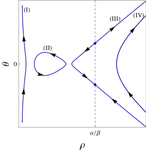
Figure 1: Identification of different branches for a closed Universe in $\rho$-$\theta$ parameter plane corresponding to different generic features of the solutions of equation (49) with and without a cosmological constant.

The branch (I) is a very well known result that exist even in the case where $\beta=0$. It describes a closed Universe with a cosmological constant.

However the branch (II) represents a cyclic Universe. Let us consider a collapse of a Universe where the initial density is considered in the branch (II). As it proceeds the density increases (see Fig.2) and reaches the maximum. This would then lead to defocusing and the collapse will end into a rebound ($\theta=0$) rather than a caustics. This is an effect due to the $R^{2}$ modification together with the cosmological constant. A necessary condition for the existence of the cyclic Universe is $0<\beta\Lambda<1/24$, which implies the extreme importance of the two constants (i.e. $\beta$ and $\Lambda$) in the existence of the cyclic Universe. After the rebound, the density decreases in an expanding Universe. At small densities, the model will have an other rebound which creates the cyclic Universe. This solution exist only for a closed Universe and has a maximum periodicity $T\propto 100\sqrt{\beta}$. However the variation of the density of matter for the same Universe would be $\Delta\rho\propto 0.5M_{Pl}^{2}/\beta$.

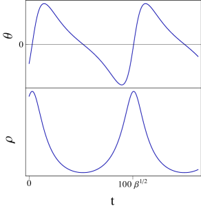
Figure 2: Evolution of $\theta$ and $\rho$ for the cyclic Universe corresponding to a periodic solution.

By considering $\beta\propto H_{0}^{-2}$, the Universe will have a periodicity larger that the Hubble time but at the same tine, the density of matter will have an extremely small variation $\Delta\rho/\rho_{0}\propto 1$ where $\rho_{0}$ is the density today.

VI Conclusion

One of the natural generalizations of the Riemannian nature of space-time is the Weyl space-time. Ehlers et al. Ehlers had already shown that the Weyl space-time is indeed the most general structure for the study of gravitational field as a geometric field. Such generalizations are quite pertinent in addressing the present day observational challenges posed in terms of the dark matter and the dark energy at one hand while the conceptual challenges posed by various black hole space-times and singularity in the theoretical front on the other. In the present work, we have developed a general framework for the Weyl space-time which reduces to the Weyl integral space-time (WIST) for the Starobinsky modification in $f(R)$ gravity in Einstein-Palatini formalism (EPF). In EPF, the Weyl field turns out to be an undetermined gauge and the space-time turns toWeylian from the Riemannian as soon as the matter is added to it.

The issue of caustics formation is very critical to the location of occurrence of singularity in certain region of space-time and we have performed a detailed analysis of this and have applied it, as a trivial example, to the $f(R)$ gravity cosmological models. It is found that the model $R+\beta R^{2}-2\Lambda$ clubbed with the Weyl field does indeed avoid the big-bang singularity which is already true without the $\beta-$correction. For the Starobinsky modified gravity along with the suitable initial conditions, it is possible to have a singularity free cyclic Universe which has unfortunately a very short periodicity. It is a pity that the model is not cosmologically viable, however it offers an interesting example of a non-singular cyclic model.

References

- (1) S. W. Hawking, G. F. R. Ellis, Cambridge University Press, Cambridge, 1973.
- (2) R. M. Wald, Chicago, USA: Chicago University Press ( 1984) 491p.
- (3) P. S. Joshi, Oxford, UK: Clarendon (1993) 377 p. (International series of monographs on physics, 87).
- (4) G. F. R. Ellis, Gen. Rel. Grav. 41 (2009) 581-660.
- (5) S. M. Carroll, gr-qc/9712019.
- (6) W. H. Kinney, arXiv:0902.1529 [astro-ph.CO]; D. Baumann, arXiv:0907.5424 [hep-th].
- (7) Y. Fujii and K. Maeda, Cambridge, USA: Cambridge University Press (2003) 240 p
- (8) A. Albrecht, P. J. Steinhardt, Phys. Rev. Lett. 48 (1982) 1220-1223.
-
(9)
Marzke, R. F. The Theory of Measurement in General Relativity. A.B. senior thesis,
Princeton (1959);
Kundt, W., and Hoffmann, B. Recent developments in General Relativity (Pergamon Press, New York, 1962);
Marzke, R. F., and Wheeler, J. A. Gravitation and relativity, (ed. H.Y. Chiu and W. F. Hoffman). New-York (1964). - (10) Ehlers, J.; Pirani, F.A.E.; Schild, A. The geometry of free fall and light propagation, in General Relativity, Papers in honour of J.L. Synge, Oxford: Clarendon Press (1972)
- (11) F. P. Poulis, J. M. Salim, arXiv:1106.3031 [gr-qc].
- (12) L. Fatibenea, M. Francaviglia, arXiv:1106.1961 [gr-qc].
- (13) E. Poisson, A Relativists Toolkit: The Mathematics of Black Hole Mechanics, Cambridge University Press, 2004.
- (14) A. Dasgupta, H. Nandan and S. Kar, Phys. Rev. D79 (2009) 124004.
- (15) G. Sardanashvily and V. Yanchevsky, Acta Physica Polonica B17 (1986) 1017.
- (16) G. N. Felder, Lev Kofman, and A. Starobinsky, J. High Energy Phys. 09 (2002) 026
- (17) U.D. Goswami, H.Nandan and M. Sami, Phys. Rev. D82 (2010) 103530
- (18) S. Kar and S. Sengupta, Pramana 69 (2007) 49.
- (19) N. Dadhich, Pramana 69 (2007) 23; N Dadhich, gr-qc/0511123.
- (20) A. Dasgupta, H. Nandan and S. Kar, Annals Phys. 323 (2008) 1621; A. Dasgupta, H. Nandan and S. Kar, Int. J. Geom. Meth. Mod. Phys. 6 (2009) 645, Erratum-ibid. 07 (2010) 517; S. Ghosh, A. Dasgupta and S. Kar, Phys. Rev. D83 (2011) 084001.
- (21) A. A. Starobinsky, Phys. Lett. B91 (1980) 99-102.
- (22) S. M. Carroll, V. Duvvuri, M. Trodden and M. S. Turner, Phys. Rev. D70 (2004) 043528 [arXiv:astro-ph/0306438].
- (23) E. A. Poberii, Gen. Rel. Grav. 26 (1994) 1011-1054.
- (24) J. A. Schouten, Ricci Calculus (2nd ed.; Berlin, 1954)
- (25) H. R. Brown and O. Pooley, arXiv:gr-qc/9908048.
- (26) M. Novello, L. A. R. Oliveira, J. M. Salim, E. Elbaz, Int. J. Mod. Phys. D1 (1992) 641-677.
- (27) T. Y. Moon, J. Lee and P. Oh, Mod. Phys. Lett. A 25 (2010) 3129 [arXiv:0912.0432 [gr-qc]].
- (28) M. Novello and S. E. P. Bergliaffa, Phys. Rept. 463 (2008) 127 [arXiv:0802.1634 [astro-ph]].
- (29) H. Weyl, Space Time Matter, Dover
- (30) W. Pauli, Theory of Relativity (Pergamon, London, 1958)
- (31) J. M. Salim and S. L. Sautu, Class. Quant. Grav. 13 (1996) 353.
- (32) S. Cotsakis, J. Miritzis and L. Querella, J. Math. Phys. 40 (1999) 3063 [arXiv:gr-qc/9712025].
- (33) T. P. Sotiriou, Class. Quant. Grav. 23 (2006) 1253 [arXiv:gr-qc/0512017].