Study of some rare decays of $B_{s}$ meson in the fourth generation model

Abstract

We study some rare decays of $B_{s}$ meson governed by the quark level transitions $b\to s$, in the fourth generation model popularly known as SM4. Recently it has been shown that SM4, which is a simple extension of the SM3, can successfully explain several anomalies observed in the CP violation parameters of $B$ and $B_{s}$ mesons. We find that in this model due to the additional contributions coming from the heavy $t^{\prime}$ quark in the loop, the branching ratios and other observables in rare $B_{s}$ decays deviate significantly from their SM values. Some of these modes are within the reach of LHCb experiment and search for such channels are strongly argued.

I Introduction

The spectacular performance of the two asymmetric $B$ factories Belle and Babar provided us an unique opportunity to understand the origin of CP violation in a very precise way. Although, the results from the $B$ factories do not provide us any clear evidence of new physics, but there are few cases observed in the last few years, which have 2-3 $\sigma$ deviations from their corresponding SM expectations hfag . For example, the difference between the direct CP asymmetry parameters between $B^{-}\to\pi^{0}K^{-}$ and $\bar{B}^{0}\to\pi^{+}K^{-}$, which is expected to be negligibly small in the SM, but found to be nearly $15\%$. The measurement of mixing-induced CP asymmetry in several $b\to s$ penguin decays is not found to be same as that of $B_{d}\to J/\psi K_{s}$. Recently, a very largish CP asymmetry has been observed by the CDF and D0 collaborations cdf ; d0 in the tagged analysis of $B_{s}\to J/\psi\phi$ with value $S_{\psi\phi}\in[0.24,1.36]$. Within the SM this asymmetry is expected to be vanishingly small, which basically comes from $B_{s}-\bar{B}_{s}$ mixing phase. It should be noted that all these deviations are associated with the flavour changing neutral current (FCNC) transitions $b\to s$. It is well known that the FCNC decays are forbidden at the tree level in the standard model (SM) and therefore play a very crucial role to look for the possible existence of new physics (NP).

In this paper we would like to study some rare decays of $B_{s}$ meson involving $b\to s$ transitions. The study of $B_{s}$ meson has attracted significant attention in recent times because huge number of $B_{s}$ mesons are expected to be produced in the currently running LHCb experiment, which opened up the possibility to study $B_{s}$ meson with high statistical precision. These studies will not only play a dominant role to corroborate the results of $B$ mesons but also look for possible hints of new physics. Here we will consider the decay channels $B_{s}\to\phi\pi$, $B_{s}\to\phi\gamma$, $B_{s}\to\gamma\gamma$ and $B_{s}\to\mu^{+}\mu^{-}\gamma$ which are highly suppressed in the SM. We intend to analyze these decay channels both in the SM and in the fourth quark generation model 4gen , usually known as SM4. SM4 is a simple extension of the standard model with three generations (SM3) with the additional up-type ($t^{\prime}$) and down-type ($d^{\prime}$) quarks. It has been shown in Ref. ref1 , that the addition of a fourth family of quarks with $m_{t^{\prime}}$ in the range (400-600) GeV provides a simple explanation for the several deviations, that have been observed involving CP asymmetries in the $B,~{}B_{s}$ decays. The implications of fourth generation in various $B$ decays are discussed in 4gnp ; 4gnp1 ; rm3a ; rm3 ; lenz . The experimental search for fourth generation quarks has also received significant attention recently due to the operation of Large Hadron Collider. The CMS collaboration put a lower bound on the mass of $t^{\prime}$ as $m_{t^{\prime}}\gtrsim 450\,$ GeV cms1 and exclude the $b^{\prime}$-quark mass in the region 255 GeV $<m_{b^{\prime}}<361$ GeV at $95\%$ C.L. cms2 .

The paper is organized as follows.In section II we discuss the non-leptonic decay process $B_{s}\to\phi\pi$. The radiative decays $B_{s}\to\phi\gamma$ and $B_{s}\to\gamma\gamma$ are discussed in Sections III and IV. The process $B_{s}\to\mu^{+}\mu^{-}\gamma$ is presented in Section V and Section VI contains the Conclusion.

II $B_{s}\to\phi\pi$ Process

In this section we will discuss the non-leptonic decay mode $B_{s}\to\phi\pi$ which receives dominant contribution from electroweak penguins $b\to sq\bar{q}$ ($q=u,d$), as the QCD penguins are OZI suppressed, and the color-suppressed tree contribution $b\to u\bar{u}s$ is doubly Cabibbo suppressed. Therefore, this process is expected to be highly suppressed in the SM and hence serves as a suitable place to search for new physics. This decay mode has been studied in the SM using QCD factorization approach cheng and in the model with non-universal $Z^{\prime}$ boson kim .

The relevant effective Hamiltonian describing this process is given by rg

$${\cal H}_{eff}^{SM}=\frac{G_{F}}{\sqrt{2}}\left[V_{ub}V_{us}^{*}\sum_{i=1,2}C_{i}(\mu)O_{i}-V_{tb}V_{ts}^{*}\sum_{i=3}^{10}C_{i}(\mu)O_{i}\right]\;,$$ (1)

where $C_{i}(\mu)$’s are the Wilson coefficients evaluated at the $b$-quark mass scale, $O_{1,2}$ are the tree level current-current operators, $O_{3-6}$ are the QCD and $O_{7-10}$ are the electroweak penguin operators.

Here we will use the QCD factorization approach to evaluate the hadronic matrix elements as discussed in qcdf . The matrix elements describing the $B_{s}\to\phi$ transition can be parameterized in terms of various form factors ball as

$$\langle\phi(p^{\prime},\epsilon)|\bar{s}\gamma_{\mu}(1 - \gamma_{5})b|B_{s}(p)\rangle=-i\epsilon_{\mu}^{*}(m_{B_{s}}+m_{\phi})A_{1}(q^{2})$$ (2)

$$+ i(p+p^{\prime})_{\mu}(\epsilon^{*}\cdot q)\frac{A_{2}(q^{2})}{m_{B_{s}}+m_{\phi}}+iq_{\mu}(\epsilon^{*}\cdot q)\frac{2m_{\phi}}{q^{2}}(A_{3}(q^{2})-A_{0}(q^{2}))$$

$$+ \epsilon_{\mu\nu\rho\sigma}\epsilon^{*\nu}p^{\rho}p^{\prime\sigma}\frac{2V(q^{2})}{m_{B_{s}}+m_{\phi}},$$

where $p$ and $p^{\prime}$ are the momenta of $B_{s}$ and $\phi$ mesons, $q=p-p^{\prime}$ is the momentum transfer, $A_{1-3}(q^{2})$ and $V(q^{2})$ are various form factors describing the transition process. Using the decay constant of $\pi^{0}$ meson as

$$\langle\pi^{0}(q)|\frac{\bar{u}\gamma^{\mu}\gamma_{5}u-\bar{d}\gamma^{\mu}\gamma_{5}d}{\sqrt{2}}|0\rangle=i\frac{f_{\pi}}{\sqrt{2}}q^{\mu}\;,$$ (3)

one can obtain the transition amplitude for the process

$${\cal A}(B_{s}\to\phi\pi)=\frac{G_{F}}{2}f_{\pi}(\epsilon^{*}\cdot q)2m_{\phi}A_{0}(q^{2})\left(V_{ub}V_{us}^{*}a_{2}-\frac{3}{2}V_{tb}V_{ts}^{*}(-a_{7}+a_{9})\right)$$ (4)

where $\lambda_{q}=V_{qb}V_{qs}^{*}$. The parameters $a_{i}$’s are related to the Wilson coefficients $C_{i}$’s and the corresponding expressions can be found in Ref. qcdf .

The corresponding decay width is given as

$$\Gamma(B_{s}\to\phi\pi)=\frac{|{\bf p}_{cm}|^{3}}{8\pi m_{\phi}^{2}}\left|\frac{{\cal A}(B_{s}\to\phi\pi)}{\epsilon^{*}\cdot q}\right|^{2}\;,$$ (5)

where ${\bf p}_{cm}$ is the center of mass momentum of the outgoing particles.

Now we discuss about the CP violating observables for this process. To obtain these observables, we can symbolically represent the amplitude (4) as

$${\cal A}(\bar{B}_{s}\to\phi\pi)=(\epsilon^{*}\cdot q)[\lambda_{u}A_{u}-\lambda_{t}A_{t}]=-\lambda_{t}A_{t}(\epsilon^{*}\cdot q)\Big{[}1-r~{}a~{}e^{-i(\pi+\beta_{s}+\gamma+\delta)}\Big{]},$$ (6)

where $a=|\lambda_{u}/\lambda_{t}|$, $-\gamma$ is the weak phase of $V_{ub}$, $(\pi+\beta_{s})$ is the weak phase of $\lambda_{t}$, $r=|A_{u}/A_{t}|$, and $\delta$ is the relative strong phases between $A_{t}$ and $A_{u}$. From the above amplitude, the direct and mixing induced CP asymmetry parameters can be obtained as

$$A_{\phi\pi} = \frac{2ra\sin\delta\sin(\beta_{s}+\gamma)}{1+(ra)^{2}+2ra\cos\delta\cos(\beta_{s}+\gamma)}$$

$$S_{\phi\pi} = -\frac{2ra\cos\delta\sin(\beta_{s}+\gamma)+(ra)^{2}\sin(2\beta_{s}+2\gamma)}{1+(ra)^{2}+2ra\cos\delta\cos(\beta_{s}+\gamma)}\;.$$ (7)

For numerical evaluation, we use the particles masses, lifetime of $B_{s}$ meson from pdg . For the CKM elements we use the Wolfenstein parametrization with the values of the parameters as $\lambda=0.2253\pm 0.0007$, $A=0.808_{-0.015}^{+0.022}$, $\bar{\rho}=0.132_{-0.014}^{+0.022}$, $\bar{\eta}=0.341\pm 0.013$. The parameters of QCD factorization approach and the value of the form factor used $A_{0}^{B_{s}\to\phi}=0.32\pm 0.01$ are taken from cheng .

With these inputs we obtain the branching ratio for this process as

$${\rm Br}(B_{s}\to\phi\pi)=(1.26\pm 0.32)\times 10^{-7}\;,$$ (8)

which is consistent with the prediction of cheng ; kim .

The CP violating observables are found to be

$$S_{\phi\pi}=-0.23\;,~{}~{}~{}~{}~{}~{}~{}A_{\phi\pi}=0.1\;.$$ (9)

Our predicted direct CP asymmetry is lower than the prediction of cheng . This difference arises mainly because the sub-leading power corrections to the color suppressed tree amplitude $a_{2}$ has been included in Ref. cheng , which introduces a large strong phase.

Now we will analyze this process in the fourth generation model. In the presence of a sequential fourth generation there will be additional contributions due to the $t^{\prime}$ quark in the loop diagrams. Furthermore, due to the additional fourth generation there will be mixing between the $b^{\prime}$ quark the three down-type quarks of the standard model and the resulting mixing matrix will become a $4\times 4$ matrix ($V_{CKM4})$ and the unitarity condition becomes $\lambda_{u}+\lambda_{c}+\lambda_{t}+\lambda_{t^{\prime}}=0$, where $\lambda_{q}=V_{qb}V_{qs}^{*}$. The parametrization of this unitary matrix requires six mixing angles and three phases. The existence of the two extra phases provides the possibility of extra source of CP violation hou . In the presence of fourth generation there will be additional contribution both to the $B_{s}\to\phi\pi$ decay amplitude as well as to the $B_{s}-\bar{B}_{s}$ mixing phenomenon. However, since the new physics contribution to $B_{s}-\bar{B}_{s}$ mixing amplitude due to fourth generation model has been discussed in Ref. rm3 , we will simply quote the results from there.

Now we will consider the additional contribution to the decay amplitude due to the fourth quark generation model. In this model the new contributions are due to the $t^{\prime}$ quark in the penguin loops. Thus, the modified Hamiltonian becomes

$${\cal H}_{eff}=\frac{G_{F}}{\sqrt{2}}\biggr{[}\lambda_{u}(C_{1}O_{1}+C_{2}O_{2})-\lambda_{t}\sum_{i=3}^{10}C_{i}O_{i}-\lambda_{t^{\prime}}\sum_{i=3}^{10}C_{i}^{\prime}O_{i}\biggr{]}\;,$$ (10)

where $C_{i}^{\prime}$’s are the effective Wilson coefficients due to $t^{\prime}$ quark in the loop. To find the new contribution due to the fourth generation effect, first we have to evaluate the new Wilson coefficients $C_{i}^{\prime}$. The values of these coefficients at the $M_{W}$ scale can be obtained from the corresponding contribution from $t$ quark by replacing the mass of $t$ quark by $t^{\prime}$ mass in the Inami Lim functions inami . These values can then be evolved to the $m_{b}$ scale using the renormalization group equation rg . Thus, the obtained values of $C^{\prime}_{i=7-10}(m_{b})$ for two representative set of values i.e., $m_{t^{\prime}}=400$ and 500 GeV are as presented in Table-I.

Table 1: Numerical values of the Wilson coefficients $C_{i}^{\prime}$ for $m_{t^{\prime}}=400$ and 500 GeV.

$t^{\prime}$ mass	$C_{7}^{\prime}$	$C_{8}^{\prime}$	$C_{9}^{\prime}$	$C_{10}^{\prime}$
$m_{t^{\prime}}$=400 GeV	$~{}4.453\times 10^{-3}$	$~{}2.115\times 10^{-3}$	$~{}-0.029~{}$	$0.006~{}$
$~{}m_{t^{\prime}}$=500 GeV	$~{}7.311\times 10^{-3}$	$~{}3.199\times 10^{-3}$	$~{}-0.041~{}$	$0.009~{}$

Thus, in the presence of fourth generation model, one can obtain the transition amplitude for $B_{s}\to\phi\pi$ process from Eq. (10), which can be symbolically represented as

$${\cal A}(\bar{B}_{s}\to\phi\pi) = (\epsilon^{*}\cdot q)(\lambda_{u}A_{u}-\lambda_{t}A_{t}-\lambda_{t^{\prime}}A_{t^{\prime}})$$ (11)

$$= -\lambda_{t}A_{t}(\epsilon^{*}\cdot q)\Big{[}1+r~{}ae^{i(\beta_{s}+\gamma-\delta)}+r^{\prime}~{}b~{}e^{i(\phi_{s}-\beta_{s}+\delta_{1})}\Big{]},$$

where $b=|\lambda_{t^{\prime}}/\lambda_{t}|$, $r^{\prime}=|A_{t^{\prime}}/A_{t}|$, and $\delta_{1}$ is the relative strong phases between $A_{t^{\prime}}$ and $A_{t}$. From the above amplitude, the CP averaged branching ratio, direct and mixing induced CP asymmetry parameters can be obtained as

$${\rm Br} = {\rm Br}^{\rm SM}~{}X\;,~{}~{}~{}~{}~{}~{}~{}~{}~{}~{}A_{\phi\pi}=\frac{Y}{X}\;,~{}~{}~{}~{}~{}~{}~{}~{}S_{\phi\pi}=-\frac{Z}{X},$$ (12)

with

$$X = 1+(ra)^{2}+(r^{\prime}b)^{2}+2ra\cos\delta\cos(\beta_{s}+\gamma)+2r^{\prime}b\cos\delta_{1}\cos(\phi_{s}-\beta_{s})$$

$$+ 2rr^{\prime}ab\cos(\phi_{s}+\gamma)\cos(\delta+\delta_{1})\;,$$

$$Y = 2ra\sin\delta\sin(\beta_{s}+\gamma)+2r^{\prime}b\sin\delta_{1}\sin(\phi_{s}-\beta_{s})+2rr^{\prime}ab\sin(\phi_{s}+\gamma)\sin(\delta+\delta_{1})\;,$$

$$Z = \sin 2\theta+2ra\cos\delta\sin(\beta_{s}+\gamma+2\theta)-2r^{\prime}b\cos\delta_{1}\sin(\phi_{s}-\beta_{s}-2\theta)$$ (13)

$$+ r^{2}a^{2}\sin(2\beta_{s}+2\gamma+2\theta)-r^{\prime 2}b^{2}\sin(2\phi_{s}-2\beta_{s}-2\theta)$$

$$- 2rr^{\prime}ab\cos(\delta+\delta_{1})\sin(\phi_{s}-2\beta_{s}-\gamma-2\theta).$$

In Eq. (13), $2\theta$ is the additional contribution to the $B_{s}-\bar{B}_{s}$ mixing phase in the fourth generation and the expression for it can be found in Ref. rm3 .

For numerical evaluation using the values of the new Wilson coefficients as presented in Table-I, we obtain $r\approx 7.79$, $\delta\approx 25.9^{\circ}$, $r^{\prime}=3.48$ (5.03), and $\delta_{1}\approx-0.1^{\circ}$ ($-0.1^{\circ}$) for $m_{t^{\prime}}=400$ (500) GeV. For the new CKM elements $\lambda_{t^{\prime}}$, we use the allowed range of $|\lambda_{t^{\prime}}|=(0.08-1.4)\times 10^{-2}$ [$(0.06-0.9)\times 10^{-2}$] and $\phi_{s}=(0\to 80)^{\circ}$ [$\phi_{s}=(0\to 80)^{\circ}$] for $m_{t^{\prime}}=400$ GeV [500 GeV], extracted using the available observables mediated through $b\to s$ transitions ref1 . Now varying $\lambda_{t}^{\prime}$ and $\phi_{s}$ in their allowed ranges, we show the variation of branching ratio in the left panel of Figure-1 and the correlation plot between the CP violating parameters in the right panel. From the figure it can be seen that the branching ratio is significantly enhanced from its SM value and large mixing-induced CP violation ($S_{\phi\pi}$) could be possible for this decay mode in the fourth generation model. However, the direct CP asymmetry does not deviate much from the corresponding SM value. It should also be noted that the branching ratio decreases slowly with the increase of $t^{\prime}$ mass. However, there is no significant $m_{t^{\prime}}$ dependence of the CP violating observables.

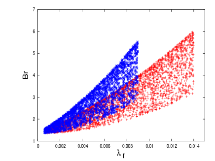
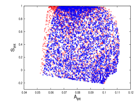
Figure 1: Variation of the CP averaged Branching ratio in units of $10^{-7}$ (left panel) and the Correlation plot between the mixing induced CP asymmetry $S_{\phi\pi}$ and the direct CP asymmetry parameter $A_{\phi\pi}$ (right panel) for the $B_{s}\to\phi\pi$ process. The red (blue) regions correspond to $m_{t^{\prime}}$=400 GeV (500 GeV)

III $B_{s}\to\phi\gamma$

Here we will consider the decay channel $B_{s}\to\phi\gamma$ which is induced by the quark level transition $\bar{b}\to\bar{s}\gamma$. This mode is the strange counterpart of the $B\to K^{*}\gamma$, which is very clean to analyze. Compared to $B_{d}$ meson the new elements of $B_{s}$ mesons are the small mixing phase $\phi_{s}$ and the large width difference $\Delta\Gamma_{s}$ of the $B_{s}$ meson. The branching ratio of this mode is recently reported by the Belle collaboration bel

$${\rm Br}(B_{s}\to\phi\gamma)=(57_{-15}^{+18}(\rm stat)_{-11}^{+12}(\rm syst))\times 10^{-6}\;.$$ (14)

In the standard model the CP averaged branching ratio of this mode is predicted to be ball1

$${\rm Br}(B_{s}\to\phi\gamma)=(39.4\pm 10.7\pm 5.3)\times 10^{-6}\;.$$ (15)

Although, the SM prediction seems to be consistent with the observed value, but the presence of large experimental uncertainties makes it difficult to infer/rule out the presence of new physics from this mode.

The transition process $b\to s\gamma$ can be described by the dipole type effective Hamiltonian which is given as buras

$${\cal H}_{eff}=-\frac{4G_{F}}{\sqrt{2}}\lambda_{t}C_{7}(m_{b})O_{7},$$ (16)

where $C_{7}$ is the Wilson coefficient and $O_{7}$ is the electromagnetic dipole operator given as

$$O_{7}=\frac{e}{32\pi^{2}}F_{\mu\nu}[m_{b}\bar{s}\sigma^{\mu\nu}(1+\gamma_{5})b+m_{s}\bar{s}\sigma^{\mu\nu}(1-\gamma_{5})b]$$ (17)

The expression for calculating the Wilson coefficient $C_{7}(\mu)$ is given in buras .

The matrix elements of the various hadronic currents between initial $B_{s}$ and the final $\phi$ meson, which are parameterized in terms of various form factors as ball

$$\langle\phi(p^{\prime},\epsilon|\bar{s}\sigma_{\mu\nu}q^{\nu}(1+\gamma_{5})b|B_{s}\rangle = i\epsilon_{\mu\nu\rho\sigma}\epsilon^{*\nu}p^{\rho}p^{\prime\sigma}2T_{1}(q^{2})$$ (18)

$$+ T_{2}(q^{2})[\epsilon_{\mu}^{*}(m_{B_{s}}^{2}-m_{\phi}^{2})-(\epsilon^{*}\cdot q)(p+p^{\prime})_{\mu}]\;,$$

with $T_{1}(0)=T_{2}(0)$ and $q=p-p^{\prime}$. With these definition of form factors, one can obtain the corresponding decay width as

$$\Gamma(B_{s}\to\phi\gamma)=\frac{\alpha G_{F}^{2}}{32\pi^{4}}|V_{tb}V_{ts}^{*}|^{2}|C_{7}^{eff}|^{2}m_{b}^{2}m_{B_{s}}^{3}|T_{1}(0)|^{2}\left(1-\frac{m_{\phi}^{2}}{m_{B_{s}}^{2}}\right)^{3}\;.$$ (19)

Using the value of the form factor $T_{1}(0)=0.349\pm 0.033$ ball , $C_{7}(m_{b})=-0.31$, and the values of the other parameters as discussed in section II, we obtain the branching ratio as

$${\rm Br}(B_{s}\to\phi\gamma)=(39.9\pm 12.3)\times 10^{-6}\;.$$ (20)

As is well known the rare radiative decays of $B$ mesons are particularly sensitive to the contributions from new physics. The $V-A$ structure of the weak interactions can be tested in FCNC decays of the type $b\to(s,d)\gamma$, since the emitted photon is predominantly left handed. The crucial point is that the leading operator $O_{7}\sim\bar{s}\sigma_{\mu\nu}F^{\mu\nu}b_{L(R)}$ necessitates a helicity flip on the external quark legs, which introduces a natural hierarchy between the left and right handed component of the order $m_{d,s}/m_{b}$. However it is difficult to measure the helicity of photon directly. It was pointed out long back that the time dependent CP asymmetry is an indirect measure of the photon helicity atwood , since it is caused by the interference of left and right handed helicity amplitudes. The final state in $B_{s}\to\phi\gamma$ is not a pure CP eigenstates. Rather in the SM they consist of equal mixture of positive and negative eigenvalues. Thus, due to an almost complete cancelation between positive and negative CP eigenstates, the asymmetries in $b\to s\gamma$ is very small. They are given by $m_{s}/m_{b}$ where the quark masses are current quark masses.

The normalized CP asymmetry for the $B_{s}\to\phi\gamma$ is defined as follows zwicky

$$A_{CP}(B_{s}\to\phi\gamma)=\frac{\Gamma(\bar{B}_{s}\to\phi_{s}\gamma)-\Gamma(B_{s}\to\phi\gamma)}{\Gamma(\bar{B}_{s}\to\phi_{s}\gamma)+\Gamma(B_{s}\to\phi\gamma)}\;,$$ (21)

where the left and right handed photon contributions are added incoherently i.e., $\Gamma(B_{s}\to\phi\gamma)=\Gamma(B_{s}\to\phi\gamma_{L})+\Gamma(B_{s}\to\phi\gamma_{R})$. It is well known that, the neutral mesons exhibit the time dependent CP asymmetry through mixing, i.e., if the particle and the antiparticle decay into a common final state $f$. In $B_{s}\to\phi\gamma$ this accounts to

$$B_{s}\rightarrow\phi\gamma_{L(R)}\leftarrow\bar{B}_{s}$$ (22)

With $|q/p|=1$, the CP asymmetry assumes the following generic time dependent form

$$A_{CP}(t)=\frac{S\sin(\Delta m_{s}t)-C\cos(\Delta m_{s}t)}{\cosh\frac{\Delta\Gamma_{s}t}{2}-H\sinh{\Delta\Gamma_{s}t}{2}}$$ (23)

In terms of the left and right handed amplitudes

$${\cal A}_{L(R)}={\cal A}(B_{s}\to\phi\gamma_{L(R)}),~{}~{}~{}~{}\bar{\cal A}_{L(R)}={\cal A}(\bar{B}_{s}\to\phi\gamma_{L(R)}),$$ (24)

the form of the observables $C$, $S$ and $H$ can be found as

$$C=\frac{(|{\cal A}_{L}|^{2}+|{\cal A}_{R}|^{2})-(|\bar{\cal A}_{L}|^{2}+|\bar{\cal A}_{R}|^{2})}{|{\cal A}_{L}|^{2}+|{\cal A}_{R}|^{2}+|\bar{\cal A}_{L}|^{2}+|\bar{\cal A}_{R}|^{2}}\;,$$

$$S=\frac{2{\rm Im}[\frac{q}{p}(\bar{\cal A}_{L}{\cal A}_{L}^{*}+\bar{\cal A}_{R}{\cal A}_{R}^{*})]}{|{\cal A}_{L}|^{2}+|{\cal A}_{R}|^{2}+|\bar{\cal A}_{L}|^{2}+|\bar{\cal A}_{R}|^{2}}\;,$$

$$H=\frac{2{\rm Re}[\frac{q}{p}(\bar{\cal A}_{L}{\cal A}_{L}^{*}+\bar{\cal A}_{R}{\cal A}_{R}^{*})]}{|{\cal A}_{L}|^{2}+|{\cal A}_{R}|^{2}+|\bar{\cal A}_{L}|^{2}+|\bar{\cal A}_{R}|^{2}}\;.$$ (25)

In the standard model the leading operator $O_{7}$, which allows the $\bar{B}_{s}(B_{s})$ meson to decay predominantly into a left (right) handed photon whereas $B_{s}(\bar{B}_{s})$ meson decaying into the left (right) handed photon suppressed by an $m_{s}/m_{b}$ chirality factor. Due to the interference between mixing and decay in $B_{s}\to\phi\gamma$, a single weak decay amplitude proportional to $\lambda_{t}$ is exactly canceled by the mixing phase and hence one can obtain $S_{\phi\gamma}=0$ and $H_{\phi\gamma}=2m_{s}/m_{b}$ zwicky .

The situation can be significantly modified in certain models beyond the standard model by new terms in the decay amplitudes and also by the new contribution to the $B_{s}-\bar{B}_{s}$ mixing. In this section we will study the effect of fourth quark generation on the various decay observables. In the presence of fourth generation, the Wilson coefficients $C_{7}$ will be modified due to the new contributions arising from the virtual $t^{\prime}$ quark in the loop. Thus, these modified coefficients can be represented as

$$C_{7}^{\rm tot}(\mu) = C_{7}(\mu)+\frac{\lambda_{t^{\prime}}}{\lambda_{t}}C_{7}^{\prime}(\mu).$$ (26)

The new coefficients $C_{7}^{\prime}$ can be calculated at the $M_{W}$ scale by replacing the $t$-quark mass by $m_{t^{\prime}}$ in the loop functions. These coefficients then to be evolved to the $b$ scale using the renormalization group equation as discussed in rg . The values of the new Wilson coefficients at the $m_{b}$ scale for $m_{t^{\prime}}=400$ GeV is given by $C_{7}^{\prime}(m_{b})=-0.375$.

Thus, including the new physics contribution due to fourth generation effect the branching ratio can be obtained from Eq. (19) by replacing $C_{7}$ by $C_{7}^{tot}$ and the CP violating parameters are given as

$$S_{\phi\gamma}=\frac{m_{s}}{m_{b}}\left(\frac{-C_{7}^{2}\sin 2\theta+2aC_{7}C_{7}^{\prime}\sin(\phi_{s}-\beta_{s}-2\theta)+a^{2}C_{7}^{\prime 2}\sin 2(\phi_{s}-\beta_{s}-\theta)}{C_{7}^{2}+r^{2}C_{7}^{\prime 2}+2aC_{7}C_{7}^{\prime}\cos(\phi_{s}-\beta_{s})}\right)\;,$$ (27)

$$H_{\phi\gamma}=\frac{m_{s}}{m_{b}}\left(\frac{C_{7}^{2}\cos 2\theta+a^{2}C_{7}^{\prime 2}\cos 2(\phi_{s}-\beta_{s}-\theta)+2aC_{7}C_{7}^{\prime}\cos(\phi_{s}-\beta_{s}-2\theta)}{C_{7}^{2}+a^{2}C_{7}^{\prime 2}+2aC_{7}C_{7}^{\prime}\cos(\phi_{s}-\beta_{s})}\right)\;,$$ (28)

where $2\theta$ is the new contribution to $B_{s}-\bar{B}_{s}$ mixing phase due to fourth generation. Now varying $\lambda_{t^{\prime}}$ between $(0.08-1.4)\times 10^{-2}$ and $\phi_{s}$ between $(0-80)^{\circ}$ we show in Figure-2, the CP averaged branching ratio (left panel) and the correlation plot between the CP violating observables (right panel). From the figure it can be seen that small but nonzero CP violating observables could be possible in the fourth generation model, while the branching ratio still consistent with the observed value. Furthermore, in this case also the branching ratio decreases with the increase of $t^{\prime}$-mass.

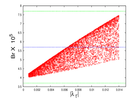
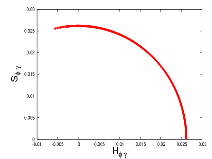
Figure 2: Variation of the CP averaged Branching ratio (left panel) and the Correlation plot between the CP violating observables $S_{\phi\gamma}$ and $H_{\phi\gamma}$ (right panel) for the $B_{s}\to\phi\gamma$ process. The horizontal blue line on the left panel is the central value of the measured branching ratio whereas the green lines represent the corresponding 1-sigma range.

IV $B_{s}\to\gamma\gamma$

Now we will discuss the decay process $B_{s}\to\gamma\gamma$. At the quark level this process is similar to $b\to s\gamma$. Up to the correction of order $1/M_{W}^{2}$, the effective Hamiltonian for $b\to s\gamma\gamma$ at scales $\mu_{b}=O(m_{b})$ is identical to the one for $b\to s\gamma$. The $B_{s}\to\gamma\gamma$ process has been studied extensively in the SM and in various new physics scenarios buc ; gam1 ; gam2 ; gam3 ; gam4 ; gam5 . The present experimental limit on the decay $B_{s}\to\gamma\gamma$ is bel

$$Br(B_{s}\to\gamma\gamma)\leq 8.7\times 10^{-6}~{}~{}~{}~{}(90\%~{}~{}C.L.).$$ (29)

We expect with the continuous accumulation of the experimental data, the situation will improve and the branching ratio will be more precise.

The effective Hamiltonian for this process is given by Eq. (16). To calculate the decay amplitude for this process one may follow the procedure discussed in Ref. gam3 . In order to calculate the matrix element of Eq. (16) for $B_{s}(p_{B})\to\gamma(k_{1})\gamma(k_{2})$, one can work in the weak binding approximation and assume that both the $b$ and $s$ quarks are at rest in the $B_{s}$ meson and the $b$ quark carries most of the meson energy and its four velocity can be treated as equal to that of $B_{s}$. Hence one may write $b$ quark momentum as $p_{b}=m_{b}v$, where $v$ is the common four velocity of $b$ and $B_{s}$. Thus we have

$$p_{b}\cdot k_{1}=m_{b}v\cdot k_{1}=\frac{1}{2}m_{b}m_{B_{s}}=p_{b}\cdot k_{2}$$

$$p_{s}\cdot k_{1}=(p-k_{1}-k_{2})\cdot k_{1}=-\frac{m_{B_{s}}}{2}(m_{B_{s}}-m_{b})=p_{s}\cdot k_{2}$$ (30)

The amplitude for $B_{s}\to\gamma\gamma$ can be computed using the following matrix elements

$$\langle 0|\bar{s}\gamma^{\mu}\gamma_{5}b|B_{s}(p_{B})\rangle=if_{B_{s}}{p_{B}}^{\mu}$$

$$\langle 0|\bar{s}\gamma_{5}b|B_{s}\rangle=if_{B_{s}}M_{B_{s}}$$ (31)

Thus, one can obtain the total amplitude for this process containing CP even and CP odd parts as

$${\cal A}(B_{s}\to\gamma\gamma)=M^{+}F_{\mu\nu}F^{\mu\nu}+iM^{-}F_{\mu\nu}\tilde{F}^{\mu\nu}\;,$$ (32)

with

$$M^{+}=-\frac{4\sqrt{2}\alpha G_{F}}{9\pi}f_{B_{s}}m_{B_{s}}V_{tb}V_{ts}^{*}\left(Bm_{b}K(m_{b}^{2})+\frac{3C_{7}}{8\bar{\Lambda}}\right)\;,$$ (33)

and

$$M^{-}=\frac{4\sqrt{2}\alpha G_{F}}{9\pi}f_{B_{s}}m_{B_{s}}V_{tb}V_{ts}^{*}\left(\sum_{q}m_{B_{s}}A_{q}J(m_{q}^{2})+m_{b}BL(m_{b}^{2})+\frac{3C_{7}}{8\bar{\Lambda}}\right)\;,$$ (34)

where $\bar{\Lambda}=m_{B_{s}}-m_{b}$. The parameters $A_{q}$’s are related to the Wilson coefficients $C_{i}$’s, which are evaluated at the $m_{b}$ scale as

$$A_{u} = (C_{3}-C_{5})N_{c}+(C_{4}-C_{6})$$

$$A_{d} = \frac{1}{4}[(C_{3}-C_{5})N_{c}+(C_{4}-C_{6})]$$

$$A_{c} = (C_{1}+C_{3}-C_{5})N_{c}+C_{2}+C_{4}-C_{6}$$

$$A_{s} = =A_{b}=\frac{1}{4}[(C_{3}+C_{4}-C_{5})N_{c}+(C_{3}+C_{4}-C_{6})]$$

$$B = C=-\frac{1}{4}(C_{6}N_{c}+C_{5})$$ (35)

The functions $J(m^{2})$, $K(m^{2})$ and $L(m^{2})$ are defined as

$$J(m^{2}) = I_{11}(m^{2})$$

$$K(m^{2}) = 4I_{11}(m^{2})-I_{00}(m^{2})$$

$$L(m^{2}) = I_{00}(m^{2})\;,$$ (36)

with

$$I_{pq}(m^{2})=\int_{0}^{1}dx\int_{0}^{1-x}dy\frac{x^{p}y^{q}}{m^{2}-2k_{1}\cdot k_{2}xy-i\epsilon}\;.$$ (37)

Thus, one can obtain the decay width of $B_{s}\to\gamma\gamma$ is

$$\Gamma(B_{s}\to\gamma\gamma)=\frac{m_{B_{s}}^{3}}{16\pi}\left(|M^{+}|^{2}+|M^{-}|^{2}\right)\;.$$ (38)

To obtain the numerical results we use the parameters as presented in section II. Thus, we obtain the branching ratio as

$${\rm Br}(B_{s}\to\gamma\gamma)=(1.8\pm 0.4)\times 10^{-7}\;,$$ (39)

which is lower than the present experimental upper bound bel .

In the sequential fourth generation model there exist additional contribution to $b\to s\gamma$ induced by the 4th generation up type quarks $t^{\prime}$. The new Wilson coefficients can be obtained from those of their $t$ counter parts by replacing the mass of $t$ quark by $t^{\prime}$ at the $M_{W}$ scale, which is then evolved to the $m_{b}$ scale using the renormalization group approach. As discussed in the previous section the values of the new Wilson coefficients at the $m_{b}$ scale for $m_{t^{\prime}}=400$ GeV is given by $C_{7}^{\prime}(m_{b})=-0.375$. At the scale $m_{b}$, the modified Wilson coefficient of the dipole operator becomes

$$C_{7}^{\rm tot}(m_{b})=C_{7}(m_{b})+\frac{V_{t^{\prime}b}V_{t^{\prime}s}^{*}}{V_{tb}V_{ts}^{*}}C_{7}^{\prime}(m_{b})\;.$$ (40)

Now varying $\lambda_{t^{\prime}}$ between $(0.08-1.4)\times 10^{-2}$ and $\phi_{s}$ between $(0-80)^{\circ}$ we show in Figure-3, the branching ratio for $B_{s}\to\gamma\gamma$ process.From the figure it can be the branching ratio can be enhanced from its SM value, but the enhancement is not so significant.

Figure 3: Variation of the Branching ratio for the process $B_{s}\to\gamma\gamma$ process.

V $B_{s}^{0}\to\mu^{+}\mu^{-}\gamma$ process

Now let us consider the radiative di-leptonic decay modes $B_{s}\to\mu^{+}\mu^{-}\gamma$, which are also very sensitive to the existence of new physics beyond the SM. Due to the presence of the photon in the final state, this decay mode is free from helicity suppression, but it is further suppressed by a factor of $\alpha$ with respect to the pure leptonic $B_{s}\to\mu^{+}\mu^{-}$ process. However, in spite of this $\alpha$ suppression, the radiative leptonic decay $B_{s}\to\mu^{+}\mu^{-}\gamma$, has comparable decay rate as that of purely leptonic ones.

The effective Hamiltonian describing this process $B_{s}\to\mu^{+}\mu^{-}$ is rg

$${\cal{H}}_{eff} = \frac{G_{F}\alpha}{\sqrt{2}\pi}V_{tb}V_{ts}^{*}\Bigg{[}C^{eff}_{9}~{}({\bar{s}}~{}\gamma_{\mu}~{}P_{L}~{}b)({\bar{l}}~{}\gamma^{\mu}~{}l)+C_{10}~{}({\bar{s}}~{}\gamma_{\mu}~{}P_{L}~{}b)({\bar{l}}~{}\gamma^{\mu}~{}\gamma_{5}~{}l)$$ (41)

$$~{}~{}~{}~{}~{}~{}~{}-\frac{2C_{7}~{}m_{b}}{q^{2}}({\bar{s}}i\sigma_{\mu\nu}q^{\nu}P_{R}~{}b)({\bar{l}}~{}\gamma^{\mu}~{}l)\Bigg{]}\;,$$

where $l$ is the short hand notation for $\mu$, $P_{L,R}=\frac{1}{2}~{}(1\mp\gamma_{5})$ and $q$ is the momentum transfer. $C_{i}$’s are the Wilson coefficients evaluated at the $b$ quark mass scale in NLL order with values beneke

$$C_{7}^{eff}=-0.31\;,~{}~{}C_{9}=4.154\;,~{}~{}C_{10}=-4.261\;.$$ (42)

The coefficient $C_{9}^{eff}$ has a perturbative part and a resonance part which comes from the long distance effects due to the conversion of the real $c\bar{c}$ into the lepton pair $l^{+}l^{-}$. Hence, $C_{9}^{eff}$ can be written as

$$C_{9}^{eff}=C_{9}+Y(s)+C_{9}^{res}\;,$$ (43)

where the function $Y(s)$ denotes the perturbative part coming from one loop matrix elements of the four quark operators and is given in Ref. buras . The long distance resonance effect is given as res

$$C_{9}^{res}=\frac{3\pi}{\alpha^{2}}(3C_{1}+C_{2}+3C_{3}+C_{4}+3C_{5}+C_{6})\sum_{J/\psi,\psi^{\prime}}\kappa\frac{m_{V_{i}}\Gamma(V_{i}\to l^{+}l^{-})}{m_{V_{i}}^{2}-s-im_{V_{i}}\Gamma_{V_{i}}}\;,$$ (44)

where the phenomenological parameter $\kappa$ is taken to be 2.3, so as to reproduce the correct branching ratio ${\cal B}(B\to J/\psi K^{*}\to K^{*}l^{+}l^{-})={\cal B}(B\to J/\psi K^{*}){\cal B}(J/\psi\to l^{+}l^{-})$. In this analysis, we will consider only the contributions arising from two dominant resonances i.e., $J/\psi$ and $\psi^{\prime}$.

The matrix element for the decay $B_{s}\to\mu^{+}\mu^{-}\gamma$ can be obtained from that of the $B_{s}\to\mu^{+}\mu^{-}$ one by attaching the photon line to any of the charged external fermion lines. In order to calculate the amplitude, when the photon is radiated from the initial fermions (structure dependent (SD) part), we need to evaluate the matrix elements of the quark currents present in (41) between the emitted photon and the initial $B_{s}$ meson. These matrix elements can be obtained by considering the transition of a $B_{s}$ meson to a virtual photon with momentum $k$. In this case the form factors depend on two variables, i.e., $k^{2}$ (the photon virtuality) and the square of momentum transfer $q^{2}=(p_{B}-k)^{2}$. By imposing gauge invariance, one can obtain several relations among the form factors at $k^{2}=0$. These relations can be used to reduce the number of independent form factors for the transition of the $B_{s}$ meson to a real photon. Thus, the matrix elements for $B_{s}\to\gamma$ transition, induced by vector, axial-vector, tensor and pseudo-tensor currents can be parameterized as kruger

$$\langle\gamma(k,\varepsilon)|\bar{s}\gamma_{\mu}\gamma_{5}b|B_{s}(p_{B})\rangle = ie\left[\varepsilon_{\mu}^{*}(p_{B}\cdot k)-(\varepsilon^{*}\cdot p_{B})k_{\mu}\right]\frac{F_{A}}{m_{B_{s}}}\;,$$

$$\langle\gamma(k,\varepsilon)|\bar{s}\gamma_{\mu}b|B_{s}(p_{B})\rangle = e\epsilon_{\mu\nu\alpha\beta}\varepsilon^{*\nu}p_{B}^{\alpha}~{}k^{\beta}\frac{F_{V}}{m_{B_{s}}}\;,$$

$$\langle\gamma(k,\varepsilon)|\bar{s}\sigma_{\mu\nu}q^{\nu}\gamma_{5}b|B_{s}(p_{B})\rangle = e\left[\varepsilon_{\mu}^{*}(p_{B}\cdot k)-(\varepsilon^{*}\cdot p_{B})k_{\mu}\right]F_{TA}\;,$$

$$\langle\gamma(k,\varepsilon)|\bar{s}\sigma_{\mu\nu}q^{\nu}b|B_{s}(p_{B})\rangle = e\epsilon_{\mu\nu\alpha\beta}\varepsilon^{*\nu}p_{B}^{\alpha}~{}k^{\beta}F_{TV}\;,$$ (45)

where $\varepsilon$ and $k$ are the polarization vector and the four-momentum of photon, $p_{B}$ is the momentum of initial $B_{s}$ meson and $F_{i}$’s are the various form factors.

Thus, the matrix element describing the SD part takes the form

$${\cal M}_{SD} = \frac{\alpha^{3/2}G_{F}}{\sqrt{2\pi}}~{}V_{tb}V_{ts}^{*}\biggr{\{}\epsilon_{\mu\nu\alpha\beta}\varepsilon^{*\nu}p_{B}^{\alpha}~{}k^{\beta}\Big{(}A_{1}~{}\bar{l}\gamma^{\mu}l+A_{2}~{}\bar{l}\gamma^{\mu}\gamma_{5}l\Big{)}$$ (46)

$$+ i\Big{(}\varepsilon_{\mu}^{*}(k\cdot p_{B})-(\varepsilon^{*}\cdot p_{B})k_{\mu}\Big{)}\Big{(}B_{1}~{}\bar{l}\gamma^{\mu}l+B_{2}~{}\bar{l}\gamma^{\mu}\gamma_{5}l\Big{)}\biggr{\}}\;,$$

where

$$A_{1} = 2C_{7}\frac{m_{b}}{q^{2}}F_{TV}+C_{9}\frac{F_{V}}{m_{B_{s}}}\;,~{}~{}~{}~{}~{}~{}~{}~{}~{}~{}~{}~{}~{}A_{2}=C_{10}\frac{F_{V}}{m_{B_{s}}}\;,$$

$$B_{1} = -2C_{7}\frac{m_{b}}{q^{2}}F_{TA}-C_{9}\frac{F_{A}}{m_{B_{s}}}\;,~{}~{}~{}~{}~{}~{}~{}~{}~{}~{}~{}~{}B_{2}=-C_{10}\frac{F_{A}}{m_{B_{s}}}\;.$$ (47)

The form factors $F_{V}$ and $F_{A}$ have been calculated within the dispersion approach new1 . The $q^{2}$ dependence of the form factors are given as kruger

$$F(E_{\gamma})=\beta\frac{f_{B_{s}}m_{B_{s}}}{\Delta+E_{\gamma}}\;,$$ (48)

where $E_{\gamma}$ is the photon energy, which is related to the momentum transfer $q^{2}$ as

$$E_{\gamma}=\frac{m_{B_{s}}}{2}\left(1-\frac{q^{2}}{m_{B_{s}}^{2}}\right)\;.$$ (49)

The values of the parameters $\beta$ and $\Delta$ are given in Table-2. The same ansatz (48) has also been assumed for the form factors $F_{TA}$ and $F_{TV}$. We use the decay constant of the $B_{s}$ meson, which is evaluated in lattice QCD calculation as $f_{B_{s}}=232\pm 10$ MeV fbs .

Table 2: The parameters for $B_{s}\to\gamma$ form factors.

Parameter		$F_{V}$		$F_{TV}$		$F_{A}$		$F_{TA}$
$\beta({\rm GeV}^{-1})$		0.28		0.30		0.26		0.33
$\Delta({\rm GeV})$		0.04		0.04		0.30		0.30

When the photon is radiated from the outgoing lepton pairs, the internal bremsstrahlung (IB) part, the matrix element is given as

$${\cal M}_{IB}=\frac{\alpha^{3/2}G_{F}}{\sqrt{2\pi}}~{}V_{tb}V_{ts}^{*}~{}f_{B_{s}}~{}m_{\mu}~{}C_{10}\biggr{[}\bar{l}\left(\frac{\not\!{\varepsilon}^{*}{\not\!{p}}_{B}}{p_{+}\cdot k}-\frac{{\not\!{p}}_{B}\not\!{\varepsilon}^{*}}{p_{-}\cdot k}\right)\gamma_{5}~{}l\biggr{]}\;,$$ (50)

where $p_{+}$ and $p_{-}$ are the momenta of emitted $\mu^{+}$ and $\mu^{-}$ respectively. Thus, the total matrix element for the $B_{s}\to l^{+}l^{-}\gamma$ process is given as

$${\cal M}={\cal M}_{SD}+{\cal M}_{IB}\;.$$ (51)

The differential decay width of the $B_{s}\to\mu^{+}\mu^{-}\gamma$ process, in the rest frame of $B_{s}$ meson is given as

$$\frac{d\Gamma}{ds}=\frac{G_{F}^{2}\alpha^{3}}{2^{10}\pi^{4}}~{}|V_{tb}V_{ts}^{*}|^{2}~{}m_{B_{s}}^{3}~{}\Delta_{1}\;,$$ (52)

where

$$\Delta_{1} = \frac{4}{3}m_{B_{s}}^{2}(1-\hat{s})^{2}v_{l}\Big{(}(\hat{s}+2r_{l})(|A_{1}|^{2}+|B_{1}|^{2})+(\hat{s}-4r_{l})(|A_{2}|^{2}+|B_{2}|^{2}\Big{)}$$ (53)

$$- 64~{}\frac{f_{B_{s}}^{2}}{m_{B_{s}}^{2}}\frac{r_{l}}{1-\hat{s}}~{}C_{10}^{2}~{}\Big{(}(4r_{l}-\hat{s}^{2}-1)\ln\frac{1+v_{l}}{1-v_{l}}+2\hat{s}~{}v_{l}\Big{)}$$

$$- 32~{}r_{l}(1-\hat{s})^{2}~{}f_{B_{s}}{\rm Re}\Big{(}C_{10}A_{1}^{*}\Big{)},$$

with $s=q^{2}$, $\hat{s}=s/m_{B_{s}}^{2}$, $r_{l}=m_{\mu}^{2}/m_{B_{s}}^{2}$, $v_{l}=\sqrt{1-4m_{\mu}^{2}/q^{2}}$. The physical region of $s$ is $4m_{\mu}^{2}\leq s\leq m_{B_{s}}^{2}$.

The forward backward asymmetry is given as

$$A_{FB} = \frac{1}{\Delta_{1}}\biggr{[}2m_{B_{s}}^{2}\hat{s}(1-\hat{s})^{3}v_{l}^{2}~{}{\rm Re}\Big{(}A_{1}^{*}B_{2}+B_{1}^{*}A_{2}\Big{)}$$ (54)

$$+ 32~{}f_{B_{s}}~{}r_{l}(1-\hat{s})^{2}\ln\left(\frac{4r_{l}}{\hat{s}}\right){\rm Re}\Big{(}C_{10}B_{2}^{*}\Big{)}\biggr{]}\;.$$

We have shown the variation of the differential decay distribution (52) (in units of $10^{-7}$, and the forward backward asymmetry (54) for $B_{s}\to\mu^{+}\mu^{-}\gamma$ in Figure-4.

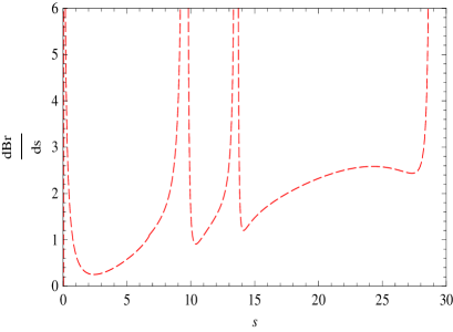
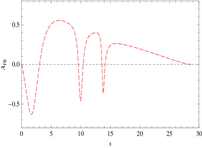
Figure 4: Variation of the differential branching ratio (in units of $10^{-10}$) (left panel) and the forward-backward asymmetry with respect to the momentum transfer $s$ (right panel) for the $B_{s}\to\mu^{+}\mu^{-}\gamma$ process.

As discussed earlier in the presence of fourth generation, the Wilson coefficients $C_{7,9,10}$ will be modified due to the new contributions arising from the virtual $t^{\prime}$ quark in the loop. Thus, these coefficients will be modified as

$$C_{7}^{\rm tot}(\mu) = C_{7}(\mu)+\frac{\lambda_{t^{\prime}}}{\lambda_{t}}C_{7}^{\prime}(\mu),$$

$$C_{9}^{\rm tot}(\mu) = C_{9}(\mu)+\frac{\lambda_{t^{\prime}}}{\lambda_{t}}C_{9}^{\prime}(\mu),$$

$$C_{10}^{\rm tot}(\mu) = C_{10}(\mu)+\frac{\lambda_{t^{\prime}}}{\lambda_{t}}C_{10}^{\prime}(\mu).$$ (55)

The new coefficients $C_{7,9,10}^{\prime}$ can be calculated at the $M_{W}$ scale by replacing the $t$-quark mass by $m_{t}^{\prime}$ in the loop functions as discussed in buras . These coefficients then to be evolved to the $b$ scale using the the renormalization group equation. The values of the new Wilson coefficients at the $m_{b}$ scale for $m_{t^{\prime}}=400$ GeV is given by $C_{7}^{\prime}(m_{b})=-0.375$, $C_{9}^{\prime}(m_{b})=5.831$ and $C_{10}^{\prime}=-17.358$.

Thus, one can obtain the differential branching ratio and the forward backward asymmetry in SM4 by replacing $C_{7,9,10}$ in Eqs (52) and (54) by $C_{7,9,10}^{\rm tot}$. Using the values of the $\lambda_{t^{\prime}}$ and $\phi_{s}$ for $m_{t^{\prime}}=400$ GeV as discussed earlier, the differential branching ratio and the forward backward asymmetry for $B_{s}\to\mu^{+}\mu^{-}\gamma$ is presented in Figure-5, where we have not considered the contributions from intermediate charmonium resonances. From the figure it can be seen that the differential branching ratio of this mode is significantly enhanced from its corresponding SM value whereas the forward backward asymmetry is slightly reduced with respect to its SM value. However, the zero-position of the FB asymmetry remains unchanged the fourth quark generation model.

To obtain the branching ratios it is necessary to eliminate the background due to the resonances $J/\psi(\psi^{\prime})$ with $J/\psi(\psi^{\prime})\to\mu^{+}\mu^{-}$. We use the following veto windows to eliminate these backgrounds

$$m_{J/\psi}-0.02<m_{\mu^{+}\mu^{-}}<m_{J/\psi}+0.02;$$

$$m_{\psi^{\prime}}-0.02<m_{\mu^{+}\mu^{-}}<m_{\psi^{\prime}}+0.02.$$

Furthermore, it should be noted that the $|{\cal M}_{IB}|^{2}$ has infrared singularity due to the emission of soft photon. Therefore, to obtain the branching ratio, we impose a cut on the photon energy, which will correspond to the experimental cut imposed on the minimum energy for the detectable photon. Requiring the photon energy to be larger than 25 MeV, i.e., $E_{\gamma}\geq\delta~{}m_{B_{s}}/2$, which corresponds to $s\leq m_{B_{s}}^{2}(1-\delta)$, and therefore, we set the cut $\delta\geq 0.01$. Thus, with the above defined veto windows and the infrared cutoff parameter, the total branching ratio for $B_{s}\to\mu^{+}\mu^{-}\gamma$ process is found to be

$${\rm Br}(B_{s}\to\mu^{+}\mu^{-}\gamma) = 5.6\times 10^{-9}\;,~{}~{}~{}~{}~{}~{}{(\rm SM)}$$ (56)

$$< 2.2\times 10^{-8}\;,~{}~{}~{}~{}~{}~{}~{}{\rm(for~{}m_{t^{\prime}}=400~{}GeV)}\;.$$

The above branching ratio is comparable with that of the corresponding pure-leptonic process, $B_{s}\to\mu^{+}\mu^{-}$, whose predicted branching ratio ref1 for $m_{t^{\prime}}=400$ GeV is

$${\rm Br}(B_{s}\to\mu^{+}\mu^{-}) < 0.8\times 10^{-8}\;.$$ (57)

The LHCb lcb has searched for this process and set the upper limit as ${\rm Br}(B_{s}\to\mu^{+}\mu^{-})<1.2~{}(1.5)\times 10^{-8}$ at $90\%$ ($95\%$) CL. Therefore, the $B_{s}\to\mu^{+}\mu^{-}\gamma$ decay channel could also be accessible there and hopefully it will be observed soon.

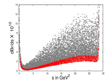
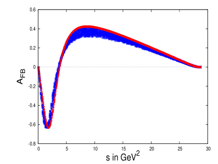
Figure 5: Variation of the differential branching ratio (left panel) and the forward-backward asymmetry with respect to the momentum transfer $s$ (right panel) for the $B_{s}\to\mu^{+}\mu^{-}\gamma$ process, in fourth quark generation model (red regions) whereas the corresponding SM values are shown in blue regions.

VI Conclusion

In this paper we have studied some rare decays of the $B_{s}$ meson in the fourth quark generation model. The large production of $B_{s}$ mesons at the LHC opens up the possibility to study $B_{s}$ meson with high statistical precision. The decay modes considered here are $B_{s}\to\phi\pi$, $B_{s}\to\phi\gamma$, $B_{s}\to\gamma\gamma$ and $B_{s}\to\mu^{+}\mu^{-}\gamma$, which are highly suppressed in the SM as they occurred only through one-loop diagrams. Therefore, they provide an ideal testing ground to look for new physics. The fourth generation model is a very simple extension of the SM with three generations and it can easily accommodate the observed anomalies in the $B$ and $B_{s}$ CP violation parameters for $m_{t^{\prime}}$ in the range of (400-600) GeV. We found that in the fourth generation model the branching ratios for these processes enhanced from their corresponding SM values. However, the mixing-induced CP asymmetry of in $B_{s}\to\phi\pi$ process enhanced significantly from its SM value. The CP violating observables in $B_{s}\to\phi\gamma$ are found to be small but nonzero. Some of these branching ratios are within the reach of LHCb experiments, hence the observation of these modes will provide us an indirect evidence for the existence of fourth quark generation.

Acknowledgments

RM would like to thank Council of Scientific and Industrial Research, Government of India, for financial support through Grant No. 03(1190)-11/EMR-II.

References

(1) Heavy Flavor Averaging Group, http://www.slac.stanford.edu/xorg/hfag.
(2) T. Aaltonen et al. [CDF Collaboration], Phys. Rev. Lett. 100,
161802 (2008), arXiv: 0712.2397 [hep-ex].
(3) V. M. Abazov et al. [D0 Collaboration], Phys. Rev. Lett.
101, 241801 (2008), arXiv:0802.2255 [hep-ex],
V. M. Abazov et al. [D0 Collaboration], Phys. Rev. Lett.
102, 032001 (2009), arXiv:0812.0037 [hep-ex].
(4) W. -S. Hou, A. Soni and H. Steger, Phys. Lett. B 192, 441 (1987); W. S. Hou, R. S. Willey and A. Soni, Phys. Rev.
Lett. 58, 1608 (1987).
(5) A. Soni, A. Alok, A. Giri, R. Mohanta and S.Nandi,
Phys. Lett. B 683, 302 (2010), arXiv:0807.1971 [hep-ph]; Phys.
Rev. D. 82, 033009 (2010), arXiv:1002.0595 [hep-ph].
(6) A. J. Buras et al, JHEP 1009, 106 (2010)
arXiv:1002.2126 [hep-ph].
(7) W. S. Hou and C. Y. Ma, Phys. Rev. D 82, 036002 (2010),
arXiv:1004.2186 [hep-ph].
(8) R. Mohanta and A. Giri, Phys. Rev. D 82, 094022 (2010),
arXiv:1010.1152 [hep-ph].
(9) R. Mohanta, Phys. Rev. D 84, 014019 (2011), arXiv:1104.4739 [hep-ph].
(10) O.Eberhardt, A. Lenz and J. Rohrwild, Phys. Rev. D. 82, 095006 (2010),
arXiv: 1005.3505 [hep-ph].
(11) CMS Collaboration, Search for a heavy top-like quark pairs at CMS in pp
collisions, (CMS-PAS-EXO-11-005), (2011);
CMS Collaboration, Search for pair production in lepton+jets channel, (CMS-PAS-EXO-11-051), (2011).
(12) S. Chatrchyan et al. [CMS Collaboration], Phys. Lett. B 701, 204 (2011),
aiXiv:1102.4746 [hep-ex].
(13) H.-Y. Cheng and C.-K. Chua, Phys.
Rev. D 80, 114026 (2009).
(14) J. Hua, C. S. Kim and Y. Li, arXiv:1002.2532 [hep-ph].
(15) G. Buchalla, A.J. Buras, M. Lautenbacher, Rev. Mod. Phys. 68, 1125 (1996).
(16) M. Beneke, G. Buchalla, M. Neubert and C.T. Sachrajda,
Nucl. Phys. B 606, 245 (2001); M. Beneke and M. Neubert,
Nucl.Phys. B 675, 333 (2003).
(17) P. Ball and R. Zwicky, Phys. Rev. D 71, 014029 (2005).
(18) K. Nakamura et al, Particle Data Group,
J. Physics G 37, 075021 (2010).
(19) W. S. Hou, Chin. J. Phs. 47, 134 (2009), arXiv:0803.1234 [hep-ph].
(20) T. Inami and C. S. Lim, Prog. Theor. Phys. 65,
297 (1981); ibid65, 1772 (1981).
(21) J. Wicht et al., Phys. Rev. Lett. 100, 121801 (2008),
arXiv:0712.2659 [hep-ex].
(22) P. Ball, G. W. Jones and R. Zwicky, Phys. Rev. D. 75,
054004 (2007).
(23) A. J. Buras and M. Munz, Phys. Rev. D 52, 186 (1995).
(24) D. Atwood, M. Gronau and A. Soni, Phys. Rev. Lett.
79, 185 (1997).
(25) F. Muheim, Y. Xie and R. Zwicky, Phys. Lett. B
664, 174 (2008).
(26) S. W. Bosch and G. Buchalla, JHEP 0208, 054 (2002).
(27) W. Huo, C. D. Lu and Z. Xiao, arXiv:hep-ph/0302177.
(28) G. Hiller and E. O. Iltan, Phys. Lett. B 409, 425 (1997).
(29) C. H. V. Chang, G. L. Lin and Y. P. Yao, Phys. Lett. B. 415, 395 (1997).
(30) T. M. Aliev and E.O. Iltan, Phys. Rev. D 58, 095014 (1998).
(31) H. Chen and W. Huo, arXiv: 1101.4660 [hep-ph].
(32) M. Beneke, Th. Fledmann and D. Seidel, Nucl. Phys.
B 612, 25 (2001).
(33) C. S. Lim, T. Morozumi and A. I. Sanda, Phys. Lett. B.
218, 343 (1989); N. G. Deshpande, J. Trampetic and K. Panose, Phys.
Rev. D 39, 1461 (1989);
P. J. O’Donnell and H. K.K. Tung, Phys. Rev. D 43, 2067 (1991);
P. J. O’Donnell, M. Sutherland and H. K.K. Tung, Phys. Rev. D 46,
4091 (1992).
(34) F. Krüger and D. Melikhov, Phys. Rev. D 67, 034002
(2003).
(35) M. Beyer, D. Melikhov, N. Nikitin and B. Stech,
Phys. Rev. D 64, 094006 (2001).
(36) P. Dimopoulos et al., [ETM Collaboration],
arxiv:1107.1441 [hep-lat].