Brownian motion Nonequilibrium and irreversible thermodynamics Molecular dynamics methods Fluctuation phenomena, random processes, noise, and Brownian motion

Generalised Einstein Relation for Hot Brownian Motion

Abstract

The Brownian motion of a hot nanoparticle is described by an effective Markov theory based on fluctuating hydrodynamics. Its predictions are scrutinized over a wide temperature range using large-scale molecular dynamics simulations of a hot nanoparticle in a Lennard-Jones fluid. The particle positions and momenta are found to be Boltzmann distributed according to distinct effective temperatures $T_{\mathrm{HBM}}$ and $T_{\mathrm{k}}$. For $T_{\mathrm{HBM}}$ we derive a formally exact theoretical prediction and establish a generalised Einstein relation that links it to directly measurable quantities.

Hot Brownian motion is the Brownian motion of nanoscopic colloidal particles that have an elevated temperature compared to their solvent[1]. The phenomenon is ubiquitous in modern biophysical and nanotechnological work, where one often relies on nanoparticles exposed to laser light as tracers, anchors, or self-propelling nanomachines[2, 3, 4, 5, 6, 7, 8]. In a number of innovative applications the heating of the particle is moreover deliberately exploited for detection, manipulation and surgery on the nanoscale [9, 10, 11, 12, 13]. In general, heat and vorticity diffuse much faster than the colloidal particles, typical diffusivities being on the order of $10^{-7}\,\mathrm{m}^{2}\,\mathrm{s}^{-1}$ versus $10^{-11}\ldots 10^{-10}\,\mathrm{m}^{2}\,\mathrm{s}^{-1}$, respectively. On the basis of this characteristic Brownian scale separation, one may treat the solvent temperature and velocity distributions as stationary radial fields $T(r)$, $\mathbf{u}(\mathbf{r})$ around the instantaneous particle position. To a good approximation, the hot Brownian motion of a single particle can thus be characterised as a stationary nonequilibrium process. It is then natural to seek an effective equilibrium description in terms of Markovian stochastic equations of motion with effective friction and temperature parameters [1, 14].

Such effective parameters are certainly valuable elements of any quantitative description or application, but it is also clear that they will be less universal and more context-sensitive than their conventional equilibrium counterparts. For example, one has to expect different effective parameters for different degrees of freedom of the colloidal particle, such as translational and rotational motion, and they differ not merely by simple geometric or kinematic factors [15]. Also momentum and conformational degrees of freedom turn out to be governed by distinct effective temperature, as already independently pointed out by Barrat and coworkers[16]. The best one can hope for is thus a systematic and quantitative understanding of the origin of the effective temperatures and transport coefficients pertaining to the observables most relevant in practice. This hope is justified by the observation that Brownian motion is a mesoscopic phenomenon and as such allows some coarse-graining over microscopic degrees of freedom. In other words, the effective temperatures and transport coefficients of the colloidal particle should emerge form the “middle world”[17] of stochastic thermodynamics[18] and fluctuating hydrodynamics[19, 20, 21] rather than directly from a much more intricate microscopic description. As a consequence, the effective parameters may still be expected to be reasonably insensitive to many of the usually elusive (and often accidental) microscopic details, such as the precise functional form of the atomic interactions.

While this is true in principle, the appropriate mesoscopic approach is not always entirely obvious and straightforward, a priori. Therefore, it is valuable to have direct access to a comprehensive microscopic characterisation of some model system. A standard way to achieve this is via molecular dynamics (MD) simulations, which, in contrast to real experiments, provide complete control over the microscopic conditions. Following the pioneering work by Alder and Wainwright, there have been extensive investigations of the microscopic basis of classical fluid dynamics in general, and of Brownian motion and its transport properties in particular [22, 23, 24, 25]. In the following, we report on MD simulations of a hot nanoparticle in a Lennard-Jones solvent. We find that its Brownian motion is characterised by a set of four distinct effective temperatures, two for its rotational and translational configurational dynamics and two for the corresponding momentum or kinetic (k) degrees of freedom. In particular, we demonstrate the following statements that hold for both rotational and translational Brownian motion (the explicit demonstration for rotational motion is deferred to a companion paper [15]).

1. The characterisation in terms of effective temperatures for the configurational and kinetic degrees of freedom, previously investigated for a free particle [1, 14, 16], still holds in presence of potential forces. It is largely insensitive to microscopic details (e. g., to the solubility of the nanoparticle), but the “kinetic temperatures” are sensitive to the precise heating mechanism.

2. The “configurational temperature” $T_{\mathrm{HBM}}$ may be expressed in terms of the effective friction coefficient $\zeta_{\mathrm{HBM}}$ and diffusion coefficient $D_{\mathrm{HBM}}$ of the particle via a generalised Einstein relation,

   $$k_{B}T_{\mathrm{HBM}}=D_{\mathrm{HBM}}\,\zeta_{\mathrm{HBM}}\;.$$ (1)

   This allows $T_{\mathrm{HBM}}$ to be inferred from directly measurable quantities. Over a broad range of particle temperatures, eq:GER is found to be in excellent agreement with a formally exact theoretical prediction, eq:T_HBM_Manuel, derived in the supplementary online materials[26].

Theory The derivation of the effective temperature $T_{\mathrm{HBM}}$ that characterises the position fluctuations of a hot Brownian particle parallels the contraction of the fluctuating Stokes problem, as established for equilibrium Brownian motion [21]. In our analytical calculations, the solvent is idealised as incompressible and the temperature and viscosity distributions are approximated by radial fields centred at the instantaneous particle position, which is well justified for many experimental realisations. The crucial quantity in the calculation is the dissipation function

$$\phi(\mathbf{r})\equiv 2\eta(r)\mathsf{\Gamma}(\mathbf{r}):\mathsf{\Gamma}(\mathbf{r})\;,$$ (2)

which gives the energy dissipated locally by the solvent flow in terms of the strain rate tensor $\mathsf{\Gamma}\equiv(\nabla\mathbf{u}+\nabla\mathbf{u}^{T})/2$ for a given solvent velocity field $\mathbf{u}(\mathbf{r})$. Assuming for the fluctuating part of the solvent stresses the standard equilibrium correlations, evaluated at the local temperature $T(\mathbf{r})$, our formally exact calculation, as detailed in the supplementary online materials[26], gives

$$T_{\mathrm{HBM}}=\frac{\int_{V}T(\mathbf{r})\phi(\mathbf{r})\,\upd^{3}r}{\int_{V}\phi(\mathbf{r})\,\upd^{3}r}\;.$$ (3)

Analytical evaluation of eq:T_HBM_Manuel for constant viscosity and thermal conductivity—corresponding to the standard velocity and temperature profiles $4\mathbf{u}(\mathbf{r})=-3[\mathbf{U}+\hat{\mathbf{r}}(\mathbf{U}\cdot\hat{\mathbf{r}})]R/r-[\mathbf{U}-3\hat{\mathbf{r}}(\mathbf{U}\cdot\hat{\mathbf{r}})]R^{3}/r^{3}$ and $T(r)=T_{0}+\Delta TR/r$, respectively—yields the exact result, $T_{\mathrm{HBM}}=T_{0}+5\Delta T/12$. Here, $\Delta T$ denotes the temperature difference between the ambient temperature $T_{0}$ and the solvent temperature at the surface of the particle. The temperature dependence of the viscosity and the thermal conductivity gives rise to non-universal terms of higher order in the temperature increment $\Delta T$. Their explicit evaluation requires some additional effort. Namely, one has to actually solve the generalised Stokes problem

$$\nabla p=2\nabla\cdotp\eta\mathsf{\Gamma}=2\mathsf{\Gamma}\nabla\eta+2\eta\nabla\cdotp\mathsf{\Gamma}\,,\quad\nabla\cdotp\mathbf{u}=0\;,$$ (4)

for a radially varying viscosity field $\eta(r)$ to explicitly determine the velocity field $\mathbf{u}(\mathbf{r})$, subject to the usual no-slip boundary condition $\mathbf{u}(R)=\mathbf{U}$. Although real fluids, such as water, are slightly compressible, the assumption $\nabla\cdotp\mathbf{u}=0$ is still valid, even if $\nabla\cdot(\rho\mathbf{u})\not=0$, as the density variation is assumed to move stationarily along with the Brownian particle. From $\mathbf{u}(\mathbf{r})$ one then obtains $\phi(\mathbf{r})$ and thus $T_{\mathrm{HBM}}$, and the effective friction coefficient $\zeta_{\mathrm{HBM}}$ of the hot Brownian particle. To solve eq:Stokes_eq, a differential shell method has been developed that yields exact numerical results[14]. For most practical applications, this complication can, however, be sidestepped by using an analytical procedure that produces quite accurate predictions for $\phi(\mathbf{r})$ and $\zeta_{\mathrm{HBM}}$ from eq:Stokes_eq[1, 14]. If the temperature dependence of the solvent viscosity can be parameterised by the phenomenological relation $\eta(T)=\eta_{\infty}\exp[A/(T-T_{\mathrm{VF}})]$ (as e. g., for water), and the density and thermal conductivity of the solvent can be assumed to be constant, it yields

$$T_{\mathrm{HBM}}\approx T_{0}+\frac{5}{12}\Delta T+\frac{\ln(\eta_{0}/\eta_{\infty})}{22(T_{0}+\Delta T-T_{\rm VF})}\;\Delta T^{2}\;,$$ (5)

which improves eq. (13) of Rings et al. (2010) [1] and corresponding estimates in Rings et al. (2011) [14] (numerical errors less than $2\%$ for $\Delta T/T_{0}<1$). For a more detailed discussion, including a corresponding expression for the Lennard-Jones fluid and an explicit formula for the effective diffusivity, the reader is referred to the supplementary online materials[26].

MD simulations In the simulations, the solvent and the Brownian nanoparticle are not treated as continuous media but are themselves made of atoms interacting via the Lennard-Jones radial pair potential $U(r)=4\epsilon[(\sigma/r)^{12}-(\sigma/r)^{6}]$ truncated at $r=2.5\sigma$. The atoms belonging to the nanoparticle are additionally bound together by a FENE potential $U(r)=-0.5\kappa R_{0}^{2}\log[1-(r/R_{0})^{2}]$ with $\kappa=30\epsilon/\sigma^{2}$, $R_{0}=1.5\sigma$. As usual, we measure lengths, times, and energies in terms of the Lennard-Jones units $\sigma$, $\tau\equiv\sqrt{m\sigma^{2}/\epsilon}$ and $\epsilon$, respectively. For liquid Argon, they correspond to $\sigma=3.405\,$Å, $\epsilon/k_{\mathrm{B}}=119.8\,$K, $m=0.03994\,$kg/mol and $\tau\sim 2\,$ps[27]. We note that the critical temperature for the bulk Lennard-Jones fluid with a cutoff of $2.5$ is $T_{c}=1.186$[28]. In our simulations, the solvent and the nanoparticle comprise 107233 and 767 atoms, respectively, corresponding to a length $L\approx 51$ of the periodic simulation cell and a particle radius $R\approx 5$ (see fig:screenshot) for a screenshot). Concerning finite-size effects, which are mainly due to the long range hydrodynamic interactions between the periodic image particles, we refer the reader to the supplementary online materials[26], where we also give some details concerning the home-grown code and its parallel processing on graphics cards (GPUs).

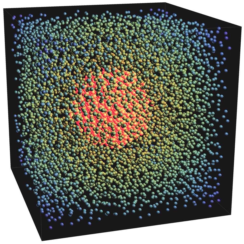
Figure 1: Snapshot of the simulation: the Lennard-Jones atoms in the nanoparticle and the solvent are color-coded in order to visualise the temperature gradient.

In a typical simulation, the system was first equilibrated in the NPT ensemble at the prescribed temperature of $T=0.75$ and pressure of $P=0.01$ using a Nosé–Hoover thermostat and barostat. During the subsequent heating of the nanoparticle to the temperature $T_{\mathrm{p}}$, realised by rescaling the velocities of the atoms belonging to the nanoparticle in each time step, the system evolved in the NPH ensemble, while the particles near the boundary of the simulation box were maintained at $T=0.75$. At least four independent trajectories of $2\cdot 10^{7}$ time steps $\delta t=0.005$ (corresponding to a physical duration of $100$ ns) were computed for each nanoparticle temperature $T_{\mathrm{p}}$. Coordinates and momenta were recorded after attaining stationary thermal conditions. Note that different physical heating mechanisms for the colloidal particle, such as a heat source residing within the particle (which does not directly affect its center-of-mass velocity) versus an external heat supply (which generally does), correspond to different numerical heating procedures.

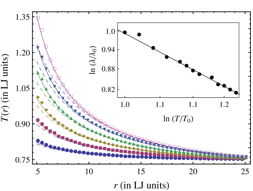
Figure 2: Radial temperature profiles in the cool solvent around a hot nanoparticle of radius $R\approx 5$ for the particle temperatures $T_{\mathrm{p}}=1.00$ $\bullet$, $1.25$ $\blacksquare$, $1.50$ $\diamond$, $1.75$ $\blacktriangle$, $2.00$ $\blacktriangledown$, $2.25$ $\circ$. Dashed and solid lines are fits obtained from Fourier’s law for a thermal conductivity $\lambda\,$=constant (dashed), as assumed in theory, and $\lambda(T)\propto 1/T$, as inferred from the fit to independent simulations of an isothermal bulk fluid (inset), respectively.

Due to the finite compressibility of the Lennard-Jones fluid, the simulation does not comply with the idealizations made in our theoretical calculations (incompressible solvent, constant heat conductivity). Therefore, to accurately describe the temperature profile in the Lennard-Jones solvent (excluding the discontinuity due to the Kaptiza resistance at the particle surface [29]), we need to account for the temperature dependence of the thermal conductivity. Separate simulations of an isothermal bulk fluid along the state-space curve depicted in fig:fig2 (discussed below) yield an inverse temperature dependence for the thermal conductivity, $\lambda\propto 1/T$, as demonstrated in the inset of fig:fig1. The main figure compares the corresponding solution of the heat equation,

$$T(r)=T_{0}\left(1+\Delta T/T_{0}\right)^{\frac{R}{r}}\;,$$ (6)

to the measured temperature profiles around the hot nanoparticle. Here, $T_{0}\approx 0.75$ denotes the nominal ambient temperature at infinite distance $r\to\infty$ from the particle.

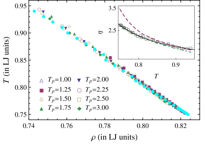
Figure 3: Sample points of the radial temperature and density profiles $T(r)$ and $\rho(r)$ around a hot nanoparticle maintained at various temperatures $T_{\mathrm{p}}$, in the $T-\rho$ plane. The filled circles ($\bullet$) correspond to states for which the viscosity $\eta(T)$ of the bulk Lennard-Jones fluid was determined in separate simulations. The inset compares the latter($\square$) to the empirical formula from eq:etaT_fit (—) and alternative expressions proposed in the recent literature [30] ($\mathbf{--}$) [31] ($\mathbf{-\cdot-}$).

While $T(r)$ can be obtained by averaging the kinetic energy of the solvent particles in the vicinity of $\mathbf{r}$, it is more subtle to deduce the local viscosity $\eta(r)$ from the available microscopic data. Under isothermal conditions, the viscosity can be computed from the microscopic stress tensor $\sigma_{xy}$ via the Green–Kubo formula $\eta=V(k_{\mathrm{B}}T)^{-1}\int_{0}^{\infty}\langle\sigma_{xy}(t)\sigma_{xy}(0)\rangle\,\upd t$. However, the strong temperature gradient in our system precludes the evaluation of the correlation function over a sufficiently large volume to get reliable results. We therefore evaluated the isothermal viscosity $\eta(T)$ of a homogeneous bulk Lennard-Jones fluid with the intention to translate it into $\eta(r)=\eta[T(r)]$ using $T(r)$ from eq:Tr. We observed that the radial dependence of the density $\rho$ around the heated nanoparticle, which is neglected in the analytical calculations, can be quite substantial for the Lennard-Jones fluid. Plotting sample points of the radial temperature and density profiles $T(r)$ and $\rho(r)$ around a heated nanoparticle in the $T-\rho$ plane for various particle temperatures produced the state curve delineated by the data points in fig:fig2. In determining the isothermal bulk viscosity $\eta(T)$ of the Lennard-Jones fluid using to the Green–Kubo formula, we therefore took care to vary the barostat pressure such as to confine the measured bulk states to this curve. In the inset of fig:fig2, we compare our data for $\eta(T)$ to a phenomenological two-parameter fit

$$\ln\left[\eta(T)/\eta_{\infty}\right]=(A/T)^{4}\;.$$ (7)

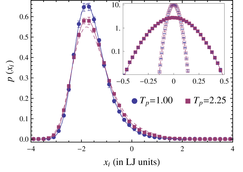
Figure 4: Distribution of the position coordinates of a hot Brownian particle in an asymmetric, anharmonic potential well for two nanoparticle temperatures. The Boltzmann distribution fits the data for the effective temperature $T_{\mathrm{HBM}}$ (solid line) but not for $T_{\mathrm{k}}$ (dashed line), as it should. The inset depicts the distributions of the position (filled symbols) and velocity (open symbols) coordinates in a harmonic well of strength $K=50$ and Boltzmann distributions for the effective temperatures $T_{\mathrm{HBM}}$ (solid line) and $T_{\mathrm{k}}$ (dashed line).

Other observables that can directly be obtained from the simulation are the effective steady-state friction $\zeta_{\mathrm{HBM}}$ and diffusivity $D_{\mathrm{HBM}}$ of the hot Brownian particle. While good estimates for $D_{\mathrm{HBM}}$ are deduced from the nanoparticle trajectories, determining the friction is slightly more subtle [32, 33]. We inferred $\zeta_{\mathrm{HBM}}$ from the decay of the momentum auto-correlation function of the nanoparticle using the Brownian limit [22]. In the simulations, the measured force $\mathbf{F}$ on the colloid does not correspond to the random force $\boldsymbol{\xi}$ entering the Green–Kubo formula for the friction coefficient. From a generalised Langevin description, it can be shown that the correlations $\langle\mathbf{F}(0)\mathbf{F}(t)\rangle$ and $\langle\boldsymbol{\xi}(0)\boldsymbol{\xi}(t)\rangle$ become equal only in the limit of a diverging reduced mass $\mu\to\infty$. The Brownian limit amounts to first taking the mass of the colloidal particle to infinity and then taking the thermodynamic limit of infinitely many solvent particles. As a consequence, the momentum relaxation time of the colloid becomes large compared to the typical relaxation time of the random force autocorrelations, and its momentum autocorrelation function becomes Markovian [32]. It is then found to exhibit an exponential decay

$$\langle\mathbf{P}(t)\mathbf{P}(0)\rangle=\langle\mathbf{P}^{2}(0)\rangle e^{-(\zeta_{\mathrm{HBM}}/\mu)t}$$ (8)

with the decay time determined by the friction coefficient $\zeta_{\mathrm{HBM}}$ and the reduced mass $\mu$. In practice, the Brownian limit is realised following the constrained-dynamics approach [34].

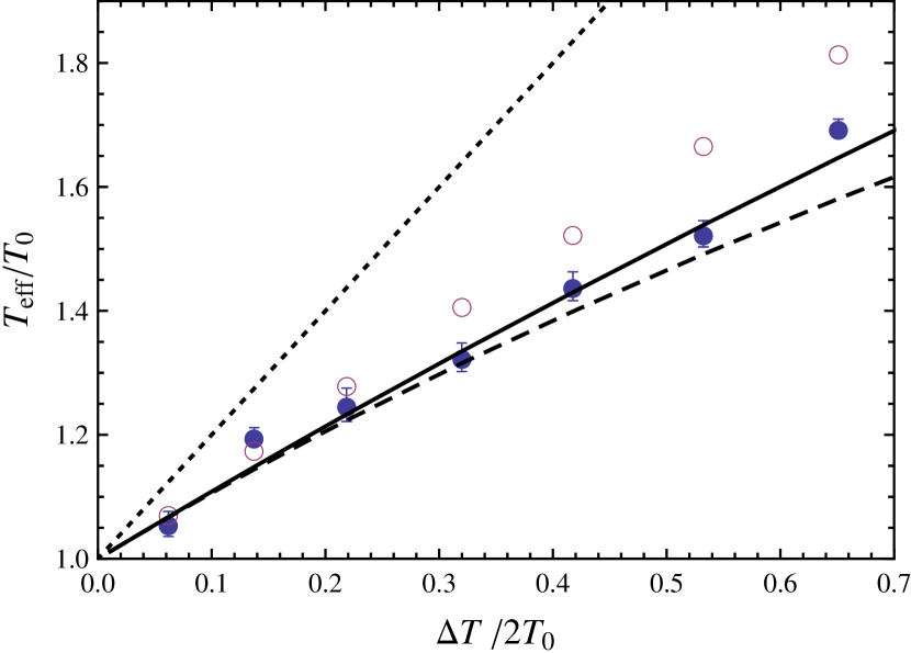
Figure 5: Effective temperatures of translational hot Brownian motion. Simulation: $T_{\mathrm{HBM}}$ ($\bullet$) from the generalised Einstein relation, eq:GER; apparent equipartition temperature $T_{\mathrm{k}}$ ($\circ$) for the particle velocity; solvent temperature at the particle surface (dotted) Theory: $T_{\mathrm{HBM}}$ according to eq:T_HBM_Manuel (solid line) and the previous thermodynamic estimate, eq. (22) of Ref. [14] (dashed line), both evaluated (assuming an incompressible fluid) with the exact numerical differential shell method [14].

Knowing $\zeta_{\mathrm{HBM}}$ and $D_{\mathrm{HBM}}$, we can determine the configurational effective temperature $T_{\mathrm{HBM}}$ using the generalised Einstein relation eq:GER. The temperature $T_{\mathrm{k}}$ for the kinetic degrees of freedom is extracted from the equal-time velocity autocorrelation of the nanoparticle by applying the equipartition relation $\mu\langle\mathbf{U}^{2}\rangle=3k_{B}T_{\mathrm{k}}$. Note, however, that for hot particles, which are far from equilibrium, the pertinence of the equipartition temperature $T_{\mathrm{k}}$ is a priori unclear. We refer the reader to Joly et al. [16] for a discussion of this aspect.

Results and discussion In the remainder of this paper, we present our simulation results for the effective temperatures $T_{\mathrm{HBM}}$ and $T_{\mathrm{k}}$ of translational hot Brownian motion and test our theoretical predictions.

To support the first claim formulated in the introduction, we performed simulations in the presence of external potential forces derived from the harmonic potential $\mathcal{V}(\mathbf{r})=Kr^{2}/2$ for different values of the stiffness parameter $K$. Generalising the corresponding definitions for the free particle, the effective temperatures are inferred from the particle’s mean kinetic energy ($k_{\mathrm{B}}T_{\mathrm{k}}\equiv\mu\langle\mathbf{U}^{2}\rangle/3$) and mean square displacement ($k_{\mathrm{B}}T_{\mathrm{HBM}}\equiv K\langle\mathbf{r}^{2}\rangle/3$) in the harmonic well. In the supplementary online materials[26], they are compared to results for a free Brownian particle maintained at the same temperature to demonstrate perfect agreement to within the statistical errors. In the inset of fig:fig6 it is moreover verified that the coordinates and momenta are indeed Boltzmann distributed with the respective effective temperatures. The main plot demonstrates for two exemplary particle temperatures $T_{\mathrm{p}}$ that this generalises to an asymmetric and anharmonic potential well $\mathcal{V}(\mathbf{r})=\sum_{i=1}^{3}v(x_{i})$ with $v(x)=Kx^{4}/4+bx$. Altogether, the good agreement in all cases confirms that the particle velocity and position are distributed according to effective Boltzmann distributions governed by the same effective temperatures $T_{\mathrm{k}}$ and $T_{\mathrm{HBM}}$ as found for the freely diffusing particle.

To establish also our second claim, fig:fig3 provides a comparison of our theoretical prediction for $T_{\mathrm{HBM}}$ from eq:T_HBM_Manuel and the simulation results obtained by means of the generalised Einstein relation, eq:GER. The good agreement validates eq:GER and eq:T_HBM_Manuel over a wide temperature range. Also note that, at strong heating, eq:T_HBM_Manuel fits the data significantly better than the previous thermodynamic estimate, eq. (22) of Ref. [14]—which amounts to a weighted average of $1/T$ instead of $T$ in eq:T_HBM_Manuel, and is therefore systematically too small. As detailed in the supplementary online materials[26], the configurational temperature $T_{\mathrm{HBM}}$ is found to be insensitive to the precise microscopic conditions such as the particle solubility or the physical realisation of the heating mechanism (internal/external), while $T_{\mathrm{k}}$ is sensitive to the heating mechanism.

In summary, more than a century after Langevin published his famous equation [35], we can now describe the overdamped Brownian motion of a hot nanoparticle by

$$\zeta_{\mathrm{HBM}}\dot{\mathbf{r}}=-\nabla\mathcal{V}(\mathbf{r})+\boldsymbol{\xi}(t)\;.$$ (9)

The effective Gaussian thermal noise $\xi(t)$ is characterised by $\langle\xi(t)\rangle=0$ and $\langle\xi(t)\xi(t^{\prime})\rangle=2T_{\mathrm{HBM}}\zeta_{\mathrm{HBM}}\delta(t-t^{\prime})$. All coefficients are explicitly known over a wide temperature range, and accurate analytical expressions for them have been derived. Most importantly, we have established the following fundamental properties of the effective temperature $T_{\mathrm{HBM}}$ given in eq:T_HBM_Manuel: (1) it governs the Boltzmann factor for the probability distribution of a hot nanoparticle in an external potential $\mathcal{V}(\mathbf{r})$; (2) it may be expressed in terms of the directly measurable effective diffusivity $D_{\mathrm{HBM}}$ and friction $\zeta_{\mathrm{HBM}}$ via the generalised Einstein relation, eq:GER; and (3) it takes distinct values for translational and rotational degrees of freedom [15]. The momenta of the particle were also found to be Boltzmann distributed with and without external potential forces, but according to yet another effective temperature $T_{\mathrm{k}}$ that also takes distinct values for translational and rotational degrees of freedom, and, in contrast to $T_{\mathrm{HBM}}$, is sensitive to the precise heating mechanism. Altogether, our findings strongly support the expectation [1] that the effective temperature $T_{\mathrm{HBM}}$ can be treated as a bona-fide temperature for the configurational Brownian motion of an individual hot particle, and thus pave the way for manifold applications. It remains as an intriguing open question how far this convenient description can be extended to account for finite particle densities, anisotropies, [2] and self-thermophoresis [36].

Supporting Information A PDF file with technical and supplementary information containing a detailed formulation of the contraction of the fluctuating hydrodynamics problem to a Markovian Langevin description of the Brownian motion of the nanoparticle, convenient analytical approximations for $T_{\mathrm{HBM}}$ and $D_{\mathrm{HBM}}$, a discussion of how to obtain $\zeta_{\mathrm{HBM}}$ and how to deal with finite size effects in the numerical simulations, information about the parallel processing of the simulation code, and various supporting plots is available free of charge via the Internet at http://arxiv.org/…