Particle injection into a chain: decoherence versus relaxation for Hermitian and non-Hermitian dynamics

Abstract

We investigate a model system for the injection of fermionic particles from filled source sites into an empty chain. We study the ensuing dynamics for Hermitian as well as for non-Hermitian time evolution where the particles cannot return to the bath sites (quantum ratchet). A non-homogeneous hybridization between bath and chain sites permits transient currents in the chain. Non-interacting particles show decoherence in the thermodynamic limit: the average particle number and the average current density in the chain become stationary for long times, whereas the single-particle density matrix displays large fluctuations around its mean value. Using the numerical time-dependent density-matrix renormalization group ($t$-DMRG) method we demonstrate, on the other hand, that sizable density-density interactions between the particles introduce relaxation which is by orders of magnitudes faster than the decoherence processes.

1 Introduction

Newton’s equations describe the deterministic time evolution of a given initial state of classical particles. In principle, the particle velocities and positions are known for all times. In practice, in isolated systems and for long times, macroscopic observables which involve the averages over many particles can be calculated equally accurately starting from thermodynamic considerations. The ‘thermalization’ of macroscopic systems is one of the building principles of statistical mechanics. According to statistical mechanics, expectation values for macroscopic observables should, for long times, become independent of time and, moreover, become equal to their statistical average; for a recent example of the relaxation of classical particles in a one-dimensional box, see Ref. [1]. The ‘thermalization principle’ equally applies to quantum mechanics where the Schrödinger equation describes the deterministic evolution of a given initial state in time. Recently, the question under which conditions thermalization is possible in closed quantum systems has also been studied, both experimentally and theoretically [2, 3, 4]. According to the eigenstate thermalization hypothesis, each generic state of a closed quantum system already contains a thermal state which is revealed during unitary time evolution due to dephasing and relaxation processes. However, proofs for this hypothesis have so far only been obtained in very specific settings [5, 6]; its applicability for generic quantum systems remains a matter of current research.

In this work, we are interested in the quantum-mechanical injection of particles into a chain. For this toy model we can study the approach to a steady state analytically and numerically. The time evolution of prepared initial states in one-dimensional quantum systems such as our toy model can be studied experimentally using cold atomic gases on optical lattices confined to one dimensional potentials [2, 3, 7, 8]. These systems are to a very high degree isolated from the environment and are therefore ideally suited to study non-equilibrium dynamics in closed quantum systems. Besides the Hermitian time evolution we also address the non-Hermitian case for our toy model where the chain particles cannot return to the bath sites (a ‘quantum ratchet’ [9, 10]). In general, effective non-Hermitian Hamiltonians are naturally obtained if one simulates a dissipative environment for a quantum model in the form of a Lindblad equation [11]. An effective non-Hermitian Hamiltonian has also been used to study the depinning of flux lines in superconductors [12]. Interesting from a fundamental point of view are, in particular, so-called pseudo-Hermitian Hamiltonians—including Hamiltonians having $\mathcal{PT}$-symmetry—which have real spectra and therefore offer a natural framework to extend standard quantum mechanics [13, 14, 15].

In Sect. 2 we recapitulate the Schrödinger equation for time evolution in quantum mechanics. We treat both cases of Hermitian and non-Hermitian Hamilton operators. In Sect. 3 we introduce our model system for spinless fermions. We consider a chain of sites which is initially empty and is coupled to initially filled bath sites. At finite times, the hybridization introduces particles in the chain where they can move between neighboring sites. The hybridizations can be homogenous or inhomogeneous; in the latter case they induce a transient current in the chain.

In Sect. 4 we discuss the particle density, the single-particle density matrix, and the current density for non-interacting fermions. In the thermodynamic limit, the particle and current densities become constant for large times because the contributions of individual modes interfere destructively (‘decoherence’). The oscillations in the single-particle density matrix on the other hand reveal the absence of relaxation for non-interacting particles. Furthermore, we investigate the influence of the ratchet condition on the chain dynamics. In Sect. 5 we include a density-density interaction between the particles. We use the time-dependent density-matrix renormalization group ($t$-DMRG) method to evolve the quantum-mechanical states in time. The interaction between the particles induces a fast relaxation to stationary distributions for the particle density, single-particle density matrix, and current. For our model system, with interactions of the order of the bandwidth, we find that the relaxation time scale is two orders of magnitude shorter than the time scale for dephasing.

A summary and conclusions, Sect. 6 , close our presentation. Calculations for the asymmetric chain filling in the ratchet case are deferred to appendix A.

2 Hermitian and non-Hermitian time evolution

We begin our discussion with the Schrödinger equation which defines the time evolution for Hermitian and non-Hermitian Hamilton operators. As in standard quantum mechanics, expectation values are to be taken using the time-dependent wave function. The von-Neumann equation of motion of the corresponding statistical operator can be cast into the general form of a Kossakowski–Lindblad equation.

2.1 Schrödinger equation

We consider a finite-dimensional Hilbert space $\mathbb{V}$. Its elements are the states $|\psi\rangle$. We use the standard scalar product $\langle\phi|\psi\rangle\in\mathbb{C}$ where $\langle\phi|$ is the shorthand notation for the linear functionals $\langle\phi|\cdot\rangle$ which form the dual space $\mathbb{V}^{*}$ of our Hilbert space. For an operator $\hat{O}$ which acts in $\mathbb{V}$, its adjoint $\hat{O}^{\dagger}$ is defined by $\langle\phi|\hat{O}^{\dagger}|\psi\rangle=\langle\psi|\hat{O}|\phi\rangle^{*}$ for all $\langle\phi|\in\mathbb{V}^{*}$ and $|\psi\rangle\in\mathbb{V}$ where $z^{*}$ is the complex conjugate of $z\in\mathbb{C}$.

For time $t\geq 0$, the time evolution of a state $|\psi\rangle$ and of its adjoint state $\langle\psi|$ is given by

$$|\psi(t)\rangle=\exp\left(-{\rm i}\hat{H}t\right)|\psi\rangle\quad,\quad\langle\psi(t)|=\langle\psi|\exp\left({\rm i}\hat{H}^{\dagger}t\right)\;,$$ (2.1)

where $\hat{H}$ is a time-independent Hamilton operator and $\hat{H}^{\dagger}$ is its adjoint.

In the following we shall assume that the spectrum of $\hat{H}$ is real, i.e., the eigenstates of $\hat{H}$ obey

$$\hat{H}|E_{n}\rangle=E_{n}|E_{n}\rangle\quad(n=1,2,\ldots)$$ (2.2)

with $E_{n}\in\mathbb{R}$. As shown in Ref. [13] this implies that $\hat{H}$ is pseudo-Hermitian and $\hat{H}^{\dagger}$ has the same spectrum,

$$\hat{H}^{\dagger}|\overline{E_{n}}\rangle=E_{n}|\overline{E_{n}}\rangle\quad(n=1,2,\ldots)\;.$$ (2.3)

Eq. (2.3) implies that there is a left eigenvector $\langle\overline{E_{n}}|$ of $\hat{H}$ for every right eigenvector $|E_{n}\rangle$ of $\hat{H}$ with the same eigenvalue $E_{n}$.

Note that $\langle\overline{E_{n}}|=\left(|E_{n}\rangle\right)^{\dagger}$ only if $\hat{H}$ is Hermitian, $\hat{H}^{\dagger}=\hat{H}$. The eigenstates of $\hat{H}$ and $\hat{H}^{\dagger}$ for different energies are orthogonal $\langle\overline{E_{n}}|E_{m}\rangle=0$ if $E_{n}\neq E_{m}$. Using proper linear combinations of eigenstates for degenerate eigenvalues we can write for the Hamiltonian, its adjoint, and the unit operator

$$\hat{H}=\sum_{n}E_{n}|E_{n}\rangle\langle\overline{E_{n}}|\quad,\quad\hat{H}^{\dagger}=\sum_{n}E_{n}|\overline{E_{n}}\rangle\langle E_{n}|\quad,\quad\hat{1}=\sum_{n}|\overline{E_{n}}\rangle\langle E_{n}|=\sum_{n}|E_{n}\rangle\langle\overline{E_{n}}|=\hat{1}^{\dagger}\;,$$ (2.4)

where $\langle\overline{E}_{n}|E_{n}\rangle=1$ thus forming a biorthonormal set of eigenvectors. The Hamiltonian and its adjoint obey the (pseudo-)Hermiticity condition [13]

$$\hat{\eta}\hat{H}=\hat{H}^{\dagger}\hat{\eta}\quad,\quad\hat{\eta}=\sum_{n}|\overline{E_{n}}\rangle\langle\overline{E_{n}}|=\hat{\eta}^{\dagger}\quad,\quad\hat{\eta}^{-1}=\sum_{n}|E_{n}\rangle\langle E_{n}|\;.$$ (2.5)

Note that all definitions reduce to the standard expressions in the case of Hermitian time evolution with $\hat{H}=\hat{H}^{\dagger}$ and $\hat{\eta}=\hat{1}$.

2.2 Measurements

In standard quantum mechanics, the expectation value for an operator $\hat{O}$ is given by

$$\langle\hat{O}\rangle(t)=\frac{\langle\psi(t)|\hat{O}|\psi(t)\rangle}{\langle\psi(t)|\psi(t)\rangle}\;.$$ (2.6)

For pseudo-Hermitian time evolution, this definition remains unchanged. It is important to note that the time evolution described by (2.1) is not unitary so that the norm $\langle\psi(t)|\psi(t)\rangle$ is not conserved and must be considered separately.

As a consequence, the equation of motion for the statistical operator changes its form. The statistical operator for the pure state $|\psi(t)\rangle$ is defined by

$$\hat{\rho}(t)=\frac{|\psi(t)\rangle\langle\psi(t)|}{\langle\psi(t)|\psi(t)\rangle}\;.$$ (2.7)

With the help of the statistical operator, expectation values can be expressed in the form

$$\langle\hat{O}\rangle(t)={\rm Tr}\bigl{(}\hat{\rho}(t)\hat{O}\bigr{)}\;.$$ (2.8)

where ${\rm Tr}$ denotes the trace which implies the sum over the expectation values of an orthonormal basis set. The statistical operator obeys $\hat{\rho}^{\dagger}=\hat{\rho}$, $\hat{\rho}^{2}=\hat{\rho}$ and ${\rm Tr}\hat{\rho}=1$. Its time dependence is given by the equation of motion (generalized von Neumann equation)

$${\rm i}\frac{{\rm d}}{{\rm d}t}\hat{\rho}(t)=\hat{H}\hat{\rho}(t)-\hat{\rho}(t)\hat{H}^{\dagger}+\hat{\rho}(t)\langle\hat{H}^{\dagger}-\hat{H}\rangle(t)\;.$$ (2.9)

When we split the Hamiltonian into a Hermitian part $\hat{H}_{0}=\hat{H}_{0}^{\dagger}$ and a non-Hermitian perturbation $\hat{V}\neq\hat{V}^{\dagger}$ we can equivalently write

$$\frac{{\rm d}}{{\rm d}t}\hat{\rho}(t)=-{\rm i}\left[\hat{H}_{0},\hat{\rho}(t)\right]_{-}-{\rm i}\left(\bigl{(}\hat{V}-\langle\hat{V}\rangle(t)\bigr{)}\hat{\rho}(t)-\hat{\rho}(t)\bigl{(}\hat{V}^{\dagger}-\langle\hat{V}^{\dagger}\rangle(t)\bigr{)}\right)\;.$$ (2.10)

Apparently, the generalized von-Neumann equation takes the form of the Kossakowski–Lindblad equation [16, 17].

3 Particle injection into a chain

As an example we study the injection of fermionic particles from filled source sites into an empty chain. We start with a translationally invariant coupling of the source and bath sites. Next, we consider an inhomogeneous coupling which permits us to generate a transient current density in the chain. For the case of non-interacting fermions, analytical expressions can be worked out for the particle density, the single-particle density matrix, and the current density. For interacting fermions, we evolve the states in time with the density-matrix renormalization group ($t$-DMRG) method.

3.1 Hamilton operator

We consider a finite chain with $L$ sites on which spinless fermions can move between neighboring sites,

$$\hat{T}=-J\sum_{l=1}^{L-1}\left(\hat{c}_{l+1}^{\dagger}\hat{c}_{l}+\hat{c}_{l}^{\dagger}\hat{c}_{l+1}\right)\;,$$ (3.1)

where $\hat{c}_{l}^{\dagger}$ ($\hat{c}_{l}$) creates (annihilates) a fermion at site $l$. Later, we will set $J=1$ as our energy unit (bare bandwidth $W=4$).

The chain fermions are locally hybridized with reservoir fermions,

$$\hat{S}=\sum_{l=1}^{L}\left(\gamma_{l,{\rm in}}\hat{c}_{l}^{\dagger}\hat{s}_{l}+\gamma_{l,{\rm out}}\hat{s}_{l}^{\dagger}\hat{c}_{l}\right)\;.$$ (3.2)

The hybridization strength for the fermion transfer from the reservoir to the chain, $\gamma_{l,{\rm in}}$, can be different from the transfer from the chain to the reservoir, $\gamma_{l,{\rm out}}$. In this work we focus on the Hermitian case, $\gamma_{l,{\rm in}}=\gamma_{l,{\rm out}}$, and the ratchet case, $\gamma_{l,{\rm out}}=0$, where the chain fermions cannot return to the reservoir sites. We will study the translationally invariant case, $\gamma_{l,{\rm in}}=\gamma$, and the inhomogeneous case with $\gamma_{l+1,{\rm in}}<\gamma_{l,{\rm in}}=J\exp(-l/L)$.

In Sect. 5 we consider numerically the time evolution in the presence of density-density interactions between the fermions,

$$\hat{V}=\sum_{l}V_{\rm c}\bigl{(}\hat{c}_{l}^{\dagger}\hat{c}_{l}-\frac{1}{2}\bigr{)}\bigl{(}\hat{c}_{l+1}^{\dagger}\hat{c}_{l+1}-\frac{1}{2}\bigr{)}+V_{\rm s}\bigl{(}\hat{s}_{l}^{\dagger}\hat{s}_{l}-\frac{1}{2}\bigr{)}\bigl{(}\hat{s}_{l+1}^{\dagger}\hat{s}_{l+1}-\frac{1}{2}\bigr{)}+V_{\rm cs}\bigl{(}\hat{c}_{l}^{\dagger}\hat{c}_{l}-\frac{1}{2}\bigr{)}\bigl{(}\hat{s}_{l}^{\dagger}\hat{s}_{l}-\frac{1}{2}\bigr{)}\;.$$ (3.3)

All interaction parameters are chosen to be positive. The total Hamiltonian is given by

$$\hat{H}=\hat{T}+\hat{S}+\hat{V}\;.$$ (3.4)

The model is shown pictorially in Fig. 1.

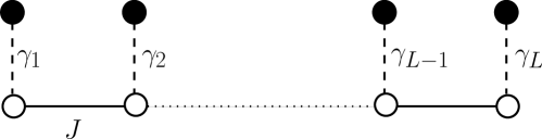
Figure 1: Model for the particle injection into a chain. The solid circles represent the source sites, the open circles the chain sites. The solid and dashed lines denote the bonds with hopping amplitudes $J$ and $\gamma_{l}$ respectively.

3.2 Initial state and measured quantities

In order to study the particle injection from the reservoir into the chain, we choose our initial state as

$$|\psi(t=0)\rangle=|\psi_{0}\rangle=\prod_{l=1}^{L}\hat{s}_{l}^{\dagger}|{\rm vac}\rangle\;.$$ (3.5)

At time $t=0$ all source sites are occupied and the chain is empty.

We are interested in the average particle density in the chain, $n_{c}(t)$, the single-particle density matrix of the chain fermions, $A_{p,k}(t)$, and the current density, $j_{c}(t)$. These quantities are defined by

$$A_{p,k}(t) = \langle\hat{a}_{p}^{\dagger}\hat{a}_{k}\rangle(t)\quad,\quad\hat{a}_{k}=\sqrt{\frac{2}{L+1}}\sum_{l=1}^{L}\sin\left(\frac{\pi kl}{L+1}\right)\hat{c}_{l}\quad(k=1,2,\ldots,L)\;,$$

$$n_{c}(t) = \frac{1}{L}\sum_{k=1}^{L}A_{k,k}(t)\;,$$ (3.6)

$$j_{c}(t) = \frac{{\rm i}}{L}\sum_{l=1}^{L-1}\langle\hat{c}_{l+1}^{\dagger}\hat{c}_{l}-\hat{c}_{l}^{\dagger}\hat{c}_{l+1}\rangle(t)=-\frac{2{\rm i}}{L+1}\sum_{\begin{subarray}{c}p,k=1\\ p\neq k\end{subarray}}^{L}j(k,p)A_{p,k}(t)\;,$$

$$j(k,p) = \frac{(1-(-1)^{p-k})}{L}\frac{\sin\bigl{(}p\pi/({L+1})\bigr{)}\sin\bigl{(}k\pi/({L+1})\bigr{)}}{\cos\bigl{(}k\pi/({L+1})\bigr{)}-\cos\bigl{(}p\pi/({L+1})\bigr{)}}\;.$$

For a homogeneous coupling, $\gamma_{l}=\gamma$, the single-particle density matrix is diagonal, $A_{p,k}(t)=\delta_{k,p}A_{k,k}$, and the current density is zero for all times, $j_{c}(t)=0$.

The long-time mean of a time-dependent quantity $X(t)$ is defined as

$$\overline{X(t)}=\lim_{\tau\to\infty}\frac{1}{\tau}\int_{0}^{\tau}X(t){\rm d}t\;.$$ (3.7)

4 Non-interacting fermions

First, we address the question of how effective the injection of non-interacting fermions into the empty chain is. To this end, we consider the average particle number, the single-particle density matrix, and the current density in the chain, as functions of time.

At short times we expect a linear increase of the particle density in the chain because we start with all particles at the source sites. At later times, we shall see an oscillatory behavior of the particle density because of the coherent quantum-mechanical movement of the particles within and into the chain (and back onto the source sites for the Hermitian case). In the non-interacting case, a constant average occupation is reached only for long times because the two-level systems stay coherent for relatively long times so that the oscillations in the particle density die out only slowly. Interactions dampen these oscillations strongly and also modify the value in the long-time limit considerably, see Sect. 5.

4.1 Homogeneous chain filling

We begin with the translationally invariant case for non-interacting particles, $\gamma_{l,{\rm in}}=\gamma_{\rm in}$ and $\gamma_{l,{\rm out}}=\gamma_{\rm out}$ in eq. (3.2). For a homogeneous chain filling, the single-particle density matrix is diagonal and the current density is zero for all times.

4.1.1 Hermitian time evolution

In the Hermitian time evolution with $\gamma_{\rm in}=\gamma_{\rm out}=\gamma$ the model reads

$$\hat{H}=-J\sum_{j=1}^{L-1}[\hat{c}^{\dagger}_{j+1}\hat{c}_{j}+\hat{c}^{\dagger}_{j+1}\hat{c}_{j}]+\gamma\sum_{j=1}^{L}[\hat{s}^{\dagger}_{j}\hat{c}_{j}+\hat{c}^{\dagger}_{j}\hat{s}_{j}]=\sum_{k}[\varepsilon_{k}\hat{a}^{\dagger}_{k}\hat{a}_{k}+\gamma(\hat{a}^{\dagger}_{k}\hat{b}_{k}+\hat{b}^{\dagger}_{k}\hat{a}_{k})]\;,$$ (4.1)

where $\hat{b}_{k}$ denotes the Fourier transform of the operators $\hat{s}_{l}$ defined analogously to the Fourier transform of the chain operators in eq. (3.6). The dispersion is given by $\varepsilon_{k}=-2J\cos k$ with $k=\pi n/(L+1)$.

Heisenberg’s equations of motion provide the simplest way to solve this problem analytically. The resulting coupled differential equations read

$$\dot{\hat{a}}_{k} = {\rm i}[\hat{H},\hat{a}_{k}]=-{\rm i}(\varepsilon_{k}\hat{a}_{k}+\gamma\hat{b}_{k})\quad\textrm{and}$$

$$\dot{\hat{b}}_{k} = {\rm i}[\hat{H},\hat{b}_{k}]=-{\rm i}\gamma\hat{a}_{k}\;.$$ (4.2)

It is straightforward to write down a formal solution,

$$\begin{pmatrix}\hat{a}_{k}(t)\\ \hat{b}_{k}(t)\end{pmatrix}=e^{-{\rm i}\mathbf{\widetilde{M}_{k}}t}\begin{pmatrix}\hat{a}_{k}\\ \hat{b}_{k}\end{pmatrix}\;,$$ (4.3)

where

$$\mathbf{\widetilde{M}_{k}}=\begin{pmatrix}\varepsilon_{k}&\gamma\\ \gamma&0\end{pmatrix}\;.$$ (4.4)

Re-expressing the exponential matrix leads to

$$\begin{pmatrix}\hat{a}_{k}(t)\\ \hat{b}_{k}(t)\end{pmatrix}=e^{-{\rm i}\varepsilon_{k}t/2}\mathbf{M_{k}}(t)\begin{pmatrix}\hat{a}_{k}\\ \hat{b}_{k}\end{pmatrix}$$ (4.5)

with

$$M_{k,11}=M_{k,22}^{*} = \cos\left(E_{k}t/2\right)-{\rm i}\frac{\varepsilon_{k}\sin\left(E_{k}t/2\right)}{E_{k}}\;,$$

$$M_{k,12}=M_{k,21} = -{\rm i}\frac{2\gamma}{E_{k}}\sin\left(E_{k}t/2\right)\;,$$ (4.6)

$$E_{k} = \sqrt{\varepsilon_{k}^{2}+4\gamma^{2}}\;.$$

The zero-time correlation functions are very simple,

$$\langle\psi_{0}|\hat{a}^{\dagger}_{k}\hat{a}_{k}|\psi_{0}\rangle=\langle\psi_{0}|\hat{a}^{\dagger}_{k}\hat{b}_{k}|\psi_{0}\rangle=0\quad,\quad\langle\psi_{0}|\hat{b}^{\dagger}_{k}\hat{b}_{k}|\psi_{0}\rangle=1\;.$$ (4.7)

The single-particle density matrix is diagonal and given by

$$A_{k,k}(t)=\left|M_{k,12}\right|^{2}=\frac{4\gamma^{2}}{E_{k}^{2}}\sin^{2}\left(E_{k}t/2\right)\;.$$ (4.8)

It describes the beating of particles in the two-level systems with energies $\varepsilon_{k;1,2}=(1/2)(\varepsilon_{k}\pm E_{k})$ which result from the hybridization of the bath particles at zero energy with the chain particles with dispersion $\varepsilon_{k}$.

The average particle number in the chain becomes

$$n_{c}(t)=\frac{1}{L}\sum_{k}\frac{4\gamma^{2}}{E_{k}^{2}}\sin^{2}\left(E_{k}t/2\right)\;.$$ (4.9)

Its long-time mean is straightforwardly extracted,

$$\overline{n_{c}(t)}=\frac{1}{2L}\sum_{k}\frac{4\gamma^{2}}{E_{k}^{2}}\;.$$ (4.10)

In principle, the oscillations around the mean will not die out for long times. For any finite chain there exists a recurrence time $t^{\epsilon}_{\rm rec}\neq 0$ such that for the numerator of the sum (4.9) the relation $\sin^{2}(t^{\epsilon}_{\rm rec}E_{k}/2)<\epsilon/L$ holds for all allowed $k$-values. However, this Poincaré time is very large even for systems $L=50$ because the energies $E_{k}$ are not commensurate.

In the thermodynamic limit ($L\to\infty$) eq. (4.9) reduces to

$$n_{c}(t)=\frac{2}{\pi}\int_{0}^{J/\gamma}\frac{{\rm d}\varepsilon}{\sqrt{(J/\gamma)^{2}-\varepsilon^{2}}}\frac{\sin^{2}(\gamma t\sqrt{1+\varepsilon^{2}})}{1+\varepsilon^{2}}\;.$$ (4.11)

In this case the oscillations in $n_{c}(t)$ do vanish for $t\to\infty$ because the infinitely many two-level systems dephase completely. We find

$$n_{c}(t\to\infty)=\frac{1}{2}\frac{1}{\sqrt{1+(J/\gamma)^{2}}}\;.$$ (4.12)

For $J/\gamma\to 0$ only half of the chain sites are occupied on average. Recall that, for $J=0$, we describe a collection of independent two-level systems where each particle oscillates between two levels such that it is equally likely to be found on the chain and on the bath site.

For $J/\gamma\ll 1$, the integral (4.11) can be solved to leading order,

$$n_{c}(t)\approx\frac{1}{2}-\frac{1}{2}J_{0}(tJ^{2}/(2\gamma))\left[\cos(2\gamma t)\cos(tJ^{2}/(2\gamma))+\sin(2\gamma t)\sin(tJ^{2}/(2\gamma))\right]\;.$$ (4.13)

Here, the trigonometric functions describe the fast oscillations around the mean value whereas the Bessel function $J_{0}(tJ^{2}/2\gamma)$ gives the envelope. The oscillations around the mean value decay in the long time limit proportional to $\sqrt{2\gamma/J^{2}t}$. The slow oscillatory decay proportional to $1/\sqrt{t}$ results from the square-root divergence in the single-particle density of states in one dimension.

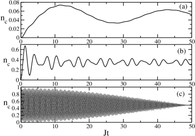
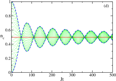
Figure 2: Particle density in the chain $n_{c}(t)$ for non-interacting fermions (Hermitian time evolution). Left: a chain with $L=50$ sites and (a) $\gamma/J=0.1$, (b) $\gamma/J=1$, (c) $\gamma/J=10$; (d): thermodynamic limit for $\gamma/J=10$ (circles: time steps $\delta t=0.1$). The solid line is the long-time limit, the dashed lines show the envelope function according to eq. (4.13).

In Fig. 2 we show results for different ratios of $\gamma/J$ for a chain with $L=50$ sites for times $Jt\leq 50$. For a finite chain, the average particle number will never become constant. Instead, revival oscillations will occur because the Hilbert space has a finite dimension. In the thermodynamic limit, the oscillations slowly decay to a constant average particle number in the chain given by eq. (4.11), see Fig. 2(d), plotted for $\gamma/J=10$ and times $Jt\leq 500$.

As a comparison, we show results for the ratchet case in Fig. 3 for the same values of $\gamma_{\rm in}=\gamma$ ($\gamma_{\rm out}=0$) and different time spans. Even in the ratchet case, not all particles are injected into the chain at long times. Only for $\gamma_{\rm in}\to\infty$ does the particle number in the chain approach unity, see eq. (4.19). In addition, one still observes fluctuations so that the particle density in the chain is not a monotonically increasing function. The motion of the fermions on the chain leads to Pauli blocking and to quantum-mechanical interference effects which result in the observed incomplete and oscillatory chain filling. In comparison with the Hermitian time evolution it can be seen that in the ratchet case the quantum-mechanical fluctuations are smaller and the chain filling is bigger for the same parameter $\gamma/J$.

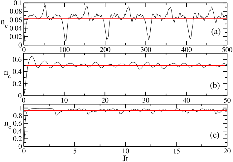
Figure 3: Particle density in the chain $n_{c}(t)$ for non-interacting fermions on a chain with $L=50$ sites for (a) $\gamma_{\rm in}/J=0.1$, (b) $\gamma_{\rm in}/J=1$, and (c) $\gamma_{\rm in}/J=10$ (ratchet time evolution). The straight lines denote the mean values. Note the different scales on the axis.

In Fig. 4 we show the single-particle density matrix $A_{k,k}$ for Hermitian time evolution with $\gamma/J=1$ at various times. At small times all particles enter the chain at roughly the same moment which leads to a relatively flat distribution for $Jt=1$. At larger times, the individual dynamics of each $k$-point becomes visible and a lot of maxima and minima have developed already by $Jt=50$. At very large times, $Jt=5000$, the map $A_{k,k}(t)$, corresponding to a large collection of undamped oscillators, displays a non-monotonic (“chaotic”) distribution. The size of the fluctuations around the time-averaged distribution is as large as its mean. The system does not relax.

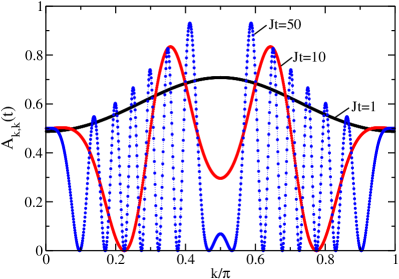
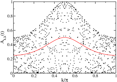
Figure 4: Density matrix $A_{k,k}(t)$ in the Hermitian time evolution with $\gamma/J=1$ for a chain of length $L=1000$ as a function of the discrete momenta $k=\pi n/(L+1)$ for times $Jt=1,10,50$ (left) and $Jt=5000$ (right) where the solid line is the long-time mean.

The corresponding results for the single-particle density matrix $A_{k,k}$ for non-interacting electrons in the ratchet case are shown in Fig. 5. The average distribution is sharply peaked at $k=\pi/2$, see eq. (4.18). This means that for large times the $k$-points near $\pi/2$ show very little variation with time while the $k$-points away from $\pi/2$ are still strongly oscillating in time.

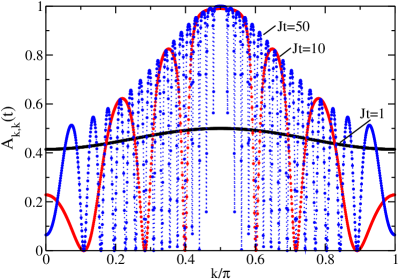
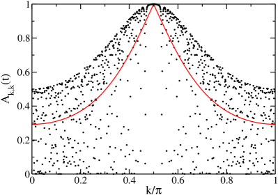
Figure 5: Density matrix $A_{k,k}(t)$ in the ratchet case with $\gamma_{\rm in}/J=1$ for a chain of length $L=1000$ as a function of the discrete momenta $k=\pi n/(L+1)$ for times $Jt=1,10,50$ (left) and $Jt=5000$ (right) where the solid line is the long-time mean.

4.1.2 Ratchet case

Here we provide the analytical expressions on which the data in Figs. 3 and 5 are based. We treat the translationally invariant ratchet case, $\gamma_{l,{\rm out}}=0$ and $\gamma_{l,{\rm in}}=\gamma$. The Fourier transformed Hamiltonian reads

$$\hat{H}=\sum_{k}[\varepsilon_{k}\hat{a}^{\dagger}_{k}\hat{a}_{k}+\gamma\hat{a}^{\dagger}_{k}\hat{b}_{k}]\equiv\hat{H}_{0}+\hat{S}\;,$$ (4.14)

where $\hat{H}_{0}$ is the Hermitian and $\hat{S}$ is the non-Hermitian part. In the interaction picture representation we find

$$\hat{S}(t)=\gamma\sum_{k}e^{{\rm i}\varepsilon_{k}t}\hat{a}^{\dagger}_{k}\hat{b}_{k}\;.$$ (4.15)

In this case one can explicitly calculate the $S$-matrix because $\hat{S}(t)$ commutes with itself at different times and therefore one can directly integrate over times in $\hat{S}(t)$. The wave function becomes

$$|\psi(t)\rangle=\prod_{k=1}^{L}\left(1+\gamma g_{k}(t)\hat{b}_{k}\hat{a}_{k}^{\dagger}\right)|\psi(0)\rangle\quad,\quad g_{k}(t)=\frac{1-e^{-{\rm i}\varepsilon_{k}t}}{\varepsilon_{k}}\;.$$ (4.16)

For the single-particle density matrix we find

$$A_{k,k}(t)=\frac{\gamma^{2}|g_{k}(t)|^{2}}{1+\gamma^{2}|g_{k}(t)|^{2}}=\frac{\sin^{2}(\varepsilon_{k}t/2)}{\varepsilon_{k}^{2}/(4\gamma^{2})+\sin^{2}(\varepsilon_{k}t/2)}\;.$$ (4.17)

In contrast to the Hermitian time evolution, the bare energy levels of the bath and the chain fermions do not hybridize. Therefore, the bare dispersion $\varepsilon_{k}$ appears as the beating frequency. Also note the time-dependence of the denominator which is absent for the Hermitian time evolution, see eq. (4.8).

Again, we note that it is always possible to find a recurrence time $t^{\epsilon}_{\rm rec}$ such that the average particle number in the chain $n_{c}(t^{\epsilon}_{\rm rec})=\sum_{k}A_{k,k}(t^{\epsilon}_{\rm rec})/L<\epsilon$ for any given $\epsilon$. At first, these recurrences seem counter-intuitive because, in the ratchet case, the amplitude for particles going back from the chain onto the source sites is zero. This clearly demonstrates the quantum character of the problem.

The time averaged distribution function is given by

$$\overline{A_{k,k}(t)}=1-\frac{|\epsilon_{k}|}{E_{k}}\;,$$ (4.18)

which is sharply peaked at $k=\pi/2$. In the thermodynamic limit we therefore find that the density of particles in the chain is given by

$$n_{c}(t\to\infty)=1-\frac{2}{\pi}\arctan\left(\frac{J}{\gamma}\right)\;.$$ (4.19)

For a collection of independent two-level systems of bath and chain sites ($J=0$), the chain is completely filled for large times because the particles cannot return to the bath sites. For $J/\gamma\neq 0$, however, we have $n_{c}(t\to\infty)<1$, i.e., the chain is not completely filled despite the ratchet condition. Due to the motion of the particles on the chain, some bath particles are prevented from falling down into the chain because their chain sites are blocked by other particles (Pauli exclusion principle).

4.2 Inhomogeneous chain filling

For an inhomogeneous coupling, the problem must be treated numerically. It involves the diagonalization of the Hamiltonian (Hermitian time evolution) or the inversion of the self-energy matrix (ratchet case).

4.2.1 Hermitian time evolution

We rewrite the Hamilton operator as

$$\hat{H}=\sum_{i,j=1}^{2L}H_{i,j}\hat{p}_{i}^{\dagger}\hat{p}_{j}$$ (4.20)

with $\hat{p}_{2m-1}=\hat{s}_{m}$, $\hat{p}_{2m}=\hat{c}_{m}$ for $m=1,2,\ldots,L$ and $H_{2m-1,2m}=H_{2m,2m-1}=\gamma_{m}$, $H_{2m+2,2m}=H_{2m,2m+2}=-J$ for $m=1,2,\ldots,L-1$. The Hamiltonian is diagonal in a new single-particle basis,

$$\hat{H}=\sum_{N=1}^{2L}E_{N}\hat{\xi}_{N}^{\dagger}\hat{\xi}_{N}\quad,\quad\hat{\xi}_{N}=\sum_{j=1}^{2L}U_{j,N}\hat{p}_{j}\quad,\quad\hat{p}_{j}=\sum_{N=1}^{2L}U^{*}_{j,N}\hat{\xi}_{N}=\sum_{N=1}^{2L}U_{j,N}\hat{\xi}_{N}\;,$$ (4.21)

where we used in the last step that the transformation matrix $U$, which is determined numerically, is real. The single-particle density matrix in momentum space is best calculated from the corresponding expression in position space,

$$A_{p,q}(t)=\sum_{l,r}\frac{2}{L+1}\sin\left(\frac{\pi pl}{L+1}\right)\sin\left(\frac{\pi qr}{L+1}\right)C_{l,r}(t)$$ (4.22)

with

$$C_{l,r}(t) = \langle\psi(t)|\hat{p}_{2l}^{\dagger}\hat{p}_{2r}|\psi(t)\rangle$$ (4.23)

$$= \sum_{N,M=1}^{2L}e^{{\rm i}(E_{N}-E_{M})t}\left(\sum_{m=1}^{L}U_{2m-1,N}U_{2m-1,M}\right)U_{2l,N}U_{2r,M}\;.$$

Here we used the time evolution (2.1) and the fact that all bath sites are occupied at time $t=0$ so that $\langle\psi(0)|\hat{p}_{2m-1}^{\dagger}\hat{p}_{2n-1}|\psi(0)\rangle=\delta_{m,n}$. The calculation of $A_{p,q}(t)$ involves five lattice summations which are performed numerically.

For an inhomogeneous coupling, $\gamma_{l}=J\exp(-l/L)$, the particle-density in the chain $n_{c}(t)$ is qualitatively similar to the case of a symmetric filling for $\gamma=J$. In Fig. 6, we show the filling of the chain for the unitary time evolution and the ratchet case for times $Jt\leq 100$.

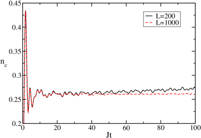
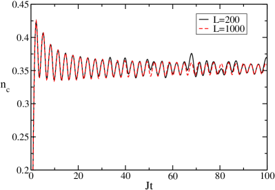
Figure 6: Particle density in the chain $n_{c}(t)$ for non-interacting fermions with hopping $\gamma_{l}=J\exp(-l/L)$ on a chain with $L=200$ ($L=1000$) sites for unitary time evolution (left) and ratchet time evolution (right).

In the unitary case, the fluctuations in the particle density are much smaller for the inhomogeneous hybridizations than for constant hybridizations. In addition, larger system sizes reduce the fluctuations further as can be seen from the comparison for system sizes $L=200$ and $L=1000$. In any case the particle density reaches its long-time value for times $Jt\gtrsim 1000$ with small fluctuations around it. These reflect the transient current density in the system, see Fig. 8. In the ratchet case, we observe that the particle density in the long-time limit for the same set of parameters is higher than in the unitary case. Furthermore, the oscillations around this long-time mean are more regular and decay algebraically.

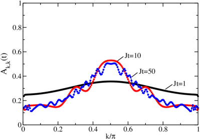
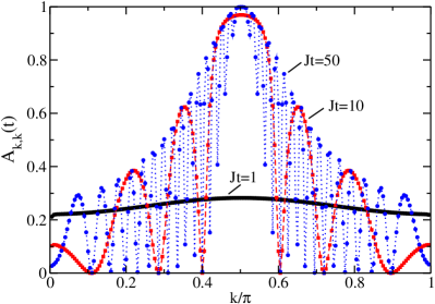
Figure 7: Diagonal part of the single-particle density matrix $A_{k,k}(t)$ for an inhomogeneous chain hopping, $\gamma_{l}=J\exp(-l/L)$, with $L=200$, for the Hermitian time evolution (left) and the ratchet case (right).

In the case of an inhomogeneous coupling, $\gamma_{l}=J\exp(-l/L)$, the single-particle density matrix is no longer diagonal. The solution of the equations (4.23) and (4.29) for $L=200$ sites shows that dephasing is very efficient for the non-diagonal elements $A_{k,p\neq k}$. Even at short times, $Jt\sim 1$, the single-particle density matrix is almost diagonal with $A_{k,p\neq k}(t)$ being an order of magnitude smaller than $A_{k,k}(t)$ for all $k,p$. Further decay in time of the off-diagonal elements is only algebraic thus leading to an algebraically decaying current density, see the following discussion. In Fig. 7 we show the time evolution of the diagonal components of the single-particle density matrix, $A_{k,k}(t)$. The qualitative behavior of $A_{k,k}(t)$ is the same for the homogenous and the inhomogeneous coupling. Note that the different chain fillings for the same parameter set lead to a different overall scale for $A_{k,k}$. The comparison shows that the frequency and the size of the beating oscillations is smaller in the Hermitian time evolution than in the ratchet case. For an inhomogeneous hybridization, $k$ is no longer a good quantum number. Apparently, the mode coupling in the Hermitian case noticeably reduces the fluctuations of $A_{k,k}(t)$ around its time average. In the ratchet case, the Hamiltonian can still be written as a sum over commuting $k$-modes, see eq. (4.24). Therefore, we observe a pronounced beating in $A_{k,k}(t)$ even for inhomogeneous hybridizations. As we shall see in Sect. 5, interactions introduce a strong scattering between particles so that oscillations of the $k$ modes are absent and $A_{k,k}(t)$ quickly relaxes to its steady-state distribution.

The non-diagonal components of $A_{k,p}$ enter the expression for the current density (3.6). A small transient current sets in at $t>0$ and decays to zero for long times $Jt\gg 1$. For our case study we choose $\gamma_{l}=J\exp(-l/L)$ so that we insert particles more readily in the left part of the chain than in the right. Originally, there is a current from the left to the right of the chain ($j_{c}>0$) which is reflected at the right chain end so that $j_{c}(t)$ changes sign as a function of time. As for the particle density, the current density shows oscillations which decay algebraically.

In Fig. 8 we show the transient current density for the Hermitian time evolution and the ratchet case for $L=200$ sites. The amplitudes differ for the same parameter set which is mostly due to the fact that there are more particles in the chain for the ratchet case. The frequency of the current oscillations is comparable. The current oscillations correspond to a swapping of the particles between the right and left chain boundaries. Since the mobile particles are concentrated around $\varepsilon(k_{0})=0$ ($k_{0}=\pi/2)$, their dominant velocity is given by $v_{0}=\left.(\partial\varepsilon(k))/(\partial k)\right|_{k=k_{0}}=2$. Therefore, their travel time between the chain boundaries is $T/2\approx L/v_{0}=L/2$ so that the oscillation period is $T\approx L$. As seen in Fig. 8, this rule applies better for the ratchet case where the distribution $A_{k,p}(t)$ is more peaked around $(k,p)=(\pi/2,\pi/2)$.

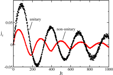
Figure 8: Current density $j_{c}(t)$ for non-interacting electrons for $\gamma_{l}=J\exp(-l/L)$, unitary and non-unitary time evolution, for $L=200$ sites.

4.2.2 Ratchet case

Here we derive the formulae on which the data in Figs. 6, 7 and 8 are based. Even in the case of a non-symmetric coupling we may write the ratchet Hamiltonian in the form

$$\hat{H}=\sum_{k=1}^{L}\hat{H}_{k}\quad,\quad\hat{H}_{k}=\varepsilon_{k}\hat{a}_{k}^{\dagger}\hat{a}_{k}+\hat{a}_{k}^{\dagger}\hat{B}_{k}$$ (4.24)

with $\left[\hat{H}_{k},\hat{H}_{p}\right]_{-}=0$ for all $k,p$. In eq. (4.24) we introduced the pseudo-fermionic operators

$$\hat{B}_{k}=\sqrt{\frac{2}{L+1}}\sum_{l=1}^{L}\gamma_{l}\sin\left(\frac{\pi kl}{L+1}\right)\hat{s}_{l}\;,$$ (4.25)

which obey $\left\{\hat{B}_{k},\hat{B}_{p}\right\}_{+}=\left\{\hat{B}_{k}^{\dagger},\hat{B}_{p}^{\dagger}\right\}_{+}=0$ for all $k,p$. In particular, $(\hat{B}_{k})^{2}=(\hat{B}_{k}^{\dagger})^{2}=0$. However, the operators and their adjoint do not anti-commute,

$$\left\{\hat{B}_{k},\hat{B}_{p}^{\dagger}\right\}_{+}=\frac{2}{L+1}\sum_{l=1}^{L}|\gamma_{l}|^{2}\sin\left(\frac{\pi kl}{L+1}\right)\sin\left(\frac{\pi pl}{L+1}\right)\equiv H(k,p)\;,$$ (4.26)

where we introduced the commutator function $H(k,p)$. For $\gamma_{l}=\gamma$, we have $\hat{B}_{k}=\gamma\hat{b}_{k}$ and $H(k,p)=|\gamma|^{2}\delta_{k,p}$.

The wave function can be obtained as in Sect. 4.2,

$$|\psi(t)\rangle=\prod_{k=1}^{L}\left(1+g_{k}(t)\hat{B}_{k}\hat{a}_{k}^{\dagger}\right)|\psi(0)\rangle\quad,\quad g_{k}(t)=\frac{1-e^{-{\rm i}\varepsilon_{k}t}}{\varepsilon_{k}}$$ (4.27)

because the components $\hat{H}_{k}$ of $\hat{H}$ commute with each other. As shown in appendix A, the single-particle density matrix can be written as

$$A_{p,q}=g_{q}g_{p}^{*}\left[H(p,q)+\sum_{k_{1},k_{2}=1}^{L}H(p,k_{1})\Sigma(k_{1},k_{2})H(k_{2},q)\right]\;,$$ (4.28)

where $\Sigma(k_{1},k_{2})$ are the entries of the self-energy matrix $\mathbf{\Sigma}$. This is obtained from the solution of the matrix equation

$$\mathbf{\Sigma}=-(\mathbf{1}+\mathbf{f}\cdot\mathbf{H})^{-1}\mathbf{f}\;.$$ (4.29)

Here, the entries of the matrices $\mathbf{1}$, $\mathbf{H}$ and $\mathbf{f}$ are $1_{a,b}=\delta_{a,b}$ (unit matrix), $H_{a,b}=H(a,b)$ (commutator matrix) and $f_{a,b}=\delta_{a,b}f_{a}$, $f_{a}=|g_{a}|^{2}$ (diagonal vertex matrix). The numerical solution requires the inversion of an $L\times L$ matrix.

5 Interacting fermions

In the thermodynamic limit and for non-interacting electrons, the average particle number in the chain goes to a constant at long-times only due to decoherence. On the other hand, a true relaxation of the particle density and other physical quantities can only take place when interactions are included.

To investigate the model with the density-density interaction terms, eq. (3.3), included, we use an adaptive time-dependent density matrix renormalization group ($t$-DMRG) algorithm. In DMRG the wave function of the problem under consideration is approximated by a matrix-product state in a truncated Hilbert space. The time evolution of this state is then calculated by using a second-order Trotter-Suzuki decomposition of the time-evolution operator. For details of the algorithm the reader is referred to Refs. [18, 19]. In our calculations we use a Trotter slicing $\delta t=0.1$ and keep $\chi=250$ states. It is known that the matrix dimension necessary to represent faithfully the time-evolved state increases exponentially with time. The $t$-DMRG algorithm is therefore only capable of describing the time evolution at short and intermediate times.

5.1 Particle number in the chain

In order to test the algorithm and the limitations for the time evolution, we perform numerical calculations for the particle density of non-interacting fermions with a homogeneous coupling where analytical results are available, see Sect. 4.1. In Fig. 9 we compare numerical results obtained with the $t$-DMRG algorithm with exact results in the non-interacting case, both for the unitary and ratchet time evolution. As seen from the figure, the $t$-DMRG results ($\chi=250$ states kept) are reliable for times $Jt\sim 14$ ($Jt\sim 8$) in the Hermitian (ratchet) time evolution.

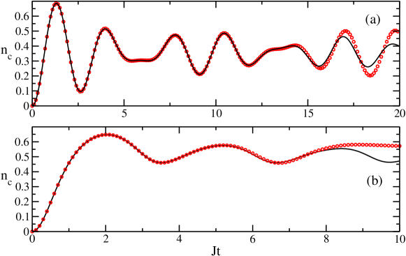
Figure 9: Particle density in the chain $n_{c}(t)$ for non-interacting fermions on a chain with $L=50$ sites (a) for the Hermitian time evolution ($\gamma/J=1$) and (b) for the ratchet time evolution ($\gamma_{\rm in}/J=1$). Full lines: analytical result; dots: data from $t$-DMRG ($\chi=250$ states kept).

Apparently, the $t$-DMRG is not able to reach the limit of large times when the two-level systems will have dephased completely. However, the algebraic decay of the phase coherence in $n_{c}(t)$ as given in eq. (4.13) and as shown in Fig. 2 is special to non-interacting fermions. Interactions between the particles lead to a much faster dephasing and, moreover, to a true relaxation.

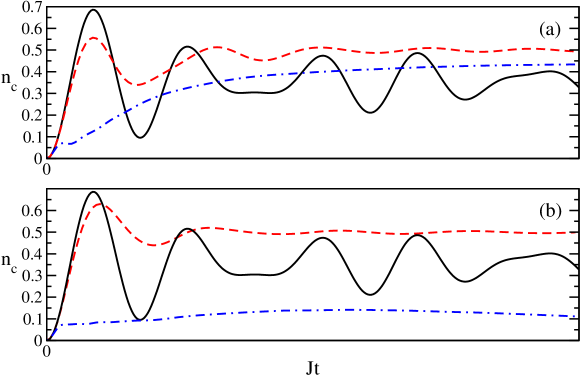
Figure 10: Particle density in the chain $n_{c}(t)$ for $L=50$ lattice sites and $\gamma/J=1$ for the Hermitian time evolution. We show $t$-DMRG results for non-interacting fermions ($V_{c}=V_{s}=V_{cs}=0$, solid lines) in comparison with interacting fermions: (a) $V_{c}=V_{cs}=2,V_{s}=0$ (dashed line) and $V_{c}=V_{cs}=8,V_{s}=0$ (dot-dashed line); (b) $V_{c}=V_{cs}=0,V_{s}=2$ (dashed line) and $V_{c}=V_{cs}=0,V_{s}=8$ (dot-dashed line).

In Fig. 10 we show examples for the particle density in the chain for the Hermitian time evolution ($\gamma/J=1$) in the presence of various types and strengths of the density-density interaction. In all cases, the interactions damp the oscillations and the average particle number reaches its limiting value much faster.

Depending on the type of interactions present, the energy of the system in its initial state

$$E_{\rm ini}=\langle\Psi_{0}|H|\Psi_{0}\rangle$$ (5.1)

is different. Since the Hamiltonian is a conserved quantity, the energy cannot change during time evolution. In the case where $V_{s}=0$ (Fig. 10a) the system starts in a state with $E_{\rm ini}=0$. Another state with zero potential energy for this type of density-density interactions is the twofold degenerate charge ordered state where chain and source sites are occupied alternatingly (Wigner lattice). This is shown pictorially in Fig. 11. At least in the limit where $V_{c}=V_{cs}$ is large, i.e., where the potential energy dominates over the kinetic energy, we therefore expect the system to reach a stationary state which is close to this charge ordered state. Therefore, the average particle density approaches $n_{c}(Jt\gg 1)=1/2$ (see Fig. 10a) for large interactions which is larger than in the non-interacting case. Apparently, the Coulomb interaction reduces the degree of delocalization of electrons on the chain whereby the Pauli blocking becomes less effective. The reduction of the Pauli pressure increases the density of fermions in the chain.

The case $V_{c}=V_{cs}=0$ with $V_{s}\neq 0$ (Fig. 10b) has an energy $E_{\rm ini}=(L-1)V_{s}$. For the situation where $V_{s}$ is smaller than the bandwidth, energy conservation can be fulfilled by compensating the loss of potential energy by kinetic energy which the fermions gain by entering the chain. Numerically we find that the density of these almost free fermions in the chain can reach $n_{c}(Jt\gg 1)\approx 1/2$, see Fig. 10b. For $V_{c}=V_{cs}=0$ with $V_{s}$ larger than the bandwidth, on the other hand, there is no possibility of compensating the loss in potential energy with kinetic energy in the chain. Hence the particles are almost all confined to the bath sites by energy conservation and $n_{c}(Jt\gg 1)$ remains small, see Fig. 10b.

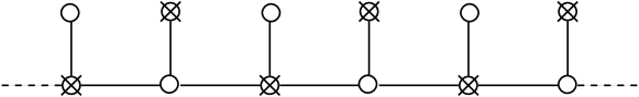
Figure 11: Charge ordering in a Wigner crystal state. The crosses mark the occupied sites.

The fast damping of the oscillations of the particle density is a genuine interaction effect which does not depend on the formation of a charge-density wave. This can be seen in Fig. 12 where we show the time evolution of the particle density in the chain for $V_{s}=V_{c}=V_{cs}=1,2,3,4$ and $\gamma=J=1$. As for $V_{c}=V_{cs}=0$, $V_{s}\neq 0$, due to the large initial energy, $E_{\rm ini}=(L-1)V_{s}$, of the system the number of accessible states is severely restricted. Therefore larger interactions, $V\geq 3$, not only lead to a faster relaxation but also suppress the particle density in the chain.

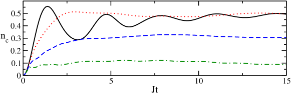
Figure 12: Particle density in the chain $n_{c}(t)$ for $L=50$ lattice sites and $\gamma/J=1$ for the Hermitian time evolution. We show $t$-DMRG results for interacting fermions: $V_{c}=V_{s}=V_{cs}=1$ (solid line), $V_{c}=V_{cs}=V_{s}=2$ (dotted line), $V_{c}=V_{cs}=V_{s}=3$ (dashed line), and $V_{c}=V_{cs}=V_{s}=4$ (dot-dashed line).

In the limit where $V_{s}=V_{c}=V_{cs}$ is much larger than the bandwidth, only the two states with the largest potential energies are reachable due to energy conservation: a full bath or a full chain. In general, the system can tunnel between these two possible states. For a large system size, however, the probability of all particles coherently tunneling is very small and therefore the associated timescale is very long. If we reduce the system size to $L=2$, on the other hand, the oscillations between these states occur on a relatively short timescale as can be seen in Fig. 13. For $L=2$ the Hamiltonian can be exactly diagonalized for arbitrary interactions and we show here exact results.

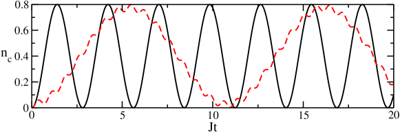
Figure 13: Particle density in the chain $n_{c}(t)$ for $L=2$ lattice sites and $\gamma/J=1$ for the Hermitian time evolution. We show exact results for non-interacting and interacting fermions: $V_{c}=V_{s}=V_{cs}=0$ (solid line), $V_{c}=V_{cs}=V_{s}=8$ (dashed line).

Next, we consider the ratchet case with interactions. Note that time evolution is limited to $Jt\leq 6$ so that we cannot follow the time evolution for too long. In Fig. 14 we show $t$-DMRG results for the ratchet case with $\gamma_{\rm in}/J=1$. Again, the interactions damp the fluctuations and, for the specific cases considered here. lead to an increase of the average particle number in the chain.

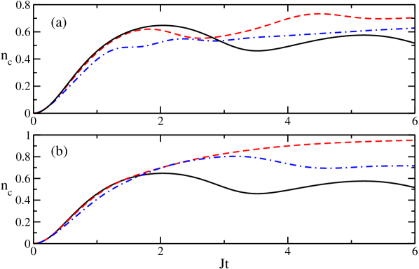
Figure 14: Particle density in the chain $n_{c}(t)$ for $L=50$ lattice sites and $\gamma_{\rm in}/J=1$ for the ratchet time evolution. We show $t$-DMRG results for non-interacting fermions ($V_{c}=V_{s}=V_{cs}=0$, solid lines) in comparison with interacting fermions; (a) $V_{c}=V_{cs}=2,V_{s}=0$ (dashed line) and $V_{c}=V_{cs}=4,V_{s}=0$ (dot-dashed line); (b) $V_{c}=V_{cs}=0,V_{s}=2$ (dashed line) and $V_{c}=V_{cs}=0,V_{s}=4$ (dot-dashed line).

5.2 Single-particle density matrix

We will concentrate on the Hermitian time evolution for which $t$-DMRG data are available for short and intermediate times. In the interacting case, scattering processes between fermions provide an efficient mechanism for the relaxation of the single-particle density matrix. Therefore, we expect that $A_{k,k}(Jt\gg 1)$ becomes independent of time. Note, however, that this distribution may, but need not, correspond to a thermal distribution for an appropriately chosen ensemble at a temperature determined by $\langle\hat{H}\rangle_{\textrm{thermal}}\equiv\langle\hat{H}\rangle_{\textrm{initial}}$. The interesting question whether or not this thermal state is reached will be addressed in a forthcoming publication [20].

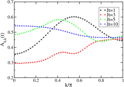
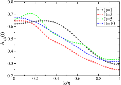
Figure 15: Single-particle density matrix $A_{k,k}(t)$ for the Hermitian time evolution with $\gamma/J=1$ for a chain of length $L=50$ with interaction parameters $V_{c}=V_{cs}=2$, $V_{s}=0$ (left) and $V_{c}=V_{cs}=0$, $V_{s}=2$ (right).

In Fig. 15 we show results for interaction parameters $V_{c}=V_{cs}=2$, $V_{s}=0$ and $V_{c}=V_{cs}=0$, $V_{s}=2$. For $V_{c}=V_{cs}=2$, $V_{s}=0$ at short times, the single-particle density matrix is still very close to the non-interacting case shown in Fig. 4. At longer times, the interactions lead to a rapid damping of the oscillations and, already at $Jt=10$, the distribution in both cases becomes almost time-independent. For $V_{c}=V_{cs}=2$, $V_{s}=0$ the distribution is very flat $A_{k,k}(t\gg 1)\simeq 1/2$. This observation supports our interpretation of the data shown in Fig. 10a: for strong interactions, the fermions tend to form a Wigner lattice of alternatingly occupied chain and source sites which corresponds to a completely flat single-particle density matrix. For $V_{c}=V_{cs}=0$, $V_{s}=2$, on the other hand, the distribution at long times resembles more a thermal Fermi distribution. Here the loss of potential energy due to particles leaving the bath has to be compensated by a gain in kinetic energy. For the interaction strength considered, approximately half of the particles enter the chain in the long-time limit, see Fig. 10b. These particles are almost free thus explaining why the long-time distribution shown in Fig. 15 is qualitatively similar to a thermalized free fermion distribution.

In contrast to the non-interacting case shown in Fig. 4, $A_{k,k}(t)$ is a smooth function of the pseudo-momentum $k$. Despite the fact that our $t$-DMRG cannot go much beyond $Jt=10$, our data suggest that the electron-electron interactions lead to a fast relaxation of the single-particle density matrix to its value in the long-time limit.

5.3 Current density

For non-interacting particles, the current decays to zero algebraically in time. The reason is the dephasing of the $k$-modes. In the presence of interactions, the current not only dephases but decays (exponentially) quickly. In Fig. 16 we show the result for the Hermitian time evolution for $L=50$ sites and two sets of interaction parameters. The fast decay of the current is clearly observed.

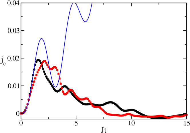
Figure 16: Current density $j_{c}(t)$ for interacting electrons for $\gamma_{l}=J\exp(-l/L)$ in the Hermitian time evolution ($J=1$) for $L=50$ sites with $V_{c}=V_{cs}=2,V_{s}=0$ (circles) and $V_{c}=V_{cs}=4,V_{s}=0$ (squares). For comparison we also show the result for noninteracting fermions (full line).

As discussed in Sect. 4.2, the inhomogeneous injection of non-interacting fermions results in a swapping of particles between the chain boundaries. As seen in Fig. 8, the current density increases to a maximal value of $j_{c,{\rm max}}^{\rm non-int}\approx 0.1$ at $Jt\approx 50$, oscillates with period $T\approx L$, and decays to zero algebraically slowly. For interacting fermions, however, the current density reaches its maximum of $j_{c,{\rm max}}^{\rm int}\approx 0.02$ at $Jt\approx 5$, and rapidly decays to very small values already at $Jt\approx 10$. Apparently, the interactions prevent the buildup of a coherent mesoscopic particle wave package, and only local transient current fluctuations can be seen. Note that this effect is most prominent in one dimension where particles can scatter forward and backward only. In addition, we have chosen quite sizable interactions to make the rapid relaxation visible within our restricted time interval in $t$-DMRG. For a more detailed analysis, longer times must be studied. This is beyond our numerical capabilities.

6 Summary and Conclusions

In this work, we studied the injection of spinless fermions from filled reservoir sites into an empty chain on which the particles can move between neighboring sites. We treated the cases of homogeneous and inhomogeneous hybridizations between the source and chain sites under a Hermitian time evolution and for the quantum ratchet case where the chain particles cannot return to the source sites. For non-interacting electrons, we provide analytical expressions as a function of time for the particle density, the single-particle density matrix, and the current density. In the presence of interactions, we use the $t$-DMRG algorithm to describe the time evolution of observables for short to medium time scales.

The Hermitian time evolution and the ratchet time evolution both show some qualitatively similar effects which is quite surprising at first. Despite the fact that the particles cannot return from the chain to the source sites in the ratchet case, their injection remains a coherent quantum-mechanical process. Therefore, the well-known quantum-mechanical phenomena such as constructive and destructive interference and Pauli blocking are seen in our observables. In particular, there are in both cases oscillations around the long-time average of the chain filling. Naturally, the results differ quantitatively. For example, the chain filling (transient current) is larger (smaller) for the ratchet case than for the Hermitian case for the same parameter set.

The time evolution of non-interacting particles is characterized by the absence of relaxation so that fairly large dephasing times, $Jt>10^{3}$, dominate the time evolution of our quantities. For large systems, the dephasing ultimately leads to steady-state expressions for the particle and current densities but the single-particle density matrix reveals that the spectrum is that of a single-particle Hamiltonian. For a homogeneous coupling, the system consists of independent two-level systems and the single-particle density matrix reflects the beating of these two-level systems. For inhomogeneous hybridizations, the beating of the diagonal terms $A_{k,k}(t)$ is less pronounced because $k$ is no longer a good quantum number. The inhomogeneous coupling between chain and source sites generates non-diagonal elements in the single-particle density matrix which, however, are small and dephase in time. They give rise to the coherent motion of a spreading particle wave packet between the chain ends which results in a transient oscillating current density.

When we introduce substantial interactions between the particles, the picture changes qualitatively. Depending on the type of density-density interactions considered, the system starts with different initial energies. Since the energy is conserved during time evolution, only parts of the Hilbert space are accessible. Interactions can therefore increase or decrease the particle density in the chain compared to the non-interacting case. Furthermore, the single-particle density matrix in the long-time limit can show a completely flat distribution in cases where the potential energy dominates, or become similar to a thermalized free fermion distribution when the kinetic energy plays the dominant role. Most importantly, instead of a slow dephasing or beating phenomena, we observe a rapid relaxation to stationary values on time scales $Jt=10$, not only for the particle and current densities but also for the single-particle density matrix. This shows the importance of interactions for a fast relaxation for all physical quantities of interest. In how far the obtained time-independent results do coincide with those predicted by thermodynamic considerations is a question we are planning to address in more detail elsewhere [20].

J.S. acknowledges support by the MAINZ (MATCOR) school of excellence and the DFG via the SFB/Transregio 49.

Appendix A Single-particle density matrix for non-interacting fermions (inhomogeneous ratchet case)

A.1 State

As seen from eq. (4.27), the time-dependent state is given by

$$|\psi(t)\rangle=\prod_{k=1}^{L}\left(1+g_{k}(t)\hat{B}_{k}\hat{a}_{k}^{\dagger}\right)|\psi(0)\rangle\;,$$ (A.1)

where $|\psi(0)\rangle=\prod\limits_{l=1}^{L}\hat{s}_{l}^{\dagger}|{\rm vac}\rangle$ and $g_{k}(t)=(1-e^{-{\rm i}\varepsilon_{k}t})/\varepsilon_{k}$. We rewrite the product as

$$|\psi(t)\rangle = \Bigl{[}1$$

$$+\sum_{k}g_{k}\hat{B}_{k}\hat{a}_{k}^{\dagger}$$

$$+\sum_{k_{1}<k_{2}}g_{k_{1}}g_{k_{2}}\hat{B}_{k_{1}}\hat{a}_{k_{1}}^{\dagger}\hat{B}_{k_{2}}\hat{a}_{k_{2}}^{\dagger}$$

$$+\sum_{k_{1}<k_{2}<k_{3}}g_{k_{1}}g_{k_{2}}g_{k3}\hat{B}_{k_{1}}\hat{a}_{k_{1}}^{\dagger}\hat{B}_{k_{2}}\hat{a}_{k_{2}}^{\dagger}\hat{B}_{k_{3}}\hat{a}_{k_{3}}^{\dagger}$$

$$+\dots\Bigr{]}|\psi(0)\rangle\;.$$

The first term, eq. (A.2), describes a state where there is no particle on the chain, the second term, eq. (A.2) describes the situation with one particle on the chain, and so on.

A.2 Numerator

In the density matrix $A_{p,q}$, the operator $\hat{a}_{p}^{\dagger}\hat{a}_{q}$ does not change the number of particles on the chain. Therefore,

$$\langle\psi(t)|\hat{a}_{p}^{\dagger}\hat{a}_{q}|\psi(t)\rangle = g_{q}g_{p}^{*}\langle\hat{B}_{p}^{\dagger}\hat{B}_{q}\rangle_{0}$$

$$+\sum_{k\neq(p,q)}\frac{g_{q}g_{k}}{2}\sum_{k_{1}\neq k_{2}}g_{k_{1}}^{*}g_{k_{2}}^{*}\langle\hat{a}_{k_{2}}\hat{B}_{k_{2}}^{\dagger}\hat{a}_{k_{1}}\hat{B}_{k_{1}}^{\dagger}\hat{B}_{k}\hat{a}_{k}^{\dagger}\hat{B}_{q}\hat{a}_{p}^{\dagger}\rangle_{0}$$

$$+\sum_{k_{1}<k_{2}\neq(q,p)}\frac{g_{q}g_{k_{1}}g_{k_{2}}}{6}\begin{array}[t]{@{}l@{}}\sum\limits_{\begin{subarray}{c}s_{1},s_{2},s_{3}\\ s_{1}\neq s_{2}\neq s_{3}\neq s_{1}\end{subarray}}g_{s_{1}}^{*}g_{s_{2}}^{*}g_{s_{3}}^{*}\\[18.0pt] \phantom{\sum_{A}^{B}}\times\langle\hat{a}_{s_{3}}\hat{B}_{s_{3}}^{\dagger}\hat{a}_{s_{2}}\hat{B}_{s_{2}}^{\dagger}\hat{a}_{s_{1}}\hat{B}_{s_{1}}^{\dagger}\hat{B}_{k_{1}}\hat{a}_{k_{1}}^{\dagger}\hat{B}_{k_{2}}\hat{a}_{k_{2}}^{\dagger}\hat{B}_{q}\hat{a}_{p}^{\dagger}\rangle_{0}\end{array}$$

$$+\dots\;.$$

We can factor out the expectation value for the chain operators and use Wick’s theorem [21] so that we can identify some of the momenta. Relabeling some indices leads to the following expressions for the second and third term of the numerator,

(A.3) $$= \sum_{k\neq(p,q)}g_{q}g_{k}g_{k}^{*}g_{p}^{*}\langle\hat{B}_{p}^{\dagger}\hat{B}_{k}^{\dagger}\hat{B}_{k}\hat{B}_{q}\rangle_{0}\;,$$ (A.4)

(A.3) $$= \sum_{\begin{subarray}{c}k_{1}<k_{2}\\ k_{1},k_{2}\neq(q,p)\end{subarray}}g_{q}g_{p}^{*}|g_{k_{1}}|^{2}|g_{k_{2}}|^{2}\langle\hat{B}_{p}^{\dagger}\hat{B}_{k_{2}}^{\dagger}\hat{B}_{k_{1}}^{\dagger}\hat{B}_{k_{1}}\hat{B}_{k_{2}}\hat{B}_{q}\rangle_{0}\;.$$ (A.5)

The expectation values are calculated using Wick’s theorem. To this end we need $\langle\hat{B}_{p}^{\dagger}\hat{B}_{q}\rangle_{0}=H(p,q)$, see eq. (4.26). The expectation values in eqs. (A.4) and (A.5) can be expressed as determinants,

$$\langle\hat{B}_{p}^{\dagger}\hat{B}_{k}^{\dagger}\hat{B}_{k}\hat{B}_{q}\rangle_{0} = \left|\begin{array}[]{cc}H(p,q)&H(p,k)\\ H(k,q)&H(k,k)\end{array}\right|$$ (A.8)

$$\langle\hat{B}_{p}^{\dagger}\hat{B}_{k_{2}}^{\dagger}\hat{B}_{k_{1}}^{\dagger}\hat{B}_{k_{1}}\hat{B}_{k_{2}}\hat{B}_{q}\rangle_{0} = \left|\begin{array}[]{ccc}H(p,q)&H(p,k_{1})&H(p,k_{2})\\ H(k_{1},q)&H(k_{1},k_{1})&H(k_{1},k_{2})\\ H(k_{2},q)&H(k_{2},k_{1})&H(k_{2},k_{2})\end{array}\right|\;.$$ (A.12)

This leads to the result

$$\langle\psi(t)|\hat{a}_{p}^{\dagger}\hat{a}_{q}|\psi(t)\rangle = g_{q}g_{p}^{*}\Biggl{[}H(p,q)+\sum_{k}|g_{k}|^{2}\left|\begin{array}[]{cc}H(p,q)&H(p,k)\\ H(k,q)&H(k,k)\end{array}\right|$$ (A.19)

$$+\frac{1}{2}\sum_{k_{1},k_{2}}|g_{k_{1}}|^{2}|g_{k_{2}}|^{2}\left|\begin{array}[]{ccc}H(p,q)&H(p,k_{1})&H(p,k_{2})\\ H(k_{1},q)&H(k_{1},k_{1})&H(k_{1},k_{2})\\ H(k_{2},q)&H(k_{2},k_{1})&H(k_{2},k_{2})\end{array}\right|+\ldots\Biggr{]}\;.$$

We were allowed to drop the restriction on the summations due to the properties of the determinants.

A.3 Self-energy

As in all perturbative calculations, we can translate the terms in (A.19) into diagrams [21] with ‘internal vertices’ $k$ of strength $f_{k}=|g_{k}|^{2}$ and lines between vertices $k_{1}$ and $k_{2}$ representing the factors $H(k_{1},k_{2})$. In the thermodynamic limit, $L\to\infty$, the linked-cluster theorem applies [21], i.e., the denominator $\langle\psi(t)|\psi(t)\rangle$ in $A_{p,q}$ cancels the unconnected diagrams in the numerator. In $A_{p,q}$ we have to sum over all diagrams which connect the external vertex $p$ with the external vertex $q$. We find

$$A_{p,q}=g_{q}g_{p}^{*}\left[H(p,q)-\sum_{k}H(p,k)f_{k}H(k,q)+\sum_{k_{1},k_{2}}H(p,k_{1})f_{k_{1}}H(k_{1},k_{2})f_{k_{2}}H(k_{2},q)\mp\ldots\right]\;.$$ (A.20)

We introduce the self-energy $\Sigma(a,b)$ [21] and prove eq. (4.28),

$$A_{p,q}=g_{q}g_{p}^{*}\left(H(p,q)+\sum_{k_{1},k_{2}}H(p,k_{1})\Sigma(k_{1},k_{2})H(k_{2},q)\right)\;,$$ (A.21)

where the self-energy entry $\Sigma(a,b)$ is obtained by summing all possible paths from the internal vertex $a$ to the internal vertex $b$ with altogether $n$ internal vertices ($n=1,2,\ldots$) and $(n-1)$ lines between them,

$$\Sigma(a,b) = -\delta_{a,b}f_{a}+f_{a}\Bigl{[}H(a,b)f_{b}-\sum_{k}H(a,k)f_{k}H(k,b)f_{b}$$ (A.22)

$$+\sum_{k_{1},k_{2}}H(a,k_{1})f_{k_{1}}H(k_{1},k_{2})f_{k_{2}}H(k_{2},b)f_{b}\mp\ldots\Bigr{]}$$

$$= -\delta_{a,b}f_{a}-f_{a}\sum_{k}H(a,k)\Sigma(k,b)\;.$$

The solution of this matrix equation provides $\mathbf{\Sigma}$, see eq. (4.29).

References

- [1] F. Gebhard and K. zu Münster, Ann. Phys. (Berlin) 523, 552 (2011).
- [2] T. Kinoshita, T. Wenger, and D. S. Weiss, Nature 440, 900 (2006).
- [3] S. Hofferberth, I. Lesanovsky, B. Fischer, T. Schumm, and J. Schmiedmayer, Nature 449, 324 (2007).
- [4] M. Rigol, V. Dunjko, and M. Olshanii, Nature 452, 854 (2008).
- [5] J. M. Deutsch, Phys. Rev. A 43, 2046 (1991).
- [6] M. Srednicki, Phys. Rev. E 50, 888 (1994).
- [7] T. Gericke, P. Wurtz, D. Reitz, T. Langen, and H. Ott, Nature 4, 949 (2008).
- [8] N. Strohmaier, D. Greif, R. Jördens, L. Tarruell, H. Moritz, T. Esslinger, R. Sensarma, D. Pekker, E. Altman, and E. Demler, Phys. Rev. Lett. 104, 080401 (2010).
- [9] P. Reimann, M. Grifoni, and P. Hänggi, Phys. Rev. Lett. 79, 10 (1997).
- [10] P. Hänggi, F. Marchesoni, and F. Nori, Ann. Phys. (Leipzig) 14, 51 (2005).
- [11] G. G. Carlo, G. Benenti, G. Casati, and D. L. Shepelyansky, Phys. Rev. Lett. 94, 164101 (2005).
- [12] N. Hatano and D. R. Nelson, Phys. Rev. Lett. 77, 570 (1996).
- [13] A. Mostafazadeh, J. of Math. Phys. 43, 205 (2002).
- [14] C. M. Bender and S. Boettcher, Phys. Rev. Lett. 80, 5243 (1998).
- [15] C. M. Bender, Rep. Prog. Phys. 70, 947 (2007).
- [16] A. Kossakowski, Rep. Math. Phys. 3, 247 (1972).
- [17] G. Lindblad, Commun. Math. Phys. 48, 119 (1976).
- [18] A. J. Daley, C. Kollath, U. Schollwöck, and G. Vidal, J. Stat. Mech. , P04005 (2004).
- [19] S. R. White and A. E. Feiguin, Phys. Rev. Lett. 93, 076401 (2004).
- [20] N. Sedlmayr, J. Ren, J. Sirker, and F. Gebhard (2011), in preparation.
- [21] A. L. Fetter and J. D. Walecka, Quantum Theory of Many-Particle Systems (McGraw-Hill, New York, 1980).