Fluctuation-induced traffic congestion in heterogeneous networks

Abstract

In studies of complex heterogeneous networks, particularly of the Internet, significant attention was paid to analyzing network failures caused by hardware faults or overload, where the network reaction was modeled as rerouting of traffic away from failed or congested elements. Here we model another type of the network reaction to congestion – a sharp reduction of the input traffic rate through congested routes which occurs on much shorter time scales. We consider the onset of congestion in the Internet where local mismatch between demand and capacity results in traffic losses and show that it can be described as a phase transition characterized by strong non-Gaussian loss fluctuations at a mesoscopic time scale. The fluctuations, caused by noise in input traffic, are exacerbated by the heterogeneous nature of the network manifested in a scale-free load distribution. They result in the network strongly overreacting to the first signs of congestion by significantly reducing input traffic along the communication paths where congestion is utterly negligible.

All Internet users are familiar with the feeling of frustration when their network connection slows down or halts. Barring cascading failures Watts (2002); Barrat et al. (2008); Motter and Lai (2002); *Motter:03; Moreno et al. (2003); Ashton et al. (2005); Wang and Kim (2007); Buldyrev et al. (2010); *Vespignani:10 which can shut down parts of the network, such a slowdown is a sign of network congestion which happens when the traffic load on some network elements exceeds their capacity Barrat et al. (2008); Motter and Lai (2002); *Motter:03; Moreno et al. (2003); Wang and Kim (2007). For the Internet congestion can be quantified as a relative difference between the rates of sent and delivered data packets Barrat et al. (2008); Arenas et al. (2001), with excess packets being eventually dropped. The first network reaction to a lost packet is a significant reduction of a transmission rate at the source followed by a slow recovery to the normal rate. When several loss events occur in quick succession, a multiplicative reduction drastically suppresses the transmission rate, which feels as congestion for the end user. If congestion persists for longer, the network eventually reroutes traffic away from congested links which may overload other links triggering a cascade of failures Moreno et al. (2003).

A surprising result of the considerations presented here is that transmission rates might be significantly reduced when the relative number of lost packets is utterly negligible. Such a reduction results from the existence of strong fluctuations of data losses along a typical communication path at the very onset of congestion. The loss fluctuations arise at each link at the threshold of its capacity due to noise in input traffic. Although such fluctuations exist only on shorter, mesoscopic time scales and will die out in time, we show that they might trigger an overreaction of a typical transport protocol to the first signs of losses. Normally the protocol aggressively reduces traffic rates along the routes perceived as congested due to multiple loss events. The overreaction results from the probability of such events on the mesoscopic scale being much higher than the product of the single-event probabilities.

The fluctuations are greatly magnified in heterogenous networks characterized by a power law (PL) distribution of the link load since congestion on links with high load affects a disproportionately large number of communication paths, as illustrated in Fig. 1. The link load in a network with a homogeneous traffic input distribution is proportional to the link betweenness $B_{i}$ (roughly, the number of shortest paths through link $i$) Freeman (1977); *Newman:01; *Newman:02. Many heterogeneous networks, including the Internet, fall into the category of scale-free (SF) networks characterized by the PL distribution of node degree Barabási and Albert (1999); Faloutsos et al. (1999); Pastor-Satorras et al. (2001); Albert and Barabási (2002); Pastor-Satorras and Vespignani (2004). Load distribution in SF networks also follows a (truncated) PL Pastor-Satorras and Vespignani (2004); Goh et al. (2001); *Goh:02; *Barthelemy:03; *Goh:03; Boccaletti et al. (2006); *Dorogovtsev:08,

$${\mathcal{P}}_{\mathrm{L}}(\ell) \propto\ell^{-2-\delta}\,,$$ (1)

with an almost universal exponent, $2+\delta\sim 2.0\div 2.3$. The load distribution of the real Internet was found Pastor-Satorras and Vespignani (2004); Vázquez et al. (2002); Dimitropoulos et al. (2005) to be in agreement with the above.

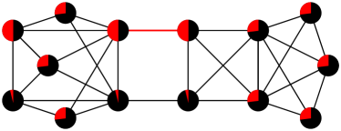
Figure 1: The importance of links with high betweenness (load): one congested link ($3\%$ of all the links here) affects $27\%$ of all the shortest paths. A light-shaded sector on each node indicates the fraction of congested paths originated on it.

We focus on a critical regime at the onset of congestion with a small imbalance, $\eta_{i}\equiv 1-\tau_{i}r_{i}$, between the average packet arrival rate (load), $1/\tau_{i}$, and departure rate (capacity), $r_{i}$, at link $i$. The nodes in the Internet core are routers and the links are output memory buffers (with attached transmission lines). For $\eta_{i}>0$ a memory buffer eventually becomes full and a newly arrived packet is dropped. On average, $\eta_{i}\!=\!\left\langle\Phi_{i}(T)\right\rangle$ where $\Phi_{i}(T)$ is the fraction of packets dropped during an observation time window $T$. Shifting this window in time causes $\Phi$ to fluctuate due to inevitable flow fluctuations de Menezes and Barabási (2004); *Meloni2008. We show the loss fluctuations to be crucial for network transport at certain mesoscopic time scale; for large enough $T$ they die out and $\Phi_{i}$ equals $\eta_{i}$. Positive $\eta_{i}$ plays the role of a local congestion parameter: their sum defines the network congestion parameter Barrat et al. (2008); Arenas et al. (2001).

Relative loss, $\Phi$, along a typical communication path is governed by losses in the comprising links and fluctuates due to both the noise in each link and a random choice of links in the path. The probability of a randomly picked link to be in the path is proportional to its betweenness. Hence, in a network with average link betweenness $\bar{B}$, a small loss along a path with $a$ links is given by

$${\Phi} =\sum_{i=1}^{a}{\ell}_{i}\Phi_{i}\,, {\ell}_{i} \equiv{B_{i}}/{\bar{B}}\,,$$ (2)

The quenched distribution of the relative load $\ell_{i}$ is given by the truncated PL (1), cut from below by $\ell\!\sim\!1$. The upper cutoff is irrelevant for $\delta>0$.

To describe noise in packet arrivals at link $i$ we assume, without loss of generality, that the inter-arrival time is random, with average $\tau_{i}$, while packets have a fixed length $l_{0}$. Arriving packets join the queue in the memory buffer. The queue length, $x_{i}({t})$ (measured in $l_{0}$), performs a random walk bounded by a buffer size $c_{i}$. The probability density, $w_{i}$, of diffusion from $x^{\prime}$ to $x$ over time $t$ obeys the Fokker-Planck equation with diffusion and advection coefficients $D_{i}\equiv 1/\tau_{i}$ and $V_{i}\equiv\eta_{i}/\tau_{i}$ and the probability-conservation boundary conditions:

$$\partial_{t}w_{i}(x,x^{\prime};t)=\left[{-V_{i}\partial_{x}+D_{i}\partial_{x}^{2}}\right]w_{i}(x,x^{\prime};t)\,.$$ (3)

In the critical regime the queue hovers at the boundary. A newly arriving packet is dropped every time when the queue length $x_{i}(t)$ overflows reaching the boundary layer, $c_{i}-1\leqslant x_{i}(t)\leqslant c_{i}$. Thus the fraction of packets lost over an observation time $T\!\gg\!\tau_{i}$ is

$$\Phi_{i}({T}) =\frac{1}{T}\int_{0}^{T}{\mathrm{d}}t\,\theta\left[x_{i}({t})-c_{i}+1\right]=\frac{1}{K_{i}}\sum_{k=1}^{K_{i}}\delta_{k}\,,$$ (4)

where $K_{i}\equiv\left[{T}/{\tau_{i}}\right]\gg 1$ is the number of packets arrived over time $T$, and $\delta_{k}$ equals $1$ if $x_{i}({t})$ reached the boundary layer at the $k^{\mathrm{th}}$ step, or $0$ otherwise.

To find the probability density function (PDF) of $\Phi_{i}$, we begin with the characteristic function, $\chi_{T}(q_{i})=\langle\mathrm{e}^{\mathrm{i}q_{i}\Lambda_{i}}\rangle\,$, of the distribution of a cumulative loss, $\Lambda_{i}\!=\!(T/\tau_{i})\Phi_{i}(T)$. Using Eqs. (3) and (4) we represent $\chi_{T}$ as the sum of time-ordered integrals

$$\chi_{T}(q_{i})=\sum_{n=0}^{\infty}({{\mathrm{i}q_{i}}})^{n}\!\!\int\!\mathrm{d}^{n}t\,{\mathcal{R}}_{i}({t_{n}\!-\!t_{n-1}})\dots\mathcal{R}_{i}({t_{2}\!-\!t_{1}})p_{i}\,,$$

running over the regions $0<t_{1}<\dots<t_{n}<T$. Here $p_{i}\equiv w_{i}({c_{i},x^{\prime};t\to\infty})=\eta_{i}\left(1-\mathrm{e}^{-\eta_{i}c_{i}}\right)^{-1}$ is the stationary probability density for the queue to be in the boundary layer and ${\mathcal{R}}_{i}(t)=w({c_{i},c_{i};t})$ is the return probability. We rewrite the expression for $\chi_{T}$ as the integral equation

$${\chi}_{T}(q_{i})\!-\!1={\mathrm{i}}q_{i}\biggl{\{}p_{i}T+\!\!\int_{0}^{T}\!\!\mathrm{d}t\,{\mathcal{R}_{i}}(T\!-\!t)\,\left[{\chi}_{t}(q_{i})-1\right]\!\biggr{\}}.$$ (5)

The inverse Fourier transform from $q_{i}$ to $\Lambda_{i}$ shows the PDF of $\Lambda_{i}$ to be the sum $\mathcal{F}_{T}({\Lambda_{i}})+A_{i}\delta({\Lambda_{i}})$, with $\mathcal{F}$ describing losses ($\Lambda_{i}>0$) and $A_{i}$ the probability of no losses over the time $T$, with $1=A_{i}+\int_{0}^{\infty}\!\mathrm{d}\Lambda\ {\mathcal{F}}_{T}(\Lambda)$. Solving Eq. (5) by the Laplace transform with respect to $T$ gives

$${\mathcal{F}}_{\varepsilon}(\Lambda_{i}) =\frac{p_{i}\mathrm{e}^{-\frac{\Lambda_{i}}{\mathcal{R}_{\,\varepsilon}}}}{\tau_{i}\varepsilon^{2}\,\mathcal{R}_{\,\varepsilon}^{2}}\,, \mathcal{R}_{\,\varepsilon} =\frac{\sqrt{\eta_{i}^{2}+4\tau_{i}{\varepsilon}}+{\eta_{i}}}{2\tau_{i}\varepsilon}\,.$$ (6)

For a perfectly designed network with fully utilized resources for homogeneous input traffic, $c_{i}$ and $\tau_{i}^{-1}$ are proportional to the relative link load Goh et al. (2001), $c_{i}\equiv c{\ell}_{i}$ and $\tau_{i}^{-1}\equiv{\ell}_{i}\tau^{-1}$, while the imbalance $\eta_{i}$ is $\ell_{i}$-independent. Then the congestion threshold $\eta_{i}=0$ is reached simultaneously by all links. Naturally, such a complete utilization is impossible: design imperfections and local variations of demand cause the congestion thresholds to spread Wang and Kim (2007). We model such a spread (quenched on the relevant time scales) as a sharply peaked symmetric distribution of $\eta_{i}$ with criticality width $\gamma\ll 1$. Realistic regimes are bounded by $a\ll\gamma^{-1}\lesssim c$, as for $\gamma^{-1}\gtrsim c$ congestion thresholds are still reached simultaneously, while a network with $a\gamma\gtrsim 1$ would be permanently congested.

The PDF of $\Phi_{i}$ has the same form as that of $\Lambda_{i}$, namely $A_{i}\delta({\Phi_{i}})+{P}_{T}(\Phi_{i};\ell_{i})$, where its lossy part, ${P}_{T}(\Phi_{i};\ell_{i})$, is found for fixed $\ell_{i}$ and $\eta_{i}$ by rescaling $\mathcal{F}_{T}$, the inverse Laplace transform of Eq. (6), as $(\ell_{i}/\varphi_{0}^{2}){\mathcal{F}}_{T}\!\left(\ell_{i}\Phi_{i}/\varphi_{0}^{2}\right)$. The averaging over $\eta$ is straightforward and preserves very different shapes of $P_{T}$ on the mesoscopic time scale, $\ell_{i}\gamma^{2}\!\ll\!\tau/T\!\equiv\!\varphi_{0}^{2}\!\ll\!\gamma$, and macroscopic one, $\varphi_{0}^{2}\!\ll\!\gamma$. In the former case, the congestion spread is so narrow that to average over it one replaces $\eta_{i}$ by $\gamma$ which gives the averaged PDF $\sim\ell_{i}\gamma/\varphi_{0}^{2}$ for $0<\Phi_{i}\lesssim\varphi_{0}/\sqrt{\ell_{i}}$ followed by a decay $\sim\mathrm{e}^{-\Phi_{i}^{2}\ell_{i}/\varphi_{0}^{2}}$ for bigger $\Phi_{i}$. The probability of loosing a packet, $1-A_{i}\sim\gamma\sqrt{\ell_{i}}/\varphi_{0}\ll 1$, is small. For macroscopic times, the Laplace transform in Eq. (6) is exponential, corresponding to the averaged PDF given by $\delta({\Phi_{i}-\eta_{i}})$ for $\eta_{i}>0$ : on this scale ${P}_{T}(\Phi_{i};\ell_{i})$ repeats the shape of the criticality spread for positive $\eta_{i}$, while free-flow (lossless) links with negative $\eta_{i}$ give $A_{i}=\frac{1}{2}$.

The PDF of losses along path (2) is a convolution of PDFs of statistically independent ${\ell}_{i}\Phi_{i}$, averaged over the load distribution (1). It still has the structure $A\delta({\Phi})+P_{T}({\Phi})$ with $A=\prod_{i=1}^{a}\left\langle A_{i}\right\rangle_{\ell}$. For $\varphi_{0}\ll\gamma$ losses in each link in (2) are on the macroscopic time scale, light-shaded (green online) in Fig. 2. Then $A=2^{-a}\ll 1$ for $a\gg 1$ and, by the law of large numbers, $P_{T}({\Phi})$ is a normal distribution with average $\left\langle\Phi\right\rangle_{\mathrm{c}}\sim a\gamma\ll 1$ (where $\left\langle\dots\right\rangle_{\mathrm{c}}$ stands for the averaging over all the three sources of randomness) and width $\sim\left\langle\Phi\right\rangle_{\mathrm{c}}/\sqrt{a}$ (inset in Fig. 3).

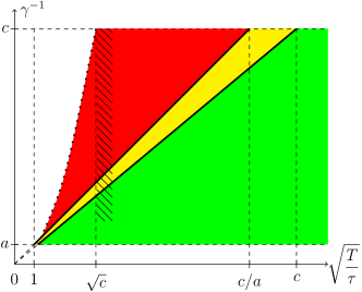
Figure 2: Different loss modes depending on the operation time $T$ and criticality width $\gamma$. The dark-shaded (red online) area above the upper bold line, $\gamma^{-1}=a\sqrt{T/\tau}$, represents the fluctuation-driven mesoscopic mode; the light-shaded (green online) area below the lower bold line, $\gamma^{-1}=\sqrt{T/\tau}$, the self-averaging macroscopic mode (microscopic times on the left of the parabola, $\gamma^{-1}=T/\tau$, are not considered). The crossover sector between the bold lines is narrow as $c\gg a\gg 1$ ($a$ is the number of links in path (2), $c$ is the memory buffer size for link with $\ell_{i}=1$). The hatched area shows the region of network feedback operations at the congestion onset.

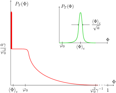
Figure 3: Probability distribution function, $P_{T}({\Phi})$, of relative losses in the critical regime at the onset of congestion. The average, $\left\langle\Phi\right\rangle_{\mathrm{c}}\sim a\gamma\ll 1$, is time-independent. The main figure shows (not to scale) $P_{T}({\Phi})$ when the observation time $T$ is on the mesoscopic scale. With increasing $T$, as $\varphi_{0}\!\equiv\!\sqrt{\tau/T}$ is moving towards $\left\langle\Phi\right\rangle_{\mathrm{c}}$, the plateau becomes narrower and higher, the tail squeezes, and the area of the peak at $\Phi=0$ shrinks. After passing through the intermediate time scale, $\langle{\varphi_{0}}\rangle$ becomes larger than $\left\langle\Phi\right\rangle_{\mathrm{c}}$ on the macroscopic time scale, where the PDF becomes Gaussian as shown in the inset.

The communication path is in a nontrivial fluctuation-driven mode only if all the comprising links are in that mode, obeying $\ell_{i}\ll\varphi_{0}^{2}/\gamma^{2}$. For $\delta>0$ in Eq. (1) and $a\gamma\!\ll\!\varphi_{0}\!\ll\!\sqrt{\gamma}$, which defines the mesoscopic time scale for the path shown as the dark-shaded area (red online) in Fig. 2, one has $A=\left({1-\gamma/\varphi_{0}}\right)^{a}\approx 1-a\gamma/\varphi_{0}$. The PDF has a peak at $\Phi\!=\!0$, describing the close-to-$1$ probability $A$ of not loosing a packet, while the lossy part, $P_{T}({\Phi})$, is dominated by (any) one link along the path: $P_{T}({\Phi})\cong a\left\langle{{\ell}^{-1}P_{T}(\Phi/{\ell};\ell)}\right\rangle_{\ell}$. The plateau in this rescaled PDF is stretched up to $\varphi_{0}\ell^{1/2}$ with height $a\gamma/\varphi_{0}^{2}$. For $\Phi\lesssim\varphi_{0}$ averaging over the distribution (1) leaves the plateau intact. For $\Phi\gtrsim\varphi_{0}$ the plateau exists only for links with load ${\ell}\gtrsim({\Phi/\varphi_{0}})^{2}$ which becomes the lower limit in the averaging over load. When the lower limit is much smaller than the upper, $({\varphi_{0}/\gamma})^{2}$, the averaging is contributed only by the former resulting in the PL tail

$$P_{T}(\Phi) \sim\frac{a\gamma}{\varphi_{0}^{2}}\left(\frac{\Phi}{\varphi_{0}}\right)^{-2(1+\delta)}\!\!\!, {\varphi_{0}}\lesssim{\Phi}\ll\frac{\varphi_{0}^{2}}{\gamma}\,,$$ (7)

followed by an exponentially small decay.

The entire PDF is shown in Fig. 3. The probability of losses is small but when losses do occur – the conditional probability of higher-than-average losses (governed by the long plateau and even longer heavy tail) is high: the losses are intermittent. The tail (7) is proportional to $a$ since it is dominated by losses in any one link along the path. On the other hand, this link is shared by a large number of paths as illustrated in Fig. 1.

The tail (7) is irrelevant for $\left\langle\Phi\right\rangle_{\mathrm{c}}$ if $\delta>0$ but dominates higher moments of intermittent losses if $\delta<\frac{1}{2}$. Remarkably, in the SF models of the Internet as well as in direct measurements of its link load Goh et al. (2001, 2002); Vázquez et al. (2002); Boccaletti et al. (2006); Dorogovtsev et al. (2008); Dimitropoulos et al. (2005) the exponent $2+\delta$ in Eq. (1) lies between $2.0$ and $2.3$, i.e. obeying $0<\delta<\frac{1}{2}$. The relative values of all higher moments in this mode are large: e.g., $\sqrt{\langle{\Phi^{2}}\rangle_{\mathrm{c}}}/\langle{\Phi}\rangle_{\mathrm{c}}\sim a^{1/2-\delta}(\varphi_{0}/a\gamma)^{1-\delta}\gg 1$.

This relatively high magnitude of higher moments means that losses occur in groups (intermittency). Indeed, the fraction of dropped pairs can be represented using Eq. (4) as $\frac{2}{K(K-1)}\sum_{k<j}\delta_{k}\delta_{j}$. It is approximately equal to $\Phi_{i}^{2}({T})$ if a typical number of lost packets, $\eta_{i}K_{i}$, is large. Similarly, the fraction of $n$-tuples of dropped packets is equal to $\Phi_{i}^{n}(T)$ (for $n\ll\eta_{i}K_{i}$). Then the small probability of loosing, e.g., three packets scale, $\left\langle\Phi^{3}\right\rangle_{\mathrm{c}}$, is much bigger on the mesoscopic time than the probability of three independent loss events, $\left\langle\Phi\right\rangle_{\mathrm{c}}^{3}$.

The intermittency is the reason of a strong adverse effect of the fluctuations on network feedback. We illustrate this for the feedback mechanism provided by an idealized transmission control protocol (TCP) which handles most of data transfer. It works in cycles, each consisting of sending a group of $W$ packets from the source and receiving acknowledgments of their delivery at the destination Kurose and Ross (2010). The transmission rate equals $W/t_{0}$ where the cycle duration $t_{0}$ is normally the round trip time. On establishing a connection, $W$ linearly increases in time until it reaches a steady-state value determined, in the absence of losses, by the end-user resources. If a loss is detected during the cycle, the protocol halves $W$. If losses occur in a few nearby cycles, $W$ is multiplicatively reduced. As it can increase only additively, such a multiple-loss event results in delays noticeable to the end user. Indeed, at the onset of congestion a typical round trip time is governed by a queue in a single full buffer Kurose and Ross (2010) and is of order $t_{0}=0.25$s. As in free-flow regime $W\gtrsim 100$, the time of resuming normal rate of service could be tens of seconds.

Hence, it is crucial to know whether the protocol operation time scale at the onset of congestion, $\varphi_{0}^{2}(t_{0})\!\equiv\!\tau/t_{0}$, falls into the mesoscopic mode where the relative probability of multiple losses is high. To this end note that the memory buffer size $c_{i}$ of any link is related to its capacity (maximal sending rate) $r_{i}$ by the engineering ‘rule of thumb’ Kurose and Ross (2010), $c_{i}=t_{0}r_{i}$, ensuring any full buffer to empty during the same time $t_{0}$. As $\tau_{i}r_{i}\lesssim 1$ at the congestion threshold, we find $\varphi_{0}^{2}(t_{0})\gtrsim 1/c$. We show this region of protocol operations as the hatched area in Fig. 2 which spreads by many orders in magnitude over $\gamma^{-1}$.

The criticality width $\gamma$ is not directly measurable but is bounded. The upper bound in Fig. 2, $\gamma^{-1}\lesssim c$, is approaching the perfect design (full utilization), as explained after Eq. (6). The lower bound, $\gamma^{-1}\gg aW$, is determined by the condition $\left\langle\Phi\right\rangle_{\mathrm{c}}\sim a\gamma\ll 1/W$: if it were not fulfilled, at least one packet per cycle would be lost resulting in a sharp reduction of the transmission rate after a few cycles, i.e. strong congestion. Assuming $c\sim 10^{6}$ for the typical buffer size (in packets) Kurose and Ross (2010), and $a\sim 10$ for the average number of links in an end-to-end path across the Internet, Albert and Barabási (2002); Barrat et al. (2008) we see that $aW$ is close to $\sqrt{c}$, so that almost the entire hatched area corresponds to the mesoscopic mode of intermittent losses.

On the macroscopic time scale (at the bottom of the hatched area) the probability $\left\langle\Phi^{2}\right\rangle_{\mathrm{c}}$ of detecting two loss indicators in two consecutive cycles is simply equal to $\left\langle\Phi\right\rangle_{\mathrm{c}}^{2}$. However, for larger $\gamma^{-1}$ the ratio ${\langle{\Phi^{2}}\rangle_{\mathrm{c}}}/\langle{\Phi}\rangle_{\mathrm{c}}^{2}$ increases reaching $c^{1-\delta}/a$ at the top, where $\gamma\sim c^{-1}$. There it varies from $10^{2}$ for $\delta=\frac{1}{2}$ to $10^{5}$ for $\delta\to 0$. Such a ratio for detecting three loss indicators in three consecutive cycles is even more striking, varying from $10^{6}$ to $10^{9}$. Conversely, the same multiple-loss indicators may correspond to very different average losses $a\gamma$. And it is the time-independent average loss which matters since the intermittent fluctuations would die out with time as operations move from the dangerous dark-shaded (red online) area to the safe light-shaded (green online) one, see Fig. 2. Hence, it is of great importance to design protocols capable of avoiding the overestimation of nascent losses by identifying in which loss mode the network operates and adjusting accordingly. To this end one needs to distinguish between single and multiple packet loss events within one cycle – the information which is not collected in normal TCP operations.

The key features of our model might be characteristic of complex networks other than the Internet. First, if link (or node) operations in a network can be described by a finite-capacity model, it will suffer from local congestion fluctuations at the threshold of capacity due to inevitable input noise. Secondly, if such a network is heterogeneous, with a PL load distribution, the fluctuations would be greatly enhanced on highly-loaded network elements. Finally, the fluctuations become really dangerous when they are misinterpreted by a network feedback mechanism – the transmission control protocol in the case of the Internet. This mechanism is specific for different types of network and whether it may trigger fluctuation-induced congestion requires ad hoc considerations.

This work was supported by the EPSRC Grant No. EP/E049095/1.

References

- Watts (2002) D. J. Watts, Proc. Natl. Acad. Sci. U.S.A. 99, 5766 (2002).
- Barrat et al. (2008) A. Barrat, M. Barthélemy, and A. Vespignani, Dynamic processes on complex networks (Cambridge Univ. Press, 2008).
- Motter and Lai (2002) A. E. Motter and Y.-C. Lai, Phys. Rev. E 66, 065102 (2002).
- Motter (2004) A. E. Motter, Phys. Rev. Lett. 93, 098701 (2004).
- Moreno et al. (2003) Y. Moreno, R. Pastor-Satorras, A. Vázquez, and A. Vespignani, Europhys. Lett. 62, 292 298 (2003).
- Ashton et al. (2005) D. J. Ashton, T. C. Jarrett, and N. F. Johnson, Phys. Rev. Lett. 94, 058701 (2005).
- Wang and Kim (2007) B. Wang and B. J. Kim, Europhys. Lett. 78, 48001 (2007).
- Buldyrev et al. (2010) S. V. Buldyrev, R. Parshani, G. Paul, H. E. Stanley, and S. Havlin, Nature 464, 1025 (2010).
- Vespignani (2010) A. Vespignani, Nature 464, 984 (2010).
- Arenas et al. (2001) A. Arenas, A. Díaz-Guilera, and R. Guimerà, Phys. Rev. Lett. 86, 3196 (2001).
- Freeman (1977) L. Freeman, Sociometry 40, 35 (1977).
- Newman (2001) M. E. J. Newman, Phys. Rev. E 64, 016132 (2001).
- Girvan and Newman (2002) M. Girvan and M. Newman, Proc. Natl. Acad. Sci. USA 99, 7821 7826 (2002).
- Barabási and Albert (1999) A.-L. Barabási and R. Albert, Science 286, 509 (1999).
- Faloutsos et al. (1999) M. Faloutsos, P. Faloutsos, and C. Faloutsos, Comp. Com. Rev. 29, 251 (1999).
- Pastor-Satorras et al. (2001) R. Pastor-Satorras, A. Vázquez, and A. Vespignani, Phys. Rev. Lett. 87, 258701 (2001).
- Albert and Barabási (2002) R. Albert and A.-L. Barabási, Rev. Mod. Phys. 74, 47 (2002).
- Pastor-Satorras and Vespignani (2004) R. Pastor-Satorras and A. Vespignani, Evolution and structure of the Internet (Cambridge Univ. Press, 2004).
- Goh et al. (2001) K. I. Goh, B. Kahng, and D. Kim, Phys. Rev. Lett. 87, 278701 (2001).
- Goh et al. (2002) K. I. Goh, E. Oh, H. Jeong, B. Kahng, and D. Kim, Proc. Natl. Acad. Sci. U.S.A. 99, 12583 (2002).
- Barthélemy (2003) M. Barthélemy, Phys. Rev. Lett. 91, 189803 (2003).
- Goh et al. (2003) K. I. Goh, C. M. Ghim, B. Kahng, and D. Kim, Phys. Rev. Lett. 91, 189804 (2003).
- Boccaletti et al. (2006) S. Boccaletti, V. Latora, Y. Moreno, M. Chavez, and D. U. Hwang, Phys. Rep. 424, 175 (2006).
- Dorogovtsev et al. (2008) S. N. Dorogovtsev, A. V. Goltsev, and J. F. F. Mendes, Rev. Mod. Phys. 80, 1275 (2008).
- Vázquez et al. (2002) A. Vázquez, R. Pastor-Satorras, and A. Vespignani, Phys. Rev. E 65, 066130 (2002).
- Dimitropoulos et al. (2005) X. A. Dimitropoulos, D. V. Krioukov, and G. F. Riley, “Revisiting internet AS-level topology discovery,” in Lect. Notes Comput. Sci. 3431, Vol. 3431, edited by C. Dovrolis (Springer, 2005) pp. 177–188.
- de Menezes and Barabási (2004) M. A. de Menezes and A.-L. Barabási, Phys. Rev. Lett. 92, 028701 (2004).
- Meloni et al. (2008) S. Meloni, J. Gómez-Gardeñes, V. Latora, and Y. Moreno, Phys. Rev. Lett. 100, 208701 (2008).
- Note (1) More accurate calculations show that the -function is smeared but the resulting width is much smaller than .
- Kurose and Ross (2010) J. F. Kurose and K. W. Ross, Computer networking : a top-down approach, 5th ed. (Addison Wesley, 2010).