General high-order rogue waves and their dynamics in the nonlinear Schrödinger equation

Abstract: General high-order rogue waves in the nonlinear Schrödinger equation are derived by the bilinear method. These rogue waves are given in terms of determinants whose matrix elements have simple algebraic expressions. It is shown that the general $N$-th order rogue waves contain $N-1$ free irreducible complex parameters. In addition, the specific rogue waves obtained by Akhmediev et al. (Phys. Rev. E 80, 026601 (2009)) correspond to special choices of these free parameters, and they have the highest peak amplitudes among all rogue waves of the same order. If other values of these free parameters are taken, however, these general rogue waves can exhibit other solution dynamics such as arrays of fundamental rogue waves arising at different times and spatial positions and forming interesting patterns.

1 Introduction

Rogue waves, also known as freak waves, monster waves, killer waves, extreme waves, and abnormal waves, is a hot topic in physics these days. This name comes originally from oceanography, and it refers to large and spontaneous ocean surface waves that occur in the sea and are a threat even to large ships and ocean liners. Recently, an optical analogue of rogue waves — optical rogue waves, was observed in optical fibres [2, 3]. These optical rogue waves are narrow pulses which emerge from initially weakly modulated continuous-wave signals. A growing consensus is that both oceanic and optical rogue waves appear as a result of modulation instability of monochromatic nonlinear waves. Mathematically, the simplest and most universal model for the description of modulation instability and subsequent nonlinear evolution of quasi-monochromatic waves is the focusing nonlinear Schrödinger (NLS) equation [4, 5, 6]. This equation is integrable [7], thus its solutions often admit analytical expressions. For rogue waves, the simplest (lowest-order) analytical solution was obtained by Peregrine [8]. This solution approaches a non-zero constant background as time goes to $\pm\infty$ but rises to a peak amplitude of three times the background in the intermediate time. Special higher-order rogue waves were obtained by Akhmediev, et al. using Darboux transformation [9]. These rogue waves could reach higher peak amplitude from a constant background. Recently, more general higher-order (multi-Peregrine) rogue waves were obtained by Dubard, et al. [10, 11] and Gaillard [12]. It was shown that these higher-order waves could possess multiple intensity peaks at different points of the space-time plane. These exact rogue-wave solutions, which sit on non-zero constant background, are very different from the familiar soliton and multi-soliton solutions which sit on the zero background. These rogue waves are intimately related to homoclinic solutions [13]. Indeed, rogue waves can be obtained from homoclinic solutions when the spatial period of homoclinic solutions goes to infinity [14]. These rogue waves are also related to breather solutions which move on a non-zero constant background with profiles changing with time [15].

In this article, we derive general high-order rogue waves in the nonlinear Schrödinger equation and explore their new solution dynamics. Our derivation is based on the bilinear method in the soliton theory [16]. Our solution is given in terms of Gram determinants and then further simplified so that the elements in the determinant matrices have simple algebraic expressions. Compared to the high-order rogue waves presented in [10, 12], our solution appears to be more explicit and more easily yielding specific expressions for rogue waves of any given order. We also show that these general rogue waves of $N$-th order contain $N-1$ free irreducible complex parameters. In addition, the specific rogue waves obtained in [9] correspond to special choices of these free parameters, and they have the highest peak amplitudes among all rogue waves of the same order. If other values of these free parameters are taken, however, these general rogue waves can exhibit other solution dynamics such as arrays of fundamental (Peregrine) rogue waves arising at different times and spatial positions. Interesting patterns of these rogue-wave arrays are also illustrated.

2 General rogue-wave solutions

In this article, we consider general rogue waves in the focusing NLS equation

$$iu_{t}=u_{xx}+2|u|^{2}u.$$ (1)

Rogue waves are nonlinear waves which approach a constant background at large time and distances. Notice that Eq. (1) is invariant under scalings $x\to\alpha x$, $t\to\alpha^{2}t$, $u\to u/\alpha$ for any real constant $\alpha$. In addition, it is invariant under the Galilean transformation $u(x,t)\to u(x-vt,t)\mbox{exp}(-ivx/2+iv^{2}t/4)$ for any real velocity $v$. Thus we only consider rogue waves which approach unit-amplitude background at large $x$ and $t$,

$$u(x,t)\to e^{-2it},\quad x,t\to\pm\infty.$$

Then under the variable transform $u\to ue^{-2it}$, the NLS equation (1) becomes

$$iu_{t}=u_{xx}+2(|u|^{2}-1)u,$$ (2)

where

$$u(x,t)\to 1,\quad x,t\to\pm\infty.$$ (3)

The rogue waves are described by rational solutions in the NLS equation. In order to present these solutions, let us introduce the so-called elementary Schur polynomials $S_{n}(\mbox{\boldmath$x$})$ which are defined via the generating function,

$$\sum_{n=0}^{\infty}S_{n}(\mbox{\boldmath$x$})\lambda^{n}=\exp\left(\sum_{k=1}^{\infty}x_{k}\lambda^{k}\right),$$

where $\mbox{\boldmath$x$}=(x_{1},x_{2},\cdots)$. For example we have

$$S_{0}(\mbox{\boldmath$x$})=1,\quad S_{1}(\mbox{\boldmath$x$})=x_{1},\quad S_{2}(\mbox{\boldmath$x$})=\frac{1}{2}x_{1}^{2}+x_{2},\quad S_{3}(\mbox{\boldmath$x$})=\frac{1}{6}x_{1}^{3}+x_{1}x_{2}+x_{3},\quad\cdots.$$

It is known that the general Schur polynomials give the complete set of homogeneous-weight algebraic solutions for the Kadomtsev-Petviashvili (KP) hierarchy [17, 18].

Theorem 1. The NLS equation (2) under the boundary condition (3) has nonsingular rational solutions

$$u=\frac{\sigma_{1}}{\sigma_{0}},$$ (4)

where

$$\sigma_{n}=\det_{1\leq i,j\leq N}\left(m_{2i-1,2j-1}^{(n)}\right),$$ (5)

the matrix elements in $\sigma_{n}$ are defined by

$$m_{ij}^{(n)}=\sum_{\nu=0}^{\min(i,j)}\Phi_{i\nu}^{(n)}\Psi_{j\nu}^{(n)},\quad\Phi_{i\nu}^{(n)}=\frac{1}{2^{\nu}}\sum_{k=0}^{i-\nu}a_{k}S_{i-\nu-k}(\mbox{\boldmath$x$}^{+}(n)+\nu\mbox{\boldmath$s$}),\quad\Psi_{j\nu}^{(n)}=\frac{1}{2^{\nu}}\sum_{l=0}^{j-\nu}\bar{a}_{l}S_{j-\nu-l}(\mbox{\boldmath$x$}^{-}(n)+\nu\mbox{\boldmath$s$}),$$ (6)

$a_{k}$ $(k=0,1,\cdots)$ are complex constants, and $\mbox{\boldmath$x$}^{\pm}(n)=(x^{\pm}_{1}(n),x^{\pm}_{2},\cdots)$, $\mbox{\boldmath$s$}=(s_{1},s_{2},\cdots)$ are defined by

$$\begin{array}[]{c}\displaystyle x^{\pm}_{1}(n)=x\mp 2it\pm n-\frac{1}{2},\quad x^{\pm}_{k}=\frac{x\mp 2^{k}it}{k!}-r_{k},\quad(k\geq 2),\\[10.0pt] \displaystyle\sum_{k=1}^{\infty}r_{k}\lambda^{k}=\ln(\cosh\frac{\lambda}{2}),\quad\sum_{k=1}^{\infty}s_{k}\lambda^{k}=\ln(\frac{2}{\lambda}\tanh\frac{\lambda}{2}).\end{array}$$ (7)

The above $\sigma_{n}$ can also be expressed as

$$\sigma_{n}=\sum_{\nu_{1}=0}^{1}\sum_{\nu_{2}=\nu_{1}+1}^{3}\sum_{\nu_{3}=\nu_{2}+1}^{5}\cdots\sum_{\nu_{N}=\nu_{N-1}+1}^{2N-1}\det_{1\leq i,j\leq N}\left(\Phi_{2i-1,\nu_{j}}^{(n)}\right)\det_{1\leq i,j\leq N}\left(\Psi_{2i-1,\nu_{j}}^{(n)}\right),$$ (8)

where we further define

$$\Phi_{i\nu}^{(n)}=0,\quad\Psi_{i\nu}^{(n)}=0,\quad(i<\nu).$$ (9)

Before deriving these rogue wave solutions in this theorem, we give some comments. In the above definitions of $r_{k}$ and $s_{k}$, since the generators are even functions, all odd terms are zero, i.e., $r_{1}=r_{3}=r_{5}=\cdots=0$ and $s_{1}=s_{3}=s_{5}=\cdots=0$. The even-term coefficients are

$$r_{2}=\frac{1}{8},\quad r_{4}=-\frac{1}{192},\quad r_{6}=\frac{1}{2880},\quad\cdots,\quad s_{2}=-\frac{1}{12},\quad s_{4}=\frac{7}{1440},\quad s_{6}=-\frac{31}{90720},\quad\cdots.$$

In the solutions, $a_{k}$ are complex parameters. We will show in the appendix that without any loss of generality, we can set

$$a_{0}=1,\quad a_{2}=a_{4}=\cdots=a_{\rm even}=0.$$

In addition, by a shift of the $x$ and $t$ axes, we can make $a_{1}=0$. Thus, these solutions have $N-1$ irreducible complex parameters, $a_{3}$, $a_{5}$, $\cdots$, $a_{2N-1}$.

3 Derivation of general rogue-wave solutions

In this section, we derive the general rogue-wave solutions given in Theorem 1. This derivation utilizes the bilinear method in the soliton theory [16]. The outline of this derivation is as follows. The NLS equation (2) is first transformed into the bilinear form,

$$\begin{array}[]{l}(D_{x}^{2}+2)f\cdot f=2|g|^{2},\\[5.0pt] (D_{x}^{2}-iD_{t})g\cdot f=0,\end{array}$$ (10)

by the variable transformation

$$u=\frac{g}{f},$$ (11)

where $f$ is a real variable and $g$ a complex one. Here $D$ is the Hirota’s bilinear differential operator defined by

$$P(D_{x},D_{y},D_{t},\cdots)F(x,y,t,\cdots)\cdot G(x,y,t,\cdots)$$

$$\quad=P(\partial_{x}-\partial_{x^{\prime}},\partial_{y}-\partial_{y^{\prime}},\partial_{t}-\partial_{t^{\prime}},\cdots)F(x,y,t,\cdots)G(x^{\prime},y^{\prime},t^{\prime},\cdots)|_{x^{\prime}=x,y^{\prime}=y,t^{\prime}=t,\cdots},$$

where $P$ is a polynomial of $D_{x}$, $D_{y}$, $D_{t}$, $\cdots$. Then we consider a 2+1 dimensional generalization of the above bilinear equation,

$$\begin{array}[]{l}(D_{x}D_{y}+2)f\cdot f=2gh,\\[5.0pt] (D_{x}^{2}-iD_{t})g\cdot f=0,\end{array}$$ (12)

where $h$ is another complex variable. This is in fact the bilinear form of the Davey-Stewartson equation, which is a 2+1 dimensional generalization of the NLS equation. We first construct a wide class of solutions for Eq. (12) in the form of Gram determinants. If the solutions $f$, $g$ and $h$ of Eq. (12) further satisfy the conditions,

$$(\partial_{x}-\partial_{y})f=Cf,$$ (13)

$$f:{\rm real},\quad h=\bar{g},$$ (14)

where $C$ is a constant and the overbar $\ \bar{}\$ represents complex conjugation, then these solutions also satisfy the bilinear NLS equation (10). Among the determinant solutions for the 2+1 dimensional system (12), we extract algebraic solutions satisfying the reduction condition (13). Then such algebraic solutions satisfy both (12) and (13), i.e., they are solutions for the 1+1 dimensional system,

$$\begin{array}[]{l}(D_{x}^{2}+2)f\cdot f=2gh,\\[5.0pt] (D_{x}^{2}-iD_{t})g\cdot f=0.\end{array}$$ (15)

Finally we impose the real and complex conjugate condition (14) on the algebraic solutions. Then the bilinear system (15) reduces to the bilinear NLS equation (10), hence Eq. (11) gives the general high-order rogue wave solutions for the NLS equation (2).

The execution of the above derivation will involve some novel techniques which are uncommon in the bilinear solution method [16]. It is known that the bilinear equations of the NLS hierarchy admit homogeneous-weight polynomial solutions given by the Schur polynomials associated with rectangular Young diagrams [19]. However those solutions do not satisfy the complex conjugation condition $h=\bar{g}$ in general, since the Schur polynomials $g$ and $h$ in [19] have different degrees unless the Young diagram associated with $f$ is a square. In the case of a square-shape Young diagram for $f$, $h$ can be equal to $-\bar{g}$ (but not $\bar{g}$) and the equation becomes the defocusing NLS equation. To construct rational solutions for the focusing NLS equation (10), it is crucial to consider weight-inhomogeneous polynomials. In order to satisfy the reduction condition (13) as well as the complex conjugate condition (14), we need a specific combination of Schur polynomials as given in Theorem 1.

Next, we follow the above outline to derive general rogue-wave solutions to the NLS equation (2) under the boundary condition (3).

3.1 Gram determinant solution for the 2+1 dimensional system

In this subsection, we first derive the Gram determinant solution for the 2+1 dimensional bilinear equations (12).

Lemma 1. Let $m_{ij}^{(n)}$, $\varphi_{i}^{(n)}$ and $\psi_{j}^{(n)}$ be functions of $x_{1}$, $x_{2}$ and $x_{-1}$ satisfying the following differential and difference relations,

$$\begin{array}[]{l}\partial_{x_{1}}m_{ij}^{(n)}=\varphi_{i}^{(n)}\psi_{j}^{(n)},\\[5.0pt] \partial_{x_{2}}m_{ij}^{(n)}=\varphi_{i}^{(n+1)}\psi_{j}^{(n)}+\varphi_{i}^{(n)}\psi_{j}^{(n-1)},\\[5.0pt] \partial_{x_{-1}}m_{ij}^{(n)}=-\varphi_{i}^{(n-1)}\psi_{j}^{(n+1)},\\[5.0pt] m_{ij}^{(n+1)}=m_{ij}^{(n)}+\varphi_{i}^{(n)}\psi_{j}^{(n+1)},\\[5.0pt] \partial_{x_{k}}\varphi_{i}^{(n)}=\varphi_{i}^{(n+k)},\quad\partial_{x_{k}}\psi_{j}^{(n)}=-\psi_{j}^{(n-k)},\quad(k=1,2,-1).\end{array}$$ (16)

Then the determinant,

$$\tau_{n}=\det_{1\leq i,j\leq N}\left(m_{ij}^{(n)}\right),$$ (17)

satisfies the bilinear equations,

$$\begin{array}[]{l}(D_{x_{1}}D_{x_{-1}}-2)\tau_{n}\cdot\tau_{n}=-2\tau_{n+1}\tau_{n-1},\\[5.0pt] (D_{x_{1}}^{2}-D_{x_{2}})\tau_{n+1}\cdot\tau_{n}=0.\end{array}$$ (18)

Proof. We have the differential formula of determinant,

$$\partial_{x}\det_{1\leq i,j\leq N}(a_{ij})=\sum_{i,j=1}^{N}\Delta_{ij}\partial_{x}a_{ij},$$ (19)

and the expansion formula of bordered determinant,

$$\det\pmatrix{a_{ij}&b_{i}\cr c_{j}&d}=-\sum_{i,j}\Delta_{ij}b_{i}c_{j}+d\det(a_{ij}),$$

where $\Delta_{ij}$ is the $(i,j)$-cofactor of the matrix $(a_{ij})$. By using these formulae repeatedly, we can verify that the derivatives and shifts of the $\tau$ function (17) are expressed by the bordered determinants as follows,

$$\partial_{x_{1}}\tau_{n}=\left|\matrix{m_{ij}^{(n)}&\varphi_{i}^{(n)}\cr-\psi_{j}^{(n)}&0}\right|,$$

$$\partial_{x_{1}}^{2}\tau_{n}=\left|\matrix{m_{ij}^{(n)}&\varphi_{i}^{(n+1)}\cr-\psi_{j}^{(n)}&0}\right|+\left|\matrix{m_{ij}^{(n)}&\varphi_{i}^{(n)}\cr\psi_{j}^{(n-1)}&0}\right|,$$

$$\partial_{x_{2}}\tau_{n}=\left|\matrix{m_{ij}^{(n)}&\varphi_{i}^{(n+1)}\cr-\psi_{j}^{(n)}&0}\right|-\left|\matrix{m_{ij}^{(n)}&\varphi_{i}^{(n)}\cr\psi_{j}^{(n-1)}&0}\right|,$$

$$\partial_{x_{-1}}\tau_{n}=\left|\matrix{m_{ij}^{(n)}&\varphi_{i}^{(n-1)}\cr\psi_{j}^{(n+1)}&0}\right|,$$

$$(\partial_{x_{1}}\partial_{x_{-1}}-1)\tau_{n}=\left|\matrix{m_{ij}^{(n)}&\varphi_{i}^{(n-1)}&\varphi_{i}^{(n)}\cr\psi_{j}^{(n+1)}&0&-1\cr-\psi_{j}^{(n)}&-1&0}\right|,$$

$$\tau_{n+1}=\left|\matrix{m_{ij}^{(n)}&\varphi_{i}^{(n)}\cr-\psi_{j}^{(n+1)}&1}\right|,$$

$$\tau_{n-1}=\left|\matrix{m_{ij}^{(n)}&\varphi_{i}^{(n-1)}\cr\psi_{j}^{(n)}&1}\right|,$$

$$\partial_{x_{1}}\tau_{n+1}=\left|\matrix{m_{ij}^{(n)}&\varphi_{i}^{(n+1)}\cr-\psi_{j}^{(n+1)}&0}\right|,$$

$$\partial_{x_{1}}^{2}\tau_{n+1}=\left|\matrix{m_{ij}^{(n)}&\varphi_{i}^{(n+2)}\cr-\psi_{j}^{(n+1)}&0}\right|+\left|\matrix{m_{ij}^{(n)}&\varphi_{i}^{(n)}&\varphi_{i}^{(n+1)}\cr-\psi_{j}^{(n)}&0&0\cr-\psi_{j}^{(n+1)}&1&0}\right|,$$

$$\partial_{x_{2}}\tau_{n+1}=\left|\matrix{m_{ij}^{(n)}&\varphi_{i}^{(n+2)}\cr-\psi_{j}^{(n+1)}&0}\right|-\left|\matrix{m_{ij}^{(n)}&\varphi_{i}^{(n)}&\varphi_{i}^{(n+1)}\cr-\psi_{j}^{(n)}&0&0\cr-\psi_{j}^{(n+1)}&1&0}\right|.$$

From the Jacobi formula of determinants,

$$\left|\matrix{a_{ij}&b_{i}&c_{i}\cr d_{j}&e&f\cr g_{j}&h&k}\right|\times\left|\matrix{a_{ij}}\right|=\left|\matrix{a_{ij}&c_{i}\cr g_{j}&k}\right|\times\left|\matrix{a_{ij}&b_{i}\cr d_{j}&e}\right|-\left|\matrix{a_{ij}&b_{i}\cr g_{j}&h}\right|\times\left|\matrix{a_{ij}&c_{i}\cr d_{j}&f}\right|,$$

we immediately obtain the identities,

$$(\partial_{x_{1}}\partial_{x_{-1}}-1)\tau_{n}\times\tau_{n}=\partial_{x_{1}}\tau_{n}\times\partial_{x_{-1}}\tau_{n}-(-\tau_{n-1})(-\tau_{n+1}),$$

$$\frac{1}{2}(\partial_{x_{1}}^{2}-\partial_{x_{2}})\tau_{n+1}\times\tau_{n}=\partial_{x_{1}}\tau_{n+1}\times\partial_{x_{1}}\tau_{n}-\tau_{n+1}\frac{1}{2}(\partial_{x_{1}}^{2}+\partial_{x_{2}})\tau_{n},$$

which are the bilinear equations (18). This completes the proof.

Since the matrix element $m_{ij}^{(n)}$ is written as

$$m_{ij}^{(n)}=\int^{x_{1}}\varphi_{i}^{(n)}\psi_{j}^{(n)}dx_{1},$$

the determinant (17) is often called the Gram determinant solution. Let us define

$$f=\tau_{0},\quad g=\tau_{1},\quad h=\tau_{-1},$$

then these are the Gram determinant solution for the 2+1 dimensional system,

$$(D_{x_{1}}D_{x_{-1}}-2)f\cdot f=-2gh,$$

$$(D_{x_{1}}^{2}-D_{x_{2}})g\cdot f=0,$$

which is nothing but the bilinear equations (12) by writing $x_{1}=x$, $x_{2}=-it$ and $x_{-1}=-y$.

3.2 Algebraic solutions for the 1+1 dimensional system

Next we derive algebraic solutions satisfying both the bilinear equations (12) and the reduction condition (13), hence satisfying the 1+1 dimensional system (15). These solutions are obtained by choosing the matrix elements appropriately in the Gram determinant solution in Lemma 1.

Lemma 2. We define matrix elements $m_{ij}^{(n)}$ by

$$m_{ij}^{(n)}=\left.A_{i}B_{j}m^{(n)}\right|_{p=1,q=1},$$ (20)

$$m^{(n)}=\frac{1}{p+q}(-\frac{p}{q})^{n}e^{\xi+\eta},\quad\xi=px_{1}+p^{2}x_{2},\quad\eta=qx_{1}-q^{2}x_{2},$$ (21)

where $A_{i}$ and $B_{j}$ are differential operators with respect to $p$ and $q$ respectively, defined as

$$A_{0}=a_{0},$$

$$A_{1}=a_{0}p\partial_{p}+a_{1},$$

$$A_{2}=\frac{a_{0}}{2}(p\partial_{p})^{2}+a_{1}p\partial_{p}+a_{2},$$

$$\quad\vdots$$

$$A_{i}=\sum_{k=0}^{i}\frac{a_{k}}{(i-k)!}(p\partial_{p})^{i-k},$$

and

$$B_{0}=b_{0},$$

$$B_{1}=b_{0}q\partial_{q}+b_{1},$$

$$B_{2}=\frac{b_{0}}{2}(q\partial_{q})^{2}+b_{1}q\partial_{q}+b_{2},$$

$$\quad\vdots$$

$$B_{j}=\sum_{l=0}^{j}\frac{b_{l}}{(j-l)!}(q\partial_{q})^{j-l},$$

and $a_{k}$ and $b_{l}$ are constants. Then the determinant

$$\tau_{n}=\det_{1\leq i,j\leq N}\left(m_{2i-1,2j-1}^{(n)}\right)=\left|\matrix{m_{11}^{(n)}&m_{13}^{(n)}&\cdots&m_{1,2N-1}^{(n)}\cr m_{31}^{(n)}&m_{33}^{(n)}&\cdots&m_{3,2N-1}^{(n)}\cr\vdots&\vdots&&\vdots\cr m_{2N-1,1}^{(n)}&m_{2N-1,3}^{(n)}&\cdots&m_{2N-1,2N-1}^{(n)}}\right|$$ (22)

satisfies the bilinear equations

$$\begin{array}[]{l}(D_{x_{1}}^{2}+2)\tau_{n}\cdot\tau_{n}=2\tau_{n+1}\tau_{n-1},\\[5.0pt] (D_{x_{1}}^{2}-D_{x_{2}})\tau_{n+1}\cdot\tau_{n}=0.\end{array}$$ (23)

Proof. First let us introduce $\tilde{m}^{(n)}$, $\tilde{\varphi}^{(n)}$ and $\tilde{\psi}^{(n)}$ by

$$\tilde{m}^{(n)}=\frac{1}{p+q}(-\frac{p}{q})^{n}e^{\tilde{\xi}+\tilde{\eta}},\quad\tilde{\varphi}^{(n)}=p^{n}e^{\tilde{\xi}},\quad\tilde{\psi}^{(n)}=(-q)^{-n}e^{\tilde{\eta}},$$

where

$$\tilde{\xi}=\frac{1}{p}x_{-1}+px_{1}+p^{2}x_{2},\quad\tilde{\eta}=\frac{1}{q}x_{-1}+qx_{1}-q^{2}x_{2}.$$

Obviously these functions satisfy the differential and difference relations

$$\partial_{x_{1}}\tilde{m}^{(n)}=\tilde{\varphi}^{(n)}\tilde{\psi}^{(n)},$$

$$\partial_{x_{2}}\tilde{m}^{(n)}=\tilde{\varphi}^{(n+1)}\tilde{\psi}^{(n)}+\tilde{\varphi}^{(n)}\tilde{\psi}^{(n-1)},$$

$$\partial_{x_{-1}}\tilde{m}^{(n)}=-\tilde{\varphi}^{(n-1)}\tilde{\psi}^{(n+1)},$$

$$\tilde{m}^{(n+1)}=\tilde{m}^{(n)}+\tilde{\varphi}^{(n)}\tilde{\psi}^{(n+1)},$$

$$\partial_{x_{k}}\tilde{\varphi}^{(n)}=\tilde{\varphi}^{(n+k)},\quad\partial_{x_{k}}\tilde{\psi}^{(n)}=-\tilde{\psi}^{(n-k)},\quad(k=1,2,-1).$$

Therefore, by defining

$$\tilde{m}_{ij}^{(n)}=A_{i}B_{j}\tilde{m}^{(n)},\quad\tilde{\varphi}_{i}^{(n)}=A_{i}\tilde{\varphi}^{(n)},\quad\tilde{\psi}_{j}^{(n)}=B_{j}\tilde{\psi}^{(n)},$$

we see that these $\tilde{m}_{ij}^{(n)}$, $\tilde{\varphi}_{i}^{(n)}$ and $\tilde{\psi}_{j}^{(n)}$ obey the differential and difference relations (16) since the operators $A_{i}$ and $B_{j}$ commute with differentials $\partial_{x_{k}}$. Lemma 1 then tells us that for an arbitrary sequence of indices $(i_{1},i_{2},\cdots,i_{N};j_{1},j_{2},\cdots,j_{N})$, the determinant

$$\tilde{\tau}_{n}=\det_{1\leq\nu,\mu\leq N}\left(\tilde{m}_{i_{\nu},j_{\mu}}^{(n)}\right)$$

satisfies the bilinear equations (18). For example,

$$\tilde{\tau}_{n}=\det_{1\leq i,j\leq N}\left(\tilde{m}_{2i-1,2j-1}^{(n)}\right),$$

is a solution to Eq. (18), where $p$ and $q$ are arbitrary parameters.

Next we consider the reduction condition. From the Leibniz rule, we have the operator relation,

$$(p\partial_{p})^{m}(p+\frac{1}{p})=\sum_{l=0}^{m}{m\choose l}(p+(-1)^{l}\frac{1}{p})(p\partial_{p})^{m-l},$$

thus we get

$$A_{i}(p+\frac{1}{p})=\sum_{k=0}^{i}\frac{a_{k}}{(i-k)!}\sum_{l=0}^{i-k}{i-k\choose l}(p+(-1)^{l}\frac{1}{p})(p\partial_{p})^{i-k-l}$$

$$\quad=\sum_{l=0}^{i}\sum_{k=0}^{i-l}\frac{a_{k}}{l!\,(i-k-l)!}(p+(-1)^{l}\frac{1}{p})(p\partial_{p})^{i-k-l}=\sum_{l=0}^{i}\frac{1}{l!}(p+(-1)^{l}\frac{1}{p})A_{i-l},$$

and similarly

$$B_{j}(q+\frac{1}{q})=\sum_{l=0}^{j}\frac{1}{l!}(q+(-1)^{l}\frac{1}{q})B_{j-l}.$$

By using these relations, we find that $\tilde{m}_{ij}^{(n)}$ satisfies

$$(\partial_{x_{1}}+\partial_{x_{-1}})\tilde{m}_{ij}^{(n)}=A_{i}B_{j}(\partial_{x_{1}}+\partial_{x_{-1}})\tilde{m}^{(n)}=A_{i}B_{j}(p+q+\frac{1}{p}+\frac{1}{q})\tilde{m}^{(n)}$$

$$\quad=\sum_{k=0}^{i}\frac{1}{k!}(p+(-1)^{k}\frac{1}{p})A_{i-k}B_{j}\tilde{m}^{(n)}+\sum_{l=0}^{j}\frac{1}{l!}(q+(-1)^{l}\frac{1}{q})A_{i}B_{j-l}\tilde{m}^{(n)}$$

$$\quad=\sum_{k=0}^{i}\frac{1}{k!}(p+(-1)^{k}\frac{1}{p})\tilde{m}_{i-k,j}^{(n)}+\sum_{l=0}^{j}\frac{1}{l!}(q+(-1)^{l}\frac{1}{q})\tilde{m}_{i,j-l}^{(n)}.$$

Now let us take $p=1$ and $q=1$. Then $\left.\tilde{m}_{ij}^{(n)}\right|_{p=1,q=1}$ satisfies the contiguity relation,

$$(\partial_{x_{1}}+\partial_{x_{-1}})\left(\left.\tilde{m}_{ij}^{(n)}\right|_{p=1,q=1}\right)=2\sum_{\scriptstyle k=0\atop\scriptstyle k:{\rm even}}^{i}\frac{1}{k!}\left.\tilde{m}_{i-k,j}^{(n)}\right|_{p=1,q=1}+2\sum_{\scriptstyle l=0\atop\scriptstyle l:{\rm even}}^{j}\frac{1}{l!}\left.\tilde{m}_{i,j-l}^{(n)}\right|_{p=1,q=1}.$$ (24)

By using the formula (19) and the above relation, the differential of the determinant,

$$\tilde{\tilde{\tau}}_{n}=\det_{1\leq i,j\leq N}\left(\left.\tilde{m}_{2i-1,2j-1}^{(n)}\right|_{p=1,q=1}\right)$$

is calculated as

$$(\partial_{x_{1}}+\partial_{x_{-1}})\tilde{\tilde{\tau}}_{n}=\sum_{i=1}^{N}\sum_{j=1}^{N}\Delta_{ij}(\partial_{x_{1}}+\partial_{x_{-1}})\left(\left.\tilde{m}_{2i-1,2j-1}^{(n)}\right|_{p=1,q=1}\right)$$

$$\quad=\sum_{i=1}^{N}\sum_{j=1}^{N}\Delta_{ij}\left(2\sum_{\scriptstyle k=0\atop\scriptstyle k:{\rm even}}^{2i-1}\frac{1}{k!}\left.\tilde{m}_{2i-1-k,2j-1}^{(n)}\right|_{p=1,q=1}+2\sum_{\scriptstyle l=0\atop\scriptstyle l:{\rm even}}^{2j-1}\frac{1}{l!}\left.\tilde{m}_{2i-1,2j-1-l}^{(n)}\right|_{p=1,q=1}\right)$$

$$\quad=2\sum_{i=1}^{N}\sum_{\scriptstyle k=0\atop\scriptstyle k:{\rm even}}^{2i-1}\frac{1}{k!}\sum_{j=1}^{N}\Delta_{ij}\left.\tilde{m}_{2i-1-k,2j-1}^{(n)}\right|_{p=1,q=1}+2\sum_{j=1}^{N}\sum_{\scriptstyle l=0\atop\scriptstyle l:{\rm even}}^{2j-1}\frac{1}{l!}\sum_{i=1}^{N}\Delta_{ij}\left.\tilde{m}_{2i-1,2j-1-l}^{(n)}\right|_{p=1,q=1},$$

where $\Delta_{ij}$ is the $(i,j)$-cofactor of $\displaystyle\mathop{\rm mat}_{1\leq i,j\leq N}\left(\left.\tilde{m}_{2i-1,2j-1}^{(n)}\right|_{p=1,q=1}\right)$. In the first term of the right-hand side, only the term with $k=0$ survives and the other terms vanish, since for $k=2,4,\cdots$, the summation with respect to $j$ is a determinant with two identical rows. Similarly in the second term, only the term with $l=0$ remains. Thus the right side of the above equation becomes

$$2\sum_{i=1}^{N}\sum_{j=1}^{N}\Delta_{ij}\left.\tilde{m}_{2i-1,2j-1}^{(n)}\right|_{p=1,q=1}+2\sum_{j=1}^{N}\sum_{i=1}^{N}\Delta_{ij}\left.\tilde{m}_{2i-1,2j-1}^{(n)}\right|_{p=1,q=1}=4N\tilde{\tilde{\tau}}_{n}.$$

Therefore $\tilde{\tilde{\tau}}_{n}$ satisfies the reduction condition

$$(\partial_{x_{1}}+\partial_{x_{-1}})\tilde{\tilde{\tau}}_{n}=4N\tilde{\tilde{\tau}}_{n}.$$ (25)

Since $\tilde{\tilde{\tau}}_{n}$ is a special case of $\tilde{\tau}_{n}$, it also satisfies the bilinear equations (18) with $\tau_{n}$ replaced by $\tilde{\tilde{\tau}}_{n}$. From (18) and (25), we see that $\tilde{\tilde{\tau}}_{n}$ satisfies the 1+1 dimensional bilinear equations

$$(D_{x_{1}}^{2}+2)\tilde{\tilde{\tau}}_{n}\cdot\tilde{\tilde{\tau}}_{n}=2\tilde{\tilde{\tau}}_{n+1}\tilde{\tilde{\tau}}_{n-1},$$

$$(D_{x_{1}}^{2}-D_{x_{2}})\tilde{\tilde{\tau}}_{n+1}\cdot\tilde{\tilde{\tau}}_{n}=0,$$

which are the same as Eq. (23). Now we can take $x_{-1}=0$, then $\left.\tilde{m}_{ij}^{(n)}\right|_{p=1,q=1}$ and $\tilde{\tilde{\tau}}_{n}$ reduce to $m_{ij}^{(n)}$ and $\tau_{n}$ in Lemma 2, and this $\tau_{n}$ satisfies the bilinear equations (23). This completes the proof.

The above proof uses the technique of reduction. The reduction is a procedure to derive solutions of a lower dimensional system from those of a higher dimensional one. By using the reduction condition (25), the derivative with respect to a variable $x_{-1}$ is replaced by the derivative with respect to another variable $x_{1}$. Then in the solution, $x_{-1}$ is just a parameter to which we can substitute any value (such as zero as we did above).

It is remarkable that the determinant expression of the solution (22) has a quite unique structure: the indices of matrix elements, which label the degree of polynomial, have the step of 2. This comes from the requirement of the reduction condition, i.e., since the contiguity relation (24) relates matrix elements with indices shifted by even numbers, we want such a determinant to satisfy the reduction condition. This type of Gram determinant solutions has not been reported in the literature to the best of the authors’ knowledge.

From Lemma 2, by writing $x_{1}=x$ and $x_{2}=-it$, we find that $f=\tau_{0}$, $g=\tau_{1}$ and $h=\tau_{-1}$ satisfy the 1+1 dimensional system (15).

3.3 Complex conjugacy and regularity

Now we consider the complex conjugate condition (14) and the regularity (nonsingularity) of solutions. This complex conjugate condition now is

$$\tau_{0}:{\rm real},\quad\tau_{-1}=\bar{\tau}_{1}.$$

Since $x_{1}=x$ is real and $x_{2}=-it$ is pure imaginary in Lemma 2, the above condition is easily satisfied by taking the parameters $a_{k}$ and $b_{k}$ to be complex conjugate to each other,

$$b_{k}=\bar{a}_{k}.$$ (26)

In fact, under the condition (26) we have

$$\overline{m_{ij}^{(n)}}=\left.m_{ij}^{(n)}\right|_{a_{k}\leftrightarrow b_{k},x_{2}\leftrightarrow-x_{2}}=m_{ji}^{(-n)},$$

and therefore

$$\bar{\tau}_{n}=\tau_{-n}.$$

Under condition (26), we can further show that the rational solution $u=g/f=\tau_{1}/\tau_{0}$ is nonsingular, i.e., $\tau_{0}$ is nonzero for all $(x,t)$. To prove it, we notice that $f=\tau_{0}$ is the determinant of a Hermitian matrix $\displaystyle M=\mathop{\rm mat}_{1\leq i,j\leq N}\left(m_{2i-1,2j-1}^{(0)}\right)$. For any non-zero column vector $\mbox{\boldmath$v$}=(v_{1},v_{2},\cdots,v_{N})^{T}$ and $\bar{\mbox{\boldmath$v$}}$ being its complex transpose, we have

$$\bar{\mbox{\boldmath$v$}}M\mbox{\boldmath$v$}=\sum_{i,j=1}^{N}\bar{v}_{i}m_{2i-1,2j-1}^{(0)}v_{j}=\sum_{i,j=1}^{N}\bar{v}_{i}v_{j}\left.A_{2i-1}B_{2j-1}\frac{1}{p+q}e^{\xi+\eta}\right|_{p=1,q=1}$$

$$\quad=\sum_{i,j=1}^{N}\bar{v}_{i}v_{j}\left.A_{2i-1}B_{2j-1}\int_{-\infty}^{x}e^{\xi+\eta}dx\right|_{p=1,q=1}=\int_{-\infty}^{x}\sum_{i,j=1}^{N}\left.\bar{v}_{i}v_{j}A_{2i-1}B_{2j-1}e^{\xi+\eta}\right|_{p=1,q=1}dx$$

$$\quad=\int_{-\infty}^{x}\left|\sum_{i=1}^{N}\left.\bar{v}_{i}A_{2i-1}e^{\xi}\right|_{p=1}\right|^{2}dx>0,$$

which proves that the Hermitian matrix $M$ is positive definite. Therefore the denominator $f=\det M>0$, so the solution $u$ is nonsingular.

It is noted that the above proofs of complex conjugate condition and regularity condition are quite easy. This is an advantage of the Gram determinant expression of solutions (as compared to the Wronskian expression).

Summarizing the above results, we obtain the following intermediate theorem on rogue-wave solutions in the NLS equation.

Theorem 2. The NLS equation (2) has the nonsingular rational solutions,

$$u=\frac{\tau_{1}}{\tau_{0}},$$ (27)

where

$$\tau_{n}=\det_{1\leq i,j\leq N}\left(m_{2i-1,2j-1}^{(n)}\right),$$ (28)

where the matrix elements are defined by

$$m_{ij}^{(n)}=\sum_{k=0}^{i}\sum_{l=0}^{j}\frac{a_{k}}{(i-k)!}\frac{\bar{a}_{l}}{(j-l)!}\left.(p\partial_{p})^{i-k}(q\partial_{q})^{j-l}\frac{1}{p+q}(-\frac{p}{q})^{n}e^{(p+q)x-(p^{2}-q^{2})\sqrt{-1}\hskip 1.70709ptt}\right|_{p=1,q=1},$$ (29)

and $a_{k}$ are complex constants.

3.4 Simplification of rogue-wave solutions

Finally we simplify the rogue-wave solutions in Theorem 2 and derive the solution formulae given in Theorem 1. The generator ${\cal G}$ of the differential operators $(p\partial_{p})^{k}(q\partial_{q})^{l}$ is given as

$${\cal G}=\sum_{k=0}^{\infty}\sum_{l=0}^{\infty}\frac{\kappa^{k}}{k!}\frac{\lambda^{l}}{l!}(p\partial_{p})^{k}(q\partial_{q})^{l}=\exp(\kappa p\partial_{p}+\lambda q\partial_{q})=\exp(\kappa\partial_{\ln p}+\lambda\partial_{\ln q}),$$

thus for any function $F(p,q)$, we have

$${\cal G}F(p,q)=F(e^{\kappa}p,e^{\lambda}q).$$ (30)

This relation can also be seen by expanding its right hand side into Taylor series of $(\kappa,\lambda)$ around the point $(0,0)$. By applying this relation to

$$m^{(n)}=\frac{1}{p+q}(-\frac{p}{q})^{n}\exp\left((p+q)x-(p^{2}-q^{2})it\right),$$

we get

$${\cal G}m^{(n)}=\frac{1}{e^{\kappa}p+e^{\lambda}q}(-\frac{e^{\kappa}p}{e^{\lambda}q})^{n}\exp\left((e^{\kappa}p+e^{\lambda}q)x-(e^{2\kappa}p^{2}-e^{2\lambda}q^{2})it\right),$$

thus

$$\left.\frac{1}{m^{(n)}}{\cal G}m^{(n)}\right|_{p=1,q=1}=\frac{2}{e^{\kappa}+e^{\lambda}}e^{n(\kappa-\lambda)}\exp\left((e^{\kappa}+e^{\lambda}-2)x-(e^{2\kappa}-e^{2\lambda})it\right)$$

$$\quad=\frac{1}{1-\frac{(e^{\kappa}-1)(e^{\lambda}-1)}{(e^{\kappa}+1)(e^{\lambda}+1)}}\exp\left(n(\kappa-\lambda)+(e^{\kappa}+e^{\lambda}-2)x-(e^{2\kappa}-e^{2\lambda})it-\ln\frac{(e^{\kappa}+1)(e^{\lambda}+1)}{4}\right).$$

In the most right-hand side, the exponent is rewritten as

$$n(\kappa-\lambda)+\sum_{k=1}^{\infty}\frac{\kappa^{k}}{k!}(x-2^{k}it)+\sum_{l=1}^{\infty}\frac{\lambda^{l}}{l!}(x+2^{l}it)-\frac{\kappa}{2}-\frac{\lambda}{2}-\ln\left(\cosh\frac{\kappa}{2}\cosh\frac{\lambda}{2}\right)=\sum_{k=1}^{\infty}x^{+}_{k}\kappa^{k}+\sum_{l=1}^{\infty}x^{-}_{l}\lambda^{l},$$

where $x^{+}_{k}$ and $x^{-}_{l}$ are defined in (7), and the prefactor is rewritten as

$$\sum_{\nu=0}^{\infty}\left(\frac{(e^{\kappa}-1)(e^{\lambda}-1)}{(e^{\kappa}+1)(e^{\lambda}+1)}\right)^{\nu}=\sum_{\nu=0}^{\infty}\left(\frac{\kappa\lambda}{4}\right)^{\nu}\exp\left(\nu\ln\left(\frac{4}{\kappa\lambda}\tanh\frac{\kappa}{2}\tanh\frac{\lambda}{2}\right)\right)=\sum_{\nu=0}^{\infty}\left(\frac{\kappa\lambda}{4}\right)^{\nu}\exp\left(\nu\sum_{k=1}^{\infty}s_{k}(\kappa^{k}+\lambda^{k})\right),$$

where $s_{k}$ is defined in (7). Therefore we obtain

$$\left.\frac{1}{m^{(n)}}{\cal G}m^{(n)}\right|_{p=1,q=1}=\sum_{\nu=0}^{\infty}\left(\frac{\kappa\lambda}{4}\right)^{\nu}\exp\left(\sum_{k=1}^{\infty}(x^{+}_{k}+\nu s_{k})\kappa^{k}+\sum_{l=1}^{\infty}(x^{-}_{l}+\nu s_{l})\lambda^{l}\right),$$

and taking the coefficient of $\kappa^{k}\lambda^{l}$ of both sides, we find

$$\left.\frac{1}{m^{(n)}}\frac{1}{k!l!}(p\partial_{p})^{k}(q\partial_{q})^{l}m^{(n)}\right|_{p=1,q=1}=\sum_{\nu=0}^{\min(k,l)}\frac{1}{4^{\nu}}S_{k-\nu}(\mbox{\boldmath$x$}^{+}+\nu\mbox{\boldmath$s$})S_{l-\nu}(\mbox{\boldmath$x$}^{-}+\nu\mbox{\boldmath$s$}).$$

Using the above results, the matrix element of the Gram determinant is then calculated as

$$\left.\frac{1}{m^{(n)}}A_{i}B_{j}m^{(n)}\right|_{p=1,q=1}=\sum_{k=0}^{i}\sum_{l=0}^{j}a_{k}\bar{a}_{l}\sum_{\nu=0}^{\min(i-k,j-l)}\frac{1}{4^{\nu}}S_{i-k-\nu}(\mbox{\boldmath$x$}^{+}+\nu\mbox{\boldmath$s$})S_{j-l-\nu}(\mbox{\boldmath$x$}^{-}+\nu\mbox{\boldmath$s$})$$

$$\quad=\sum_{\nu=0}^{\min(i,j)}\frac{1}{4^{\nu}}\sum_{k=0}^{i-\nu}\sum_{l=0}^{j-\nu}a_{k}\bar{a}_{l}S_{i-k-\nu}(\mbox{\boldmath$x$}^{+}+\nu\mbox{\boldmath$s$})S_{j-l-\nu}(\mbox{\boldmath$x$}^{-}+\nu\mbox{\boldmath$s$}).$$

Putting $\sigma_{n}=\tau_{n}/(\left.m^{(n)}\right|_{p=1,q=1})^{N}$, we obtain the determinant expression in (5) and (6). Finally by using (9) and the formula,

$$\det(a_{ij}+b_{i}c_{j})=\det\pmatrix{a_{ij}&b_{i}\cr-c_{j}&1},$$

repeatedly, the determinant $\sigma_{n}$ can be rewritten into the following $3N\times 3N$ determinant form,

$$\sigma_{n}=\det_{1\leq i,j\leq N}\left(\sum_{\nu=0}^{\min(2i-1,2j-1)}\Phi_{2i-1,\nu}^{(n)}\Psi_{2j-1,\nu}^{(n)}\right)=\det_{1\leq i,j\leq N}\left(\sum_{\nu=0}^{2N-1}\Phi_{2i-1,\nu}^{(n)}\Psi_{2j-1,\nu}^{(n)}\right)$$

$$\quad=\left|\matrix{O&\matrix{\Phi_{10}^{(n)}&\Phi_{11}^{(n)}&\cdots&\Phi_{1,2N-1}^{(n)}\cr\Phi_{30}^{(n)}&\Phi_{31}^{(n)}&\cdots&\Phi_{3,2N-1}^{(n)}\cr\vdots&\vdots&&\vdots\cr\Phi_{2N-1,0}^{(n)}&\Phi_{2N-1,1}^{(n)}&\cdots&\Phi_{2N-1,2N-1}^{(n)}}\cr\matrix{-\Psi_{10}^{(n)}&-\Psi_{30}^{(n)}&\cdots&-\Psi_{2N-1,0}^{(n)}\cr-\Psi_{11}^{(n)}&-\Psi_{31}^{(n)}&\cdots&-\Psi_{2N-1,1}^{(n)}\cr\vdots&\vdots&&\vdots\cr-\Psi_{1,2N-1}^{(n)}&-\Psi_{3,2N-1}^{(n)}&\cdots&-\Psi_{2N-1,2N-1}^{(n)}}&I}\right|,$$

where $O$ and $I$ are the $N\times N$ zero matrix and $2N\times 2N$ unit matrix, respectively. Applying the Laplace expansion to the above determinant, we get

$$\sigma_{n}=\sum_{0\leq\nu_{1}<\nu_{2}<\cdots<\nu_{N}\leq 2N-1}\left|\matrix{\Phi_{1\nu_{1}}^{(n)}&\Phi_{1\nu_{2}}^{(n)}&\cdots&\Phi_{1\nu_{N}}^{(n)}\cr\Phi_{3\nu_{1}}^{(n)}&\Phi_{3\nu_{2}}^{(n)}&\cdots&\Phi_{3\nu_{N}}^{(n)}\cr\vdots&\vdots&&\vdots\cr\Phi_{2N-1,\nu_{1}}^{(n)}&\Phi_{2N-1,\nu_{2}}^{(n)}&\cdots&\Phi_{2N-1,\nu_{N}}^{(n)}}\right|\times\left|\matrix{\Psi_{1\nu_{1}}^{(n)}&\Psi_{3\nu_{1}}^{(n)}&\cdots&\Psi_{2N-1,\nu_{1}}^{(n)}\cr\Psi_{1\nu_{2}}^{(n)}&\Psi_{3\nu_{2}}^{(n)}&\cdots&\Psi_{2N-1,\nu_{2}}^{(n)}\cr\vdots&\vdots&&\vdots\cr\Psi_{1\nu_{N}}^{(n)}&\Psi_{3\nu_{N}}^{(n)}&\cdots&\Psi_{2N-1,\nu_{N}}^{(n)}}\right|,$$

and noticing (9), the expanded expression (8) is obtained. Theorem 1 is then proved.

3.5 Boundary conditions

In order to show the boundary asymptotics (3), let us estimate the degree of polynomials of the denominator and numerator in (4). The elementary Schur polynomial $S_{k}(\mbox{\boldmath$x$})$ has the form $S_{k}(\mbox{\boldmath$x$})=(x_{1})^{k}/k!+\mbox{(lower degree terms)}$, where $\mbox{\boldmath$x$}=(x_{1},x_{2},\cdots)$. Thus the degree of the polynomial $S_{k}(\mbox{\boldmath$x$}^{\pm}+\nu\mbox{\boldmath$s$})$ in $(x,t)$ is $k$ and its leading term appears in the monomial $(x^{\pm}_{1})^{k}/k!$, i.e., the leading term is given by $(x\mp 2it)^{k}/k!$. Therefore the degrees of $\Phi_{j\nu}^{(n)}$ and $\Psi_{j\nu}^{(n)}$ are both $j-\nu$, and their leading terms are $a_{0}(x-2it)^{j-\nu}/(j-\nu)!2^{\nu}$ and $\bar{a}_{0}(x+2it)^{j-\nu}/(j-\nu)!2^{\nu}$, respectively. Therefore both of the degrees of determinants $\displaystyle\det_{1\leq i,j\leq N}\left(\Phi_{2i-1,\nu_{j}}^{(n)}\right)$ and $\displaystyle\det_{1\leq i,j\leq N}\left(\Psi_{2i-1,\nu_{j}}^{(n)}\right)$ are given by $1+3+\cdots+(2N-1)-\nu_{1}-\nu_{2}-\cdots-\nu_{N}$, and in the expression (8), the highest degree term comes from the term of $\nu_{1}=0$, $\nu_{2}=1$, $\cdots$, $\nu_{N}=N-1$ in the summation. For $\nu_{j}=j-1$, we have

$$\det_{1\leq i,j\leq N}\left(\Phi_{2i-1,j-1}^{(n)}\right)=\left|\matrix{a_{0}x^{+}_{1}&\frac{a_{0}}{2}&0&0&0&\cdots\cr\frac{a_{0}(x^{+}_{1})^{3}}{3!}&\frac{a_{0}(x^{+}_{1})^{2}}{2!2}&\frac{a_{0}x^{+}_{1}}{2^{2}}&\frac{a_{0}}{2^{3}}&0&\cdots\cr\vdots&\vdots&\vdots&\vdots\cr\frac{a_{0}(x^{+}_{1})^{2N-1}}{(2N-1)!}&\frac{a_{0}(x^{+}_{1})^{2N-2}}{(2N-2)!2}&\frac{a_{0}(x^{+}_{1})^{2N-3}}{(2N-3)!2^{2}}&\frac{a_{0}(x^{+}_{1})^{2N-4}}{(2N-4)!2^{3}}&\cdots&\frac{a_{0}(x^{+}_{1})^{N}}{N!2^{N-1}}}\right|+\mbox{(lower degree terms)}$$

$$\quad=\frac{a_{0}^{N}(x^{+}_{1})^{N(N+1)/2}}{1!3!\cdots(2N-1)!2^{N(N-1)/2}}$$

$$\quad\times\left|\matrix{1&1&0&0&0&\cdots\cr 1&3&3\cdot 2&3\cdot 2\cdot 1&0&\cdots\cr\vdots&\vdots&\vdots&\vdots\cr 1&2N-1&(2N-1)(2N-2)&(2N-1)(2N-2)(2N-3)&\cdots&(2N-1)(2N-2)\cdots(N+1)}\right|$$

$$\quad+\mbox{(lower degree terms)}.$$

The above determinant is equal to

$$\det_{1\leq i,j\leq N}\left(\prod_{\nu=1}^{j-1}(2i-\nu)\right)=\det_{1\leq i,j\leq N}\left((2i-1)^{j-1}\right),$$

which is the Vandermonde determinant. Thus we obtain

$$\det_{1\leq i,j\leq N}\left(\Phi_{2i-1,j-1}^{(n)}\right)=\frac{0!1!\cdots(N-1)!}{1!3!\cdots(2N-1)!}a_{0}^{N}(x^{+}_{1})^{N(N+1)/2}+\mbox{(lower degree terms)},$$

and similarly

$$\det_{1\leq i,j\leq N}\left(\Psi_{2i-1,j-1}^{(n)}\right)=\frac{0!1!\cdots(N-1)!}{1!3!\cdots(2N-1)!}\bar{a}_{0}^{N}(x^{-}_{1})^{N(N+1)/2}+\mbox{(lower degree terms)}.$$

Consequently, the leading term of $\sigma_{n}$ is given by

$$\left(\frac{0!1!\cdots(N-1)!}{1!3!\cdots(2N-1)!}\right)^{2}|a_{0}|^{2N}(x^{2}+4t^{2})^{N(N+1)/2},$$

which is independent of $n$. Hence $u=\sigma_{1}/\sigma_{0}$ satisfies the boundary condition (3).

4 Solution dynamics

In this section, we discuss the dynamics of these general rogue wave solutions.

To obtain the first-order rogue wave, we set $N=1$ in Theorem 1. In this case,

$$m_{11}^{(0)}=(x-2it-\frac{1}{2}+a_{1})(x+2it-\frac{1}{2}+\bar{a}_{1})+\frac{1}{4},$$

$$m_{11}^{(1)}=(x-2it+\frac{1}{2}+a_{1})(x+2it-\frac{3}{2}+\bar{a}_{1})+\frac{1}{4},$$

hence the first-order rogue wave is

$$u(x,t)=\frac{m_{11}^{(1)}}{m_{11}^{(0)}}=\frac{(x-2it+\frac{1}{2}+a_{1})(x+2it-\frac{3}{2}+\bar{a}_{1})+\frac{1}{4}}{(x-2it-\frac{1}{2}+a_{1})(x+2it-\frac{1}{2}+\bar{a}_{1})+\frac{1}{4}}.$$ (31)

Clearly, the complex parameter $a_{1}$ in this solution can be normalized to zero by a shift of $x$ and $t$, as we have mentioned before. After setting $a_{1}=0$, this first-order rogue wave can be rewritten as

$$u(x,t)=1-\frac{4(1-4it)}{1+4\hat{x}^{2}+16t^{2}},$$ (32)

where $\hat{x}=x-1/2$. This rogue wave was first obtained by Peregrine [8], see also [9]. Its maximum peak amplitude is equal to 3, i.e., three times the background amplitude.

To obtain the second-order rogue waves, we take $N=2$. In this case,

$$u=\frac{\left|\matrix{m_{11}^{(1)}&m_{13}^{(1)}\cr m_{31}^{(1)}&m_{33}^{(1)}}\right|}{\left|\matrix{m_{11}^{(0)}&m_{13}^{(0)}\cr m_{31}^{(0)}&m_{33}^{(0)}}\right|}.$$ (33)

From the previous discussions, we will set $a_{1}=a_{2}=0$. Then the general second-order rogue wave can be obtained from (33) as

$$u=1+\frac{\phi}{\psi},$$ (34)

where

$$\phi = 24\{(3x-6x^{2}+4x^{3}-2x^{4}-48t^{2}+48xt^{2}-48x^{2}t^{2}-160t^{4})$$

$$+it(-12+12x-16x^{3}+8x^{4}+32t^{2}-64xt^{2}+64x^{2}t^{2}+128t^{4})$$

$$+6a_{3}(1-2x+x^{2}-4it+4ixt-4t^{2})+6\bar{a}_{3}(-x^{2}+4ixt+4t^{2})\},$$

$$\psi = (9-36x+72x^{2}-72x^{3}+72x^{4}-48x^{5}+16x^{6})$$

$$+96t^{2}(3+3x-4x^{3}+2x^{4})+384t^{4}(5-2x+2x^{2})+1024t^{6}$$

$$+24(a_{3}+\bar{a}_{3})(3x^{2}-2x^{3}-12t^{2}+24xt^{2})+48i(a_{3}-\bar{a}_{3})(3t+6xt-6x^{2}t+8t^{3})+144a_{3}\bar{a}_{3},$$

and $a_{3}$ is a free complex parameter. We have found that the maximum of $|u(x,t,a_{3})|$ is equal to 5, and it is obtained when

$$a_{3}=-1/12.$$

At this $a_{3}$ value, the solution is

$$u_{m}(x,t)=1+\frac{\phi_{m}}{\psi_{m}},$$ (35)

where

$$\phi_{m}=9-72\hat{x}^{2}-48\hat{x}^{4}-864t^{2}-3840t^{4}-1152\hat{x}^{2}t^{2}+it(-180-288\hat{x}^{2}+192\hat{x}^{4}+384t^{2}+3072t^{4}+1536\hat{x}^{2}t^{2}),$$

$$\psi_{m}=\frac{9}{4}+27\hat{x}^{2}+12\hat{x}^{4}+16\hat{x}^{6}+396t^{2}+1728t^{4}+1024t^{6}-288\hat{x}^{2}t^{2}+768\hat{x}^{2}t^{4}+192\hat{x}^{4}t^{2},$$

and $\hat{x}=x-0.5$. This solution is displayed in Fig. 1(a). It is easy to see that this solution is the special second-order rogue wave obtained by Akhmediev et al. [9] (after a shift in $x$). Thus the special second-order rogue wave obtained by Akhmediev et al. is the one with the highest peak amplitude among all second-order rogue waves. At other $a_{3}$ values, however, we can obtain rogue waves which have very different solution dynamics from that in Fig. 1(a). For instance, rogue waves at $a_{3}=5/3,-5i/2$ and $5i/2$ are displayed in Fig. 1(b,c,d) respectively. In each of these solutions, three intensity humps appear at different times and/or space, and each intensity hump is roughly a first-order (Peregrine) rogue wave (32). Specifically, in Fig. 1(b), the solution features double temporal bumps (elevations) at $x\approx-0.5$ and a single temporal bump at $x\approx 2.2$. In Fig. 1(c), the solution first rises up and reaches a peak at $(x,t)\approx(0.5,-0.7)$. Afterwards, the solution temporally decays at $x\approx 0.5$, but two new bumps rise at the two sides. In Fig. 1(d), the solution is similar to that in Fig. 1(c) but with a time reversal. Obviously, the rogue-wave dynamics in Fig. 1(b-d) are quite different from the one in Fig. 1(a). The solution dynamics in Fig. 1(b-d) resemble those reported in [10, 11, 12].

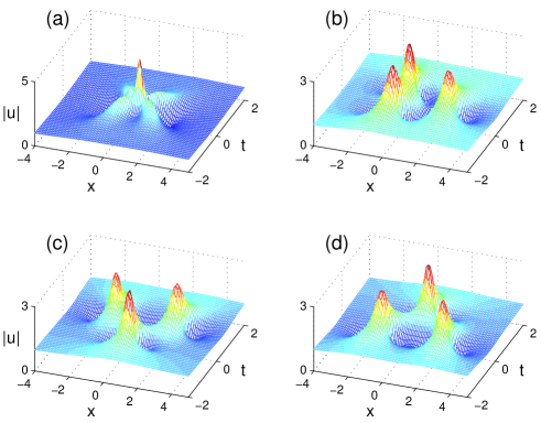
Figure 1: Second-order rogue waves with parameters: (a) $a_{3}=-1/12$; (b) $a_{3}=5/3$; (c) $a_{3}=-5i/2$; (d) $a_{3}=5i/2$.

Next we examine third-order rogue waves. In this case, we set $a_{1}=a_{2}=a_{4}=0$ without loss of generality. If one takes

$$a_{3}=-1/12,\quad a_{5}=-1/240,$$

then the corresponding solution $u_{m}(x,t)$ is equal to the third-order rogue wave obtained by Akhmediev et al. [9] except a shift in $x$. This solution is displayed in Fig. 2(a). The maximum amplitude of this solution is equal to 7, which occurs at $(x,t)=(1/2,0)$. We have found that this special rogue-wave solution $u_{m}(x,t)$ is also the one with the highest peak amplitude among all third-order rogue waves $u(x,t;a_{3},a_{5})$. But if we take other $(a_{3},a_{5})$ values, rogue waves with dynamics different from Fig. 2(a) will be obtained. Three of such solutions, with $(a_{3},a_{5})=(25/3,0)$, $(-25i/3,0)$ and $(0,50i/3)$, are displayed in Fig. 2(b,c,d) respectively. These solutions feature six intensity humps which appear at different times and/or space, and each intensity hump is roughly a first-order rogue wave (32). In Fig. 2(b), the solution exhibits triple temporal bumps at $x\approx-2$, double temporal bumps at $x\approx 2$, and a single temporal bump at $x\approx 6$. In Fig. 2(c), the solution develops a single hump first. Then this hump decays, but two new humps rise simultaneously at the two sides. Then these two humps decay, but three additional humps develop simultaneously. In Fig. 2(d), two intensity humps rise simultaneously at different spatial locations first. After they decay, additional four intensity humps arise at different locations and times. A remarkable feature in the rogue waves in Fig. 2(b-d) is the high regularity of their spatiotemporal patterns. For instance, the pattern in Fig. 2(c) is a highly symmetric triangle, while the one in Fig. 2(d) is like a pentagon. These spatiotemporal patterns of rogue waves are different from the ones reported in [11, 12].

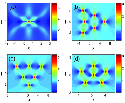
Figure 2: Third-order rogue waves with parameters $(a_{3},a_{5})$ as: (a) $(-1/12,-1/240)$; (b) $(25/3,0)$; (c) $(-25i/3,0)$; (d) $(0,50i/3)$.

The results shown above apparently can be extended to fourth- and higher-order rogue waves. By special choices of the free parameters $(a_{3},a_{5},a_{7},\cdots)$, we can reproduce the rogue waves obtained in [9] as special cases. But other choices of those parameters can yield even richer spatiotemporal patterns, such as triangular patterns like Fig. 2(c) but with more intensity humps such as 10, 15, and so on.

5 Summary and discussion

In this paper, we derived general $N$-th order rogue waves in the NLS equation by the bilinear method. These solutions were obtained from Gram determinant solutions of bilinear equations through dimension reduction and then further simplified to a very explicit form. We showed that these general rogue waves contain $N-1$ free irreducible complex parameters. By different choices of these free parameters, we obtained rogue waves with novel spatiotemporal patterns. These new spatiotemporal patterns reveal the rich dynamics in rogue-wave solutions and deepen our understanding of the rogue-wave phenomena. We also showed that the rogue waves reported in [9] are special solutions with the highest peak amplitude among all rogue waves of the same order.

We would like to point out that the new spatiotemporal patterns of rogue waves obtained in this paper may also find applications in other branches of applied mathematics and physics. For instance, the triangular rogue-wave patterns in Figs. 1(c), 2(c) and their higher-order extensions (with more intensity humps) closely resemble the spike pattern which forms after the point of gradient catastrophe in the semiclassical (zero-dispersion) limit of the NLS equation (see Fig. 1 in [20]). The connection between these exact rogue-wave solutions and the semiclassical-NLS patterns is an interesting question which lies outside the scope of the present article.

References

[1]O
[2] D. R. Solli, C. Ropers, P. Koonath and B. Jalali,
“Optical rogue waves”, Nature 450, 1054-1057 (2007).
[3]
B. Kibler, J. Fatome, C. Finot, G. Millot, F. Dias, G. Genty, N.
Akhmediev, J.M. Dudley, “The Peregrine soliton in nonlinear fibre
optics”, Nature Physics, 6, 790-795 (2010).
[4]
D.J. Benney and A.C. Newell, “Nonlinear wave envelopes”, J. Math.
Phys. 46, 133 (1967).
[5]
V.E. Zakharov, “Stability of periodic waves of finite amplitude on
the surface of a deep fluid,” J. Appl. Mech. Tech. Phys. 9, 190-94
(1968).
[6]
A. Hasegawa and F. Tappert, “Transmission of stationary nonlinear
optical pulses in dispersive dielectric fibers”, Appl. Phys. Lett.
23, 142 (1973).
[7]
V.E. Zakharov and A.B. Shabat, “Exact theory of two-dimensional
self-focusing and one-dimensional self-modulation of waves in
nonlinear media”, Sov. Phys. JETP 34, 62 (1972).
[8]
D. H. Peregrine, “Water waves, nonlinear Schrödinger equations
and their solutions,” J. Australian Math. Soc. B, 25, 16-43 (1983).
[9]
N. Akhmediev, A. Ankiewicz, and J. M. Soto-Crespo, “Rogue Waves and
Rational Solutions of the Nonlinear Schr dinger Equation,” Phys.
Rev. E 80, 026601 (2009).
[10]
P. Dubard, P. Gaillard, C. Klein, V.B. Matveev, “On multi-rogue
wave solutions of the NLS equation and positon solutions of the KdV
equation”, Eur. Phys. J. Special Topics 185, 247258 (2010).
[11]
P. Dubard, V.B. Matveev, “Multi-rogue waves solutions to the
focusing NLS equation and the KP-I equation”, Nat. Hazards. Earth.
Syst. Sci. 11, 667-672 (2011).
[12]
P. Gaillard, “Families of quasi-rational solutions of the NLS
equation and multi-rogue waves”, J. Phys. A: Math. Theor. 44, 435204
(2011).
[13]
M.J. Ablowitz and B.M Herbst, “On homoclinic structure and
numerically induced chaos for the nonlinear Schr6dinger equation”,
SIAM J. Appl. Math. 50, 339 (1990).
[14]
N. Akhmediev, A. Ankiewicz and M. Taki, “Waves that appear from
nowhere and disappear without a trace”, Phys. Lett. A 373, 675-678
(2009).
[15]
N. Akhmediev, J. M. Soto-Crespo and A. Ankiewicz, “Extreme waves
that appear from nowhere: on the nature of rogue waves”, Phys. Lett.
A, 373 2137-2145 (2009).
[16]
R. Hirota, The direct method in soliton theory (Cambridge
University Press, Cambridge, 2004).
[17]
M. Sato,
“Soliton equations as dynamical systems on a infinite dimensional
Grassmann manifolds”,
RIMS Kokyuroku, 439, 30 (1981).
[18]
M. Jimbo and T. Miwa,
“Solitons and infinite dimensional Lie algebras”,
Publ. RIMS, Kyoto Univ., 19, 943 (1983).
[19]
T. Ikeda and H.-F. Yamada,
“Polynomial -functions of the NLS-Toda hierarchy and
the Virasoro singular vectors”,
Lett. Math. Phys., 60, 147 (2002).
[20]
M. Bertola and A. Tovbis, “Universality for the focusing nonlinear
Schrödinger equation at the gradient catastrophe point: Rational
breathers and poles of the tritronquee solution to Painleve I”,
arXiv:1004.1828 (2010).