Ashkin-Teller criticality and pseudo first-order behavior
in a frustrated Ising model on the square lattice

Abstract

We study the challenging thermal phase transition to stripe order in the frustrated square-lattice Ising model with couplings $J_{1}<0$ (nearest-neighbor, ferromagnetic) and $J_{2}>0$ (second-neighbor, antiferromagnetic) for $g=J_{2}/|J_{1}|>1/2$. Using Monte Carlo simulations and known analytical results, we demonstrate Ashkin-Teller criticality for $g\geq g^{*}$, i.e., the critical exponents vary continuously between those of the $4$-state Potts model at $g=g^{*}$ and the Ising model for $g\to\infty$. Thus, stripe transitions offer a route to realizing a related class of conformal field theories with conformal charge $c=1$ and varying exponents. The transition is first-order for $g<g^{*}=0.67\pm 0.01$, much lower than previously believed, and exhibits pseudo first-order behavior for $g^{*}\leq g\lesssim 1$.

Breaking a four-fold symmetry (Z₄) at a thermal phase transition in a two-dimensional (2D) system can lead to a very special kind of critical behavior, where the critical exponents depend on microscopic details, in contrast to the universal exponents at normal transitions. Continuously varying exponents are possible in conformal field theory (CFT) when the conformal charge $c\geq 1$ Friedan ; Cardybook . A well-known microscopic Z₄-symmetric model realizes this behavior for $c=1$; the Ashkin-Teller (AT) model AToriginal ; AT consisting of two square-lattice Ising models coupled by a four-spin interaction. A Z₄-symmetric order parameter also obtains in the standard ferromagnetic Ising model when sufficiently strong frustrating (antiferromagnetic) second-neighbor couplings are added, in which case the low-temperature ordered state exhibits stripes of alternating magnetization (which can be arranged in four different ways on the square lattice). While $c=1$ AT criticality has been suspected at the stripe transition, it has not been possible to demonstrate this convincingly for a wide range of couplings (only at very strong second-neighbor coupling, where the system reduces to two weakly coupled Ising models honecker1 ; honecker2 ). It has even been difficult to determine whether the transition is continuous or first-order Nightingale ; Swendsen ; Oitmaa ; Binder ; Landau ; LandauBinder ; variational1 ; variational2 ; honecker1 ; honecker2 . A convincing demonstration of robust $c=1$ criticality with varying exponents would be important, since stripe ordering can be achieved in many different systems Edlund and represents a more realistic route to $c=1$ and varying exponents than the somewhat artificial AT model.

Using Monte Carlo (MC) simulations of the frustrated Ising and AT models, along with known analytical results for the AT model, we here demonstrate $c=1$ scaling at the stripe transition, with continuously varying exponents matching those of the AT model. We also uncover a remarkable pseudo first-order behavior associated with this type of continuous phase transition, which had not been previously noticed and which led to wrong conclusions regarding the nature of the stripe transition.

The 2D frustrated Ising model with couplings $J_{1}<0$ (ferromagnetic) and $J_{2}>0$ (antiferromagnetic) is defined by the Hamiltonian

$$H=J_{1}\sum_{\langle ij\rangle}\sigma_{i}\sigma_{j}+J_{2}\sum_{\langle\langle ij\rangle\rangle}\sigma_{i}\sigma_{j},$$ (1)

where first and second (diagonal) neighbors on the square lattice are denoted by $\langle ij\rangle$ and $\langle\langle ij\rangle\rangle$, respectively, and $\sigma_{i}=\pm 1$. A stripe state obtains at low temperature ($T$) when the coupling ratio $g=J_{2}/|J_{1}|>1/2$. Even though this model represents one of the most natural and simple extensions of the standard 2D Ising model, its stripe transition remains highly controversial. The most basic question under debate is whether the transition is continuous for all $g>1/2$, or there is a line of first-order transitions up to a point $g^{*}$. The next issue is to establish the universality class of the continuous transitions. Early numerical and analytic approaches supported the idea that the transition is always continuous, but with the critical exponents changing with $g$. Some variational studies variational1 ; variational2 and recent MC studies honecker1 ; honecker2 have, however, found a line of first-order transitions for $1/2<g\lesssim 1$. A very recent MC study honecker2 used a double-peak structure in energy histograms to conclude that the transition is first-order at least up to $g=0.9$. For large $g$ the transition should be AT-like, based on an effective continuum theory of two weakly coupled Ising models honecker2 . For smaller $g$, the AT behavior could either continue down to the point at which the transition turns first-order (with the critical end-point of the AT line corresponding to the 4-state Potts model), or some other behavior that is beyond the AT description may apply instead. The MC results of Ref. honecker2, could not distinguish between these scenarios.

We show here that the stripe transition is first order in a much smaller range of couplings than claimed in Ref. honecker2, ; for $1/2<g<g^{*}$ with $g^{*}\approx 0.67$. For $g>g^{*}$ it is continuous and in the AT class. The exponents change continuously with $g$ as in the AT model AT , with $g^{*}$ corresponding to the $4$-state Potts model Baxter ; Salas and $g\rightarrow\infty$ to standard Ising universality AT . First-order indicators (necessary but not sufficient), e.g., multiple peaks in energy and order-parameter distributions, lead to over-estimation of the region of discontinuous transitions. As we will show, this is because the $4$-state Potts model and neighboring transitions in the AT model exhibit pseudo first-order behavior, though these transitions are known to be continuous AT . The Potts point had not been identified in previous works, and the pseudo first-order behavior was interpreted as actual first-order transitions.

Stripe transition.—The striped phase is characterized by a two-component order parameter $(m_{x},m_{y})$ with

$$m_{x}=\frac{1}{N}\sum_{i=1}^{N}\sigma_{i}(-1)^{x_{i}},\mbox{~{}~{}~{}}m_{y}=\frac{1}{N}\sum_{i=1}^{N}\sigma_{i}(-1)^{y_{i}},$$ (2)

where $(x_{i},y_{i})$ are the coordinates of site $i$ on an $L\times L$ periodic lattice and $N=L^{2}$. We define $m^{2}=m_{x}^{2}+m_{y}^{2}$ and the stripe susceptibility $\chi=N(\langle m^{2}\rangle-\langle|m|\rangle^{2})/T$. We employ the standard single-spin Metropolis MC algorithm and use $|J_{1}|=1$ as the unit of $T$.

We analyze the peak value $C_{\rm max}(L)$ of the specific heat and $\chi_{\rm max}(L)$ of the stripe susceptibility. By standard finite-size scaling arguments Goldenfeld , $C_{\rm max}(L)\sim L^{\alpha/\nu}$ and $\chi_{\rm max}(L)\sim L^{\gamma/\nu}$. For first-order 2D transitions these quantities should instead diverge as $L^{2}$. Examples of the scaling behavior are shown in Fig 1. For the $L\leq 256$ systems studied, the exponent $\alpha/\nu$, estimated from the slope on the log-log scale, decreases with increasing $g$ (it is close to $2$ for $g=0.51$), while $\gamma/\nu$ remains close to $7/4$ for the $g$-values displayed here (also approaching $2$ closer to $g=1/2$). These behaviors can be affected by scaling corrections, and the slopes for moderate sizes may not reflect the true exponents. Fig. 1 also shows results for the $4$-state Potts model, for which it is rigorously known that $\alpha/\nu=1$ and $\gamma/\nu=7/4$, but there are multiplicative logarithmic scaling corrections that affect the behavior strongly for lattices accessible in MC simulations Salas . For $g$ in the range $0.66-0.70$, the $J_{1}$-$J_{2}$ scaling agrees well (up to factors) with that of the Potts model.

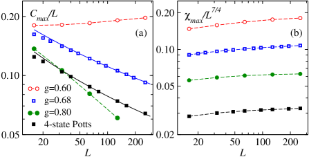
Figure 1: (Color online) Peak value of the specific heat and stripe susceptibility vs $L$ for the $J_{1}$-$J_{2}$ and $4$-state Potts models. Factors corresponding the asymptotic Potts scaling have been divided out. In (a) the curves through the $g=0.68$ and Potts data are fits to the Potts form $C=aL\ln(L/b)^{-3/2}$. A log-correction should also be present in (b) but the expected Potts form $\chi=aL^{7/4}\ln(L/b)^{-1/8}$ Salas is not seen for $L\leq 256$.

According to CFT Friedan ; Cardybook , the exponents can change continuously when the ordered phase breaks Z₄ symmetry. There are two known microscopic scenarios, exemplified by: (i) The XY model in a four-fold anisotropy field $h_{4}$. For $h_{4}=0$ there is a Kosterlitz-Thouless transition Berezinskii ; KT , while $|h_{4}|\rightarrow\infty$ gives standard Ising universality JKKN . (ii) The line of fixed points connecting the Ising and $4$-state Potts points in the square-lattice AT model AToriginal ; AT . Assuming that one of these scenarios applies to the continuous transitions in the $J_{1}$-$J_{2}$ model, $\gamma/\nu=7/4$ is fixed because this holds always for both (i) and (ii). This explains why $\chi/L^{7/4}$ is almost constant for all cases in Fig. 1(b). However, the observed variation of $\alpha/\nu$ with $g$ in Fig. 1(a) (and at larger $g$) rules out scenario (i), since $\alpha=0$ for all the fixed points there. Then the natural scenario left to consider is that there is a line of fixed points corresponding the AT model.

The AT Hamiltonian can be written as

$$H=-\sum_{\langle ij\rangle}(\sigma_{i}\sigma_{j}+\tau_{i}\tau_{j}+K\sigma_{i}\sigma_{j}\tau_{i}\tau_{j}),$$ (3)

where two Ising variables, $\sigma_{i},\tau_{i}$, reside on each site $i$ and are coupled to each other through $K$. The ferromagnetic phase of the AT model ($\langle\sigma\tau\rangle\neq 0$ and $\langle\sigma\rangle=\pm\langle\tau\rangle$) breaks Z₄ symmetry and the order parameter can again be expressed as a vector $(m_{\sigma},m_{\tau})$ with

$$m_{\sigma}=\frac{1}{N}\sum_{i=1}^{N}\sigma_{i},\mbox{~{}~{}~{}~{}}m_{\tau}=\frac{1}{N}\sum_{i=1}^{N}\tau_{i}.$$ (4)

The relevant Z₄ transitions take place when $K\in[0,1]$, where $K=0$ corresponds to two decoupled Ising models and $K=1$ can be mapped to the $4$-state Potts model. The $T>0$ transitions for $K\in[0,1]$ are all continuous, with the exponents depending on $K$ (but $\eta=1/4$ always) AT .

Binder cumulant.—To further understand the nature of the phase transitions, we probe the Binder cumulant of the stripe order parameter. For a $2$-component vector order-parameter, the cumulant is defined as

$$U=2\left(1-\frac{1}{2}\frac{\langle m^{4}\rangle}{\langle m^{2}\rangle^{2}}\right),$$ (5)

where the factors are chosen to make $U\rightarrow 0$ in the disordered phase and $U\rightarrow 1$ in the ordered phase in the thermodynamic limit. We define $U$ for the AT model in the same way, by using $m^{2}=m_{\sigma}^{2}+m_{\tau}^{2}$.

For continuous transitions, the cumulant typically grows monotonically upon lowering $T$ and stays bounded within $[0,1]$. It approaches a step function at $T_{c}$ as $L\to\infty$ Binder_c . For a first-order transition, it instead shows a non-monotonic behavior with $T$ for large systems Vollmayr , developing a negative peak which approaches $T_{c}$ and grows narrower and diverges as $L^{2}$ (in two dimensions) when $L\to\infty$. The nonmonotonic behavior can be traced to the emergence of multiple peaks in the order-parameter distribution (reflecting phase coexistence), as discussed in the context of the $J_{1}$-$J_{2}$ model in Sandvik10 .

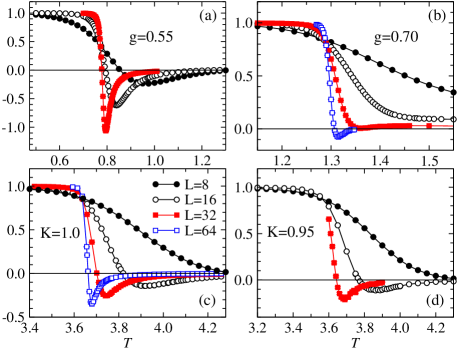
Figure 2: (Color online) Binder cumulant vs temperature for (a,b) the $J_{1}$-$J_{2}$ model at $g=0.55$ and $0.70$, and (c,d) the AT model at $K=1$ (the $4$-state Potts point) and $K=0.95$.

As is clear from Figs. 2(a,b), $U(T)$ of the $J_{1}$-$J_{2}$ model indeed develops a negative peak that grows with increasing $L$ for $g=0.55$ and $g=0.70$. As $g$ increases, the system sizes needed to observe a peak also increase, indicating a weakening discontinuity of $m$. The dependence of the peak value $U_{\rm min}$ on $L$ is shown in Fig. 3 for several values of $g$ (where $U_{\rm min}>0$ corresponds to a local minimum). Interpolating these data, we can extract a length $L_{0}(g)$ where $U_{\rm min}$ crosses zero for given $g$. $L_{0}(g)$ grows with increasing $g$ and diverges when $g\approx 0.82$ (i.e., for larger $g$ there is no negative peak). The vanishing of the negative peak might be taken as an estimate of the location $g^{*}$ of the multicritical point. One could also examine the $L(g)$ at which a minimum in $U(T)$ first forms (but is not yet negative). This gives a still higher value of $g^{*}$. However, such procedures, or ones based on multiple peaks in the order-parameter or energy distribution, over-estimate $g^{*}$ because these features can appear also for continuous transitions. Indeed, as shown in Figs 2(c,d) and 3, we observe negative cumulant peaks also in the Potts and AT models, in spite of these models being rigorously known to have continuous transitions.

The most natural scenario suggested by these data is again that the $J_{1}$-$J_{2}$ model at a point $g=g^{*}$ corresponds to the $4$-state Potts model. It therefore exhibits pseudo first-order behavior for some range of $g$-values above $g^{*}$, just like the AT model does for $K$ at and slightly below the Potts point $K=1$. The very similar behavior of $C_{\rm max}(L)$ for $g=0.68$ and the $4$-state Potts model in Fig. 1(a) already suggests $g^{*}\approx 0.68$. Below we will present further evidence of $g^{*}=0.67\pm 0.01$ indeed being a $4$-state Potts-universal point.

We presume that the stripe transition is first-order for $g<g^{*}$, instead of some alternative (and unlikely) exotic behavior outside known scenarios for Z₄ symmetry-breaking. The discontinuities are always very weak, however, so that the asymptotic first-order scaling behavior cannot be observed in practice. For instance, the negative $U(T)$ peak for $g<g^{*}$ and the specific heat appear to diverge much slower than the expected $L^{2}$ form. Similar behavior can also be observed for the $5$-state Potts model, which is a well-known prototypical example of a weak first-order transition Baxter with anomalously large correlation length $\xi$ Peczak . To observe clear first-order scaling, one has to use lattices with $L\gg\xi$.

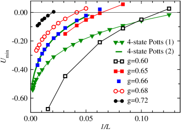
Figure 3: (Color online) Peak value of the Binder cumulant vs $L$ for the $J_{1}$-$J_{2}$ model at different $g$ values and the $4$-state Potts model. For the latter (1) in the legend refers to the original data and (2) has rescaled size, $L\to aL$, with $a\approx 2.36$.

Histograms—We next examine in some more detail the pseudo first-order signals in the AT and $J_{1}$-$J_{2}$ models, using the probability distribution of the order parameter and the energy. Some aspects of the full distribution $P(m_{x},m_{y})$ were discussed in Sandvik10 . Here we consider $P(m^{2})$. It is well known that phase coexistence at a first-order transition leads to a double-peak distribution in a narrow window (of size $\sim 1/L^{2}$ in two dimensions) around $T_{c}$. For $L\to\infty$, the distribution approaches two delta-functions (at $m=0$ and the value $\bar{m}$ of the order-parameter just below $T_{c}$), with weight shifting between the two across the narrow $T_{c}$ window. A double peak in the energy distribution corresponds to latent heat.

As would be expected based on the negative Binder cumulants, the pseudo first-order behavior also gives rise to double peaks in the order-parameter and energy distributions close to the transition. This is shown in Figs. 4(a,b) for the $4$-state Potts model. Similar behavior can be seen in the $J_{1}$-$J_{2}$ model, for which results are shown in Figs. 4(c,d) at $g=0.67\approx g^{*}$ (where the transition should be weakly first-order). In Ref. honecker2 a double-peaked energy histogram was seen all the way up to $g=0.9$ on large lattices. This was taken as a first-order transition, while our results show that this is merely pseudo first-order behavior Schreiber . Combining the results, we conclude that there is pseudo first-order behavior in the $J_{1}$-$J_{2}$ model from the Potts point $g^{*}\approx 0.67$ up to at least $g=0.9$.

Potts point.—If the continuous transitions indeed belong to the AT class for $g\in[g^{*},\infty]$, then a way to estimate the Potts point $g^{*}$ more precisely is to use the universal Binder crossing value $U^{*}$ (see Fig. 2) of curves $U(T)$ for different $L$ at fixed $g$. For the $4$-state Potts model (the $K=1$ AT model), we estimate $U^{*}=0.792(4)$ by extracting crossing points between data for pairs $(L,2L)$ and extrapolating to $L=\infty$. Examples of the finite-size scaling of crossing points are shown in Fig 5(a). In the $J_{1}$-$J_{2}$ model, $U^{*}(g)$ increases monotonically with $g$, as shown in Fig 5(b). We can now estimate $g^{*}$ by equating $U^{*}(g)$ to the $4$-state Potts value. This gives $g^{*}=0.67\pm 0.01$, in good agreement with the Potts-like behavior of the specific heat shown in Fig. 1(a) and the histograms in Fig. 4.

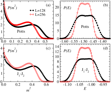
Figure 4: (Color online) Histograms of the order parameter $m^{2}$ and the energy $E$ for (a),(b) the 4-state Potts model (the $K=1$ AT model) and (c),(d) for the $J_{1}$-$J_{2}$ model at $g=0.67$. Here $T$ is very close to $T_{c}$, chosen such that the two peaks in the energy histograms are of the same height; for the Potts model $T/K=3.64231$ for $L=128$ and $3.64460$ for $L=256$, while for the $J_{1}$-$J_{2}$ model $T/J_{1}=1.2014$ for $L=128$ and $1.2004$ for $L=256$.

As a further test, we use a method inspired by the flowgram technique kuklov : Since the order-parameter distribution should be universal (up to scale factors) at $T_{c}$ for a continuous transition, and the negative peak in $U(T)$ represents one aspect of this distribution ($U^{*}$ being another one) the value $U_{\rm min}(L)$ should either approach a universal value (as $U^{*}$ does) or diverge in a universal manner when $L\rightarrow\infty$. Then, $U_{\rm min}(L)$ for the $4$-state Potts model and the $J_{1}$-$J_{2}$ model at $g^{*}$ should, if the models are controlled by the same fixed point, collapse onto the same curve for large systems, once a rescaling $L\rightarrow aL$ is introduced for one of the models. This is indeed the case if, and only if, $g$ is close to the $g^{*}$ point estimated above. Scaled Potts data match best the $g=0.66$ curve in Fig. 3. It is not clear whether $U_{\rm min}$ here diverges very slowly or converges to a finite value.

Conclusions.—By combining many mutually consistent signals, we have demonstrated a point $g=g^{*}=0.67\pm 0.01$ at which the $J_{1}$-$J_{2}$ model is controlled by the $4$-state Potts fixed point. The scenario of the critical curve for $g\in[g^{*},\infty)$ being in one-to-one correspondence with that of the AT model for $K\in[1,0)$ is the only possibility consistent with known CFT scenarios and MC results. The pseudo first-order behavior uncovered here, along with the very weak first-order transitions for $g\in(1/2,g^{*})$, is what made it so difficult to correctly characterize the nature of the transitions until now.

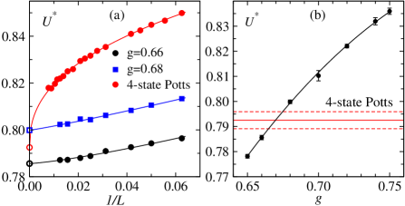
Figure 5: (Color online ) (a) Binder cumulant crossing points for $(L,2L)$ system pairs. The approach to $U^{*}(L=\infty)$ is expected to be governed by a nonuniversal scaling correction. The curves show fits of the form $U=a+b/L^{c}$. (b) $L\to\infty$ extrapolated $U^{*}$ of the $J_{1}$-$J_{2}$ model compared with the Potts result (the lines indicate the estimate with error bar).

With the nature of the transition now understood, it will be interesting to study other aspect of the model, i.e., the kinetics Shore ; Dominguez at the weakly first-order and pseudo first-order transitions. We also note that many interesting quantum problems involve the same kind of order-parameter symmetry in two dimensions, e.g., stripe states in models of high-$T_{c}$ superconductors White ; DelMaestro and valence-bond-solid states in quantum antiferromagnets Lou . The $T>0$ transitions in these systems, as well, may be impacted by the issues we have pointed out here. Acknowledgments.—We thank Bill Klein and Sid Redner for useful discussions. This work was supported in part by the NSF under Grant No. DMR-1104708.

References

- (1) D. Friedan, Z. Qiu, and S. Shenker, Phys. Rev. Lett. 52, 1575 (1984).
- (2) J. Cardy, Scaling and Renormalization in Statistical Physics (Cambridge University Press, 1996).
- (3) J. Ashkin and E. Teller, Phys. Rev. 64, 178 (1943); C. Fan and F. Y. Wu, Phys. Rev. B 2, 723 (1970); L. P. Kadanoff and F. J. Wegner, Phys. Rev. B 4, 3989 (1971).
- (4) S. Wiseman and E. Domany, Phys. Rev. E 48, 4080 (1993).
- (5) A. Kalz, A. Honecker, S. Fuchs, and T. Pruschke, Eur. Phys. J. B 65, 533 (2008).
- (6) A. Kalz, A. Honecker, and M. Moliner, Phys. Rev. B 84, 174407 (2011).
- (7) M. P. Nightingale, Phys. Lett. A 59, 486 (1977).
- (8) R. H. Swendsen and S. Krinsky, Phys. Rev. Lett. 43, 177 (1979).
- (9) J. Oitmaa, J. Phys. A: Math. Gen. 14, 1159 (1981).
- (10) K. Binder and D. P. Landau, Phys. Rev. B 21, 1941 (1980).
- (11) D. P. Landau, Phys. Rev. B 21, 1285 (1980).
- (12) D. P. Landau and K. Binder, Phys. Rev. B 31, 5946 (1985).
- (13) J. L. Moŕan-López, F. Aguilera-Granja, and J. M. Sanchez, Phys. Rev. B 48, 3519 (1993).
- (14) R. A. dos Anjos, J. R. Viana, and J. R. de Sousa, Phys. Lett. A 372, 1180 (2008).
- (15) E. Edlund and M. Nilsson Jacobi, Phys. Rev. Lett. 105, 137203 (2010).
- (16) R. J. Baxter, J. Phys. C: Solid State Phys. 6, L445 (1973).
- (17) J. Salas and A. D. Sokal, J. Stat. Phys. 88, 567 (1997).
- (18) N. Goldenfeld, Lectures on Phase transitions and the Renormalization Group (Addison-Wesley, Reading, MA, 1992).
- (19) V. L. Berezinskii, Sov. Phys.-JETP 32, 493 (1970).
- (20) J. M. Kosterlitz and D. J. Thouless, J. Phys. C: Solid State Phys. 6, 1181 (1973).
- (21) J. V. Jośe, L. P. Kadanoff, S. Kirkpatrick, and D. R. Nelson, Phys. Rev. B 16, 1217 (1977).
- (22) K. Binder, Phys. Rev. Lett. 47, 693 (1981).
- (23) K. Vollmayr, J. D. Reger, M. Scheucher, and K. Binder, Z. Phys. B 91, 113 (1993).
- (24) A. W. Sandvik, AIP Conf. Proc. 1297, 135 (2010) [arXiv:1101.3281].
- (25) P. Peczak and D.P.Landau, Phys. Rev. B 39, 11932 (1989).
- (26) Pseudo-first order behavior was previously observed in the energy distribution of the Baxter-Wu model, which is in the same universality class as the -state Potts model; N. Schreiber and J. Adler, J. Phys. A 38, 7253 (2005).
- (27) A. B. Kuklov, N. V. Prokof’ev, B. V. Svistunov, and M. Troyer, Ann. Phys. 321, 1602 (2006).
- (28) J. D. Shore, M. Holzer, and J. P. Sethna, Phys. Rev. 46, 11376 (1992).
- (29) R. Dominguez, K. M. Barros, and W. Klein, Phys. Rev. E, 79, 41121 (2009).
- (30) S. R. White and D. J. Scalapino. Phys. Rev. Lett. 91, 136403 (2003).
- (31) A. Del Maestro, B. Rosenow, and S. Sachdev, Phys. Rev. B 74, 024520 (2006).
- (32) J. Lou, A. W. Sandvik, and N. Kawashima, Phys. Rev. B 80, 180414 (2009); M. Tsukamoto, K. Harada, and N. Kawashima, J. Phys. Conf. Ser. 150, 042218 (2009).