A General Theory of Additive State Space Abstractions

Abstract

Informally, a set of abstractions of a state space $S$ is additive if the distance between any two states in $S$ is always greater than or equal to the sum of the corresponding distances in the abstract spaces. The first known additive abstractions, called disjoint pattern databases, were experimentally demonstrated to produce state of the art performance on certain state spaces. However, previous applications were restricted to state spaces with special properties, which precludes disjoint pattern databases from being defined for several commonly used testbeds, such as Rubik’s Cube, TopSpin and the Pancake puzzle. In this paper we give a general definition of additive abstractions that can be applied to any state space and prove that heuristics based on additive abstractions are consistent as well as admissible. We use this new definition to create additive abstractions for these testbeds and show experimentally that well chosen additive abstractions can reduce search time substantially for the (18,4)-TopSpin puzzle and by three orders of magnitude over state of the art methods for the 17-Pancake puzzle. We also derive a way of testing if the heuristic value returned by additive abstractions is provably too low and show that the use of this test can reduce search time for the 15-puzzle and TopSpin by roughly a factor of two.

1 Introduction

In its purest form, single-agent heuristic search is concerned with the problem of finding a least-cost path between two states (start and goal) in a state space given a heuristic function $h(t,g)$ that estimates the cost to reach the goal state $g$ from any state $t$. Standard algorithms for single-agent heuristic search such as $\textit{IDA}^{*}$ (?) are guaranteed to find optimal paths if $h(t,g)$ is admissible, i.e. never overestimates the actual cost to the goal state from $t$, and their efficiency is heavily influenced by the accuracy of $h(t,g)$. Considerable research has therefore investigated methods for defining accurate, admissible heuristics.

A common method for defining admissible heuristics, which has led to major advances in combinatorial problems (?, ?, ?, ?) and planning (?), is to “abstract” the original state space to create a new, smaller state space with the key property that for each path $\vec{p}$  in the original space there is a corresponding abstract path whose cost does not exceed the cost of $\vec{p}$. Given an abstraction, $h(t,g)$ can be defined as the cost of the least-cost abstract path from the abstract state corresponding to $t$ to the abstract state corresponding to $g$. The best heuristic functions defined by abstraction are typically based on several abstractions, and are equal to either the maximum, or the sum, of the costs returned by the abstractions (?, ?, ?).

The sum of the costs returned by a set of abstractions is not always admissible. If it is, the set of abstractions is said to be “additive”. The main contribution of this paper is to identify general conditions for abstractions to be additive. The new conditions subsume most previous notions of “additive” as special cases. The greater generality allows additive abstractions to be defined for state spaces that had no additive abstractions according to previous definitions, such as Rubik’s Cube, TopSpin, the Pancake puzzle, and related real-world problems such as the genome rearrangement problem described by ? (?). Our definitions are fully formal, enabling rigorous proofs of the admissibility and consistency of the heuristics defined by our abstractions. Heuristic $h(t,g)$ is consistent if for all states $t$, $g$ and $u,h(t,g)\leq cost(t,u)+h(u,g)$, where $cost(t,u)$ is the cost of the least-cost path from $t$ to $u$.

The usefulness of our general definitions is demonstrated experimentally by defining additive abstractions that substantially reduce the CPU time needed to solve TopSpin and the Pancake puzzle. For example, the use of additive abstractions allows the 17-Pancake puzzle to be solved three orders of magnitude faster than previous state-of-the-art methods.

Additional experiments show that additive abstractions are not always the best abstraction method. The main reason for this is that the solution cost calculated by an individual additive abstraction can sometimes be very low. In the extreme case, which actually arises in practice, all problems can have abstract solutions that cost 0. The final contribution of the paper is to introduce a technique that is sometimes able to identify that the sum of the costs of the additive abstractions is provably too small (“infeasible”).

The remainder of the paper is organized as follows. An informal introduction to abstraction is given in Section 2. Section 3 presents formal general definitions for abstractions that extend to general additive abstractions. We provide lemmas proving the admissibility and consistency of both standard and additive heuristics based on these abstractions. This section also discusses the relation to previous definitions. Section 4 describes successful applications of additive abstractions to TopSpin and the Pancake puzzle. Section 5 discusses the negative results. Section 6 introduces “infeasibility” and presents experimental results showing its effectiveness on the sliding tile puzzle and TopSpin. Conclusions are presented in Section 7.

2 Heuristics Defined by Abstraction

To illustrate the idea of abstraction and how it is used to define heuristics, consider the well-known 8-puzzle (the $3\times 3$ sliding tile puzzle). In this puzzle there are $9$ locations in the form of a $3\times 3$ grid and $8$ tiles, numbered 1–8, with the $9^{th}$ location being empty (or blank). A tile that is adjacent to the empty location can be moved into the empty location; every move has a cost of 1. The most common way of abstracting this state space is to treat several of the tiles as if they were indistinguishable instead of being distinct (?). An extreme version of this type of abstraction is shown in Figure 1. Here the tiles are all indistinguishable from each other, so an abstract state is entirely defined by the position of the blank. There are therefore only 9 abstract states, connected as shown in Figure 1. The goal state in the original puzzle has the blank in the upper left corner, so the abstract goal is the state shown at the top of the figure. The number beside each abstract state is the distance from the abstract state to the abstract goal. For example, in Figure 1, abstract state $e$ is 2 moves from the abstract goal. A heuristic function $h(t,g)$ for the distance from state $t$ to $g$ in the original space is computed in two steps: (1) compute the abstract state corresponding to $t$ (in this example, this is done by determining the location of the blank in state $t$); and then (2) determine the distance from that abstract state to the abstract goal. The calculation of the abstract distance can either be done in a preprocessing step to create a heuristic lookup table called a pattern database (?, ?) or at the time it is needed (?, ?, ?).

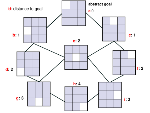
Figure 1: An abstraction of the 8-puzzle. The white square in each state is the blank and the non-white squares are the tiles, which are all indistinguishable from each other in this abstraction.

Given several abstractions of a state space, the heuristic $h_{max}(t,g)$ can be defined as the maximum of the abstract distances for $t$ given by the abstractions individually. This is the standard method for defining a heuristic function given multiple abstractions (?). For example, consider state $A$ of the $3\times 3$ sliding tile puzzle shown in the top left of Figure 2 and the goal state shown below it. The middle column shows an abstraction of these two states ($A_{1}$ and $g_{1}$) in which tiles 1, 3, 5, and 7, and the blank, are distinct while the other tiles are indistinguishable from each other. We refer to the distinct tiles as “distinguished tiles” and the indistinguishable tiles as “don’t care” tiles. The right column shows the complementary abstraction, in which tiles 1, 3, 5, and 7 are the “don’t cares” and tiles 2, 4, 6, and 8 are distinguished. The arrows in the figure trace out a least-cost path to reach the abstract goal $g_{i}$ from state $A_{i}$ in each abstraction. The cost of solving $A_{1}$ is 16 and the cost of solving $A_{2}$ is 12. Therefore, $h_{max}(A,g)$ is 16, the maximum of these two abstract distances.

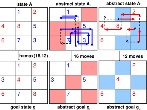
Figure 2: Computation of $h_{max}(A,g)$, the standard, maximum-based heuristic value for state $A$ (top left) using the two abstractions shown in the middle and right columns. Solid arrows denote distinguished moves, dashed arrows denote “don’t care” moves.

2.1 Additive Abstractions

Figure 3 illustrates how additive abstractions can be defined for the sliding tile puzzle (?, ?, ?). State $A$ and the abstractions are the same as in Figure 2, but the costs of the operators in the abstract spaces are defined differently. Instead of all abstract operators having a cost of 1, as was the case previously, an operator only has a cost of 1 if it moves a distinguished tile; such moves are called “distinguished moves” and are shown as solid arrows in Figures 2 and 3. An operator that moves a “don’t care” tile (a “don’t care” move) has a cost of 0 and is shown as a dashed arrow in the figures. Least-cost paths in abstract spaces defined this way therefore minimize the number of distinguished moves without considering how many “don’t care” moves are made. For example, the least-cost path for $A_{1}$ in Figure 3 contains fewer distinguished moves (9 compared to 10) than the least-cost path for $A_{1}$ in Figure 2—and is therefore lower cost according to the cost function just described—but contains more moves in total (18 compared to 16) because it has more “don’t care” moves (9 compared to 6). As Figure 3 shows, 9 distinguished moves are needed to solve $A_{1}$ and 5 distinguished moves are needed to solve $A_{2}$. Because no tile is distinguished in both abstractions, a move that has a cost of 1 in one space has a cost of 0 in the other space, and it is therefore admissible to add the two distances. The heuristic calculated using additive abstractions is referred to as $h_{add}$; in this example, $h_{add}(A,g)=9+5=14$. Note that $h_{add}(A,g)$ is less than $h_{max}(A,g)$ in this example, showing that heuristics based on additive abstractions are not always superior to the standard, maximum-based method of combining multiple abstractions even though in general they have proven very effective on the sliding tile puzzles (?, ?, ?).

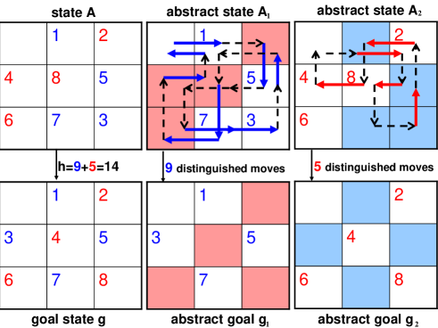
Figure 3: Computation of $h_{add}(A,g)$, the additive heuristic value for state $A$. Solid arrows denote distinguished moves, dashed arrows denote “don’t care” moves.

The general method defined by Korf, Felner, and colleagues (?, ?, ?) creates a set of $k$ additive abstractions by partitioning the tiles into $k$ disjoint groups and defining one abstraction for each group by making the tiles in that group distinguished in the abstraction. An important limitation of this and most other existing methods of defining additive abstractions is that they do not apply to spaces in which an operator can move more than one tile at a time, unless there is a way to guarantee that all the tiles that are moved by the operator are in the same group.

An example of a state space that has no additive abstractions according to previous definitions is the Pancake puzzle. In the $N$-Pancake puzzle, a state is a permutation of $N$ tiles ($0,1,...,N-1$) and has $N-1$ successors, with the $l^{th}$ successor formed by reversing the order of the first $l+1$ positions of the permutation ($1\leq l\leq N-1$). For example, in the 4-Pancake puzzle shown in Figure 4, the state at the top of the figure has three successors, which are formed by reversing the order of the first two tiles, the first three tiles, and all four tiles, respectively. Because the operators move more than one tile and any tile can appear in any location there is no non-trivial way to partition the tiles so that all the tiles moved by an operator are distinguished in just one abstraction. Other common state spaces that have no additive abstractions according to previous definitions—for similar reasons—are Rubik’s Cube and TopSpin.

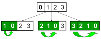
Figure 4: In the 4-Pancake puzzle each state has three successors.

The general definition of additive abstractions presented in the next section overcomes the limitations of previous definitions. Intuitively, abstractions will be additive provided that the cost of each operator is divided among the abstract spaces. Our definition provides a formal basis for this intuition. There are numerous ways to do this even when operators move many tiles (or, in other words, make changes to many state variables). For example, the operator cost might be divided proportionally across the abstractions based on the percentage of the tiles moved by the operator that are distinguished in each abstraction. We call this method of defining abstract costs “cost-splitting”. For example, consider two abstractions of the 4-Pancake puzzle, one in which tiles 0 and 1 are distinguished, the other in which tiles 2 and 3 are distinguished. Then the middle operator in Figure 4 would have a cost of $\frac{2}{3}$ in the first abstract space and $\frac{1}{3}$ in the second abstract space, because of the three tiles this operator moves, two are distinguished in the first abstraction and one is distinguished in the second abstraction.

A different method for dividing operator costs among abstractions focuses on a specific location (or locations) in the puzzle and assigns the full cost of the operator to the abstraction in which the tile that moves into this location is distinguished. We call this a “location-based” cost definition. In the Pancake puzzle it is natural to use the leftmost location as the special location since every operator changes the tile in this location. The middle operator in Figure 4 would have a cost of $0$ in the abstract space in which tiles 0 and 1 are distinguished and a cost of $1$ in the abstract space in which tiles 2 and 3 are distinguished because the operator moves tile 2 into the leftmost location.

Both these methods apply to Rubik’s Cube and TopSpin, and many other state spaces in addition to the Pancake puzzle, but the $h_{add}$ heuristics they produce are not always superior to the $h_{max}$ heuristics based on the same tile partitions. The theory and experiments in the remainder of the paper shed some light on the general question of when $h_{add}$ is preferable to $h_{max}$.

3 Formal Theory of Additive Abstractions

In this section, we give formal definitions and lemmas related to state spaces, abstractions, and the heuristics defined by them, and discuss their meanings and relation to previous work. The definitions of state space etc. in Section 3.1 are standard, and the definition of state space abstraction in Section 3.2 differs from previous definitions only in one important detail: each state transition in an abstract space has two costs associated with it instead of just one. The main new contribution is the definition of additive abstractions in Section 3.3.

The underlying structure of our abstraction definition is a directed graph (digraph) homomorphism. For easy reference, we quote here standard definitions of digraph and digraph homomorphism (?).

Definition 3.1

A digraph $G$ is a finite set $V=V(G)$ of vertices, together with a binary relation $E=E(G)$ on $V.$ The elements $(u,v)$ of E are called the arcs of G.

Definition 3.2

Let $G$ and $H$ be any digraphs. A homomorphism of $G$ to $H$, written as f : $G\rightarrow H$ is a mapping $f$: $V(G)\rightarrow V(H)$ such that $(f(u),f(v))\in E(H)$ whenever $(u,v)\in E(G)$.

Note that the digraphs $G$ and $H$ may have self-loops, $(u,u)$, and a homomorphism is not required to be surjective in either vertices or arcs. We typically refer to arcs as edges, but it should be kept in mind that, in general, they are directed edges, or ordered pairs.

3.1 State Space

Definition 3.3

A state space is a weighted directed graph ${\mathcal{S}}=\langle T,\Pi,C\rangle$ where $T$ is a finite set of states, $\Pi\subseteq T\times T$ is a set of directed edges (ordered pairs of states) representing state transitions, and $C:\Pi\longrightarrow{{\mathcal{N}}}=\{0,1,2,3,\dots\}$ is the edge cost function.

In typical practice, ${\mathcal{S}}$ is defined implicitly. Usually each distinct state in $T$ corresponds to an assignment of values to a set of state variables. $\Pi$ and $C$ derive from a successor function, or a set of planing operators. In some cases, $T$ is restricted to the set of states reachable from a given state. For example, in the 8-puzzle, the set of edges $\Pi$ is defined by the rule “a tile that is adjacent to the empty location can be moved into the empty location”, and the set of states $T$ is defined in one of two ways: either as the set of states reachable from the goal state, or as the set of permutations of the tiles and the blank, in which case $T$ consists of two components that are not connected to one another. The standard cost function $C$ for the 8-puzzle assigns a cost of $1$ to all edges, but it is easy to imagine cost functions for the 8-puzzle that depend on the tile being moved or the locations involved in the move.

A path from state $t$ to state $g$ is a sequence of edges beginning at $t$ and ending at $g$. Formally, $\vec{p}$ is a path from state $t$ to state $g$ if $\vec{p}=\langle\pi^{1},\dots,\pi^{n}\rangle,\pi^{j}\in\Pi$ where $\pi^{j}=(t^{j-1},t^{j}),j\in\{1,\dots,n\}$ and $t^{0}=t,t^{n}=g$. Note the use of superscripts rather than subscripts to distinguish states and edges within a state space. The length of $\vec{p}$ is the number of edges $n$ and its cost is $C(\vec{p})=\sum_{j=1}^{n}C(\pi^{j})$. We use $Paths({\mathcal{S}},t,g)$ to denote the set of all paths from $t$ to $g$ in ${\mathcal{S}}$.

Definition 3.4

The optimal (minimum) cost of a path from state $t$ to state $g$ in ${\mathcal{S}}$ is defined by

$${\mbox{\rm OPT}}(t,g)=\min_{\vec{p}\in Paths({\mathcal{S}},t,g)}C(\vec{p})$$

A pathfinding problem is a triple $\langle{\mathcal{S}},t,g\rangle$, where ${\mathcal{S}}$ is a state space and $t,g\in T$, with the objective of finding the minimum cost of a path from $t$ to $g$, or in some cases finding a minimum cost path $\vec{p}\in Paths({\mathcal{S}},t,g)$ such that $C(\vec{p})={\mbox{\rm OPT}}(t,g)$. Having just one goal state may seem restrictive, but problems having a set of goal states can be accommodated with this definition by adding a virtual goal state to the state space with zero-cost edges from the actual goal states to the virtual goal state.

3.2 State Space Abstraction

Definition 3.5

An Abstraction System is a pair $\langle{\mathcal{S}},\aleph\rangle$ where ${\mathcal{S}}=\langle T,\Pi,C\rangle$ is a state space and $\aleph=\{\langle{\mathcal{A}}_{i},\psi_{i}\rangle\;|\;\psi_{i}:{\mathcal{S}}\rightarrow{\mathcal{A}}_{i},1\leq i\leq k\}$ is a set of abstractions, where each abstraction is a pair consisting of an abstract state space and an abstraction mapping, where “abstract state space” and “abstraction mapping” are defined below.

Note that these abstractions are not intended to form a hierarchy and should be considered a set of independent abstractions.

Definition 3.6

An abstract state space is a directed graph with two weights per edge, defined by a four-tuple ${\mathcal{A}}_{i}=\langle T_{i},\Pi_{i},C_{i},R_{i}\rangle$.

$T_{i}$ is the set of abstract states and $\Pi_{i}$ is the set of abstract edges, as in the definition of a state space. In an abstract space there are two costs associated with each $\pi_{i}\in\Pi_{i}$, the primary cost $C_{i}:\Pi_{i}\longrightarrow{\mathcal{N}}$ and the residual cost $R_{i}:\Pi_{i}\longrightarrow{\mathcal{N}}$. The idea of having two costs per abstract edge, instead of just one, is inspired by the practice, illustrated in Figure 3, of having two types of edges in the abstract space and counting distinguished moves differently than “don’t care” moves. In that example, our primary cost is the cost associated with the distinguished moves, and our residual cost is the cost associated with the “don’t care” moves. The usefulness of considering the cost of “don’t care” moves arises when the abstraction system is additive, as suggested by Lemmas 3.6 and 3.10 below. These indicate when the additive heuristic is infeasible and can be improved, the effectiveness of which will become apparent in the experiments reported in Section 6.

Like edges, each abstract path $\vec{p}_{i}=\langle\pi^{1}_{i},\dots,\pi^{n}_{i}\rangle$ in ${\mathcal{A}}_{i}$ has a primary and residual cost: $C_{i}(\vec{p}_{i})=\sum_{j=1}^{n}C_{i}(\pi^{j}_{i})$, and $R_{i}(\vec{p}_{i})=\sum_{j=1}^{n}R_{i}(\pi^{j}_{i})$.

Definition 3.7

An abstraction mapping $\psi_{i}:{\mathcal{S}}\longrightarrow{\mathcal{A}}_{i}$ between state space ${\mathcal{S}}$ and abstract state space ${\mathcal{A}}_{i}$ is defined by a mapping between the states of ${\mathcal{S}}$ and the states of ${\mathcal{A}}_{i}$, $\psi_{i}:T\rightarrow T_{i}$, that satisfies the two following conditions.

The first condition is that the mapping is a homomorphism and thus connectivity in the original space is preserved, i.e.,

(1) $$\forall(u,v)\in\Pi,(\psi_{i}(u),\psi_{i}(v))\in\Pi_{i}$$

In other words, for each edge in the original space ${\mathcal{S}}$ there is a corresponding edge in the abstract space ${\mathcal{A}}_{i}$. Note that if $u\neq v$ and $\psi_{i}(u)=\psi_{i}(v)$ then a non-identity edge in ${\mathcal{S}}$ gets mapped to an identity edge (self-loop) in ${\mathcal{A}}_{i}$. We use the shorthand notation $t^{j}_{i}=\psi_{i}(t^{j})$ for the abstract state in $T_{i}$ corresponding to $t^{j}\in T$, and $\pi^{j}_{i}=\psi_{i}(\pi^{j})=(\psi_{i}(u^{j}),\psi_{i}(v^{j}))$ for the abstract edge in $\Pi_{i}$ corresponding to $\pi^{j}=(u^{j},v^{j})\in\Pi$.

The second condition that the state mapping must satisfy is that abstract edges must not cost more than any of the edges they correspond to in the original state space, i.e.,

(2) $$\forall\pi\in\Pi,C_{i}(\pi_{i})+R_{i}(\pi_{i})\leq C(\pi)$$

As a consequence, if multiple edges in the original space map to the same abstract edge $\rho\in\Pi_{i}$, as is usually the case, $C_{i}(\rho)+R_{i}(\rho)$ must be less than or equal to all of them, i.e.,

$$\forall\rho\in\Pi_{i},\ C_{i}(\rho)+R_{i}(\rho)\leq\min_{\pi\in\Pi,\psi_{i}(\pi)=\rho}C(\pi)$$

Note that if no edge maps to an edge in the abstract space, then no bound on the cost of that edge is imposed.

For example, the state mapping used to define the abstraction in the middle column of Figure 3 maps an 8-puzzle state to an abstract state by renaming tiles 2, 4, 6, and 8 to “don’t care”. This mapping satisfies condition (1) because “don’t care” tiles can be exchanged with the blank whenever regular tiles can. It satisfies condition (2) because each move is either a distinguished move ($C_{i}(\pi_{i})=1$ and $R_{i}(\pi_{i})=0$) or a “don’t care” move ($C_{i}(\pi_{i})=0$ and $R_{i}(\pi_{i})=1$) and in both cases $C_{i}(\pi_{i})+R_{i}(\pi_{i})=1$, the cost of the edge $\pi$ in the original space.

The set of abstract states $T_{i}$ is usually equal to $\psi_{i}(T)=\{\psi_{i}(t)\;|\;t\in T\}$, but it can be a superset, in which case the abstraction is said to be non-surjective (?). Likewise, the set of abstract edges $\Pi_{i}$ is usually equal to $\psi_{i}(\Pi)=\{\psi_{i}(\pi)\;|\;\pi\in\Pi\}$ but it can be a superset even if $T_{i}=\psi_{i}(T)$. In some cases, one deliberately chooses an abstract space that has states or edges that have no counterpart in the original space. For example, the methods that define abstractions by dropping operator preconditions must, by their very design, create abstract spaces that have edges that do not correspond to any edge in the original space (e.g. ?). In other cases, non-surjectivity is an inadvertent consequence of the abstract space being defined implicitly as the set of states reachable from the abstract goal state by applying operator inverses. For example, if a tile in the $2\times 2$ sliding tile puzzle is mapped to the blank in the abstract space, the puzzle now has two blanks and states are reachable in the abstract space that have no counterpart in the original space (?). For additional examples and an extensive discussion of non-surjectivity see the previous paper by ? (?).

All the lemmas and definitions that follow assume an abstraction system $\langle{\mathcal{S}},\aleph\rangle$ containing $k$ abstractions has been given. Conditions (1) and (2) guarantee the following.

Lemma 3.1

For any path $\vec{p}\in Paths({\mathcal{S}},u^{1},u^{2})$ in ${\mathcal{S}}$, there is a corresponding abstract path $\psi_{i}(\vec{p})$ from $u^{1}_{i}$ to $u^{2}_{i}$ in ${\mathcal{A}}_{i}$ and $C_{i}(\psi_{i}(\vec{p}))+R_{i}(\psi_{i}(\vec{p}))\leq C(\vec{p})$.

Proof: By definition, $\vec{p}\in Paths({\mathcal{S}},u^{1},u^{2})$ in ${\mathcal{S}}$ is a sequence of edges $\langle\pi^{1},\dots,\pi^{n}\rangle,\pi^{j}\in\Pi$ where $\pi^{j}=(t^{j-1},t^{j}),j\in\{1,\dots,n\}$ and $t^{0}=u^{1},t^{n}=u^{2}$. Because $\Pi_{i}\supseteq\psi_{i}(\Pi)$, each of the corresponding abstract edges exists ($\pi^{j}_{i}\in\Pi_{i}$). Because $\pi^{1}_{i}=(u^{1}_{i},t^{1}_{i})$ and $\pi^{n}_{i}=(t^{n-1}_{i},u^{2}_{i})$, the sequence $\psi_{i}(\vec{p})=\langle\pi^{1}_{i},\dots,\pi^{n}_{i}\rangle$ is a path from $u^{1}_{i}$ to $u^{2}_{i}$.

By definition, $C(\vec{p})=\sum_{j=1}^{n}C(\pi^{j})$. For each $\pi^{j}$, Condition (2) ensures that $C(\pi^{j})\geq C_{i}(\pi^{j}_{i})+R_{i}(\pi^{j}_{i})$, and therefore $C(\vec{p})\geq\sum_{j=1}^{n}(C_{i}(\pi^{j}_{i})+R_{i}(\pi^{j}_{i}))=\sum_{j=1}^{n}C_{i}(\pi^{j}_{i})+\sum_{j=1}^{n}R_{i}(\pi^{j}_{i})=C_{i}(\psi_{i}(\vec{p}))+R_{i}(\psi_{i}(\vec{p}))$.

For example, consider state $A$ and goal $g$ in Figure 3. Because of condition (1), any path from state $A$ to $g$ in the original space is also a path from abstract state $A_{1}$ to abstract goal state $g_{1}$ and from abstract state $A_{2}$ to $g_{2}$ in the abstract spaces. Because of condition (2), the cost of the path in the original space is greater than or equal to the sum of the primary cost and the residual cost of the corresponding abstract path in each abstract space.

We use $Paths({\mathcal{A}}_{i},u,v)$ to mean the set of all paths from $u$ to $v$ in space ${\mathcal{A}}_{i}$.

Definition 3.8

The optimal abstract cost from abstract state $u$ to abstract state $v$ in ${\mathcal{A}}_{i}$ is defined as

$${\mbox{\rm OPT}}_{i}(u,v)=\min_{\vec{q}\in Paths({\mathcal{A}}_{i},u,v)}C_{i}(\vec{q})+R_{i}(\vec{q})$$

Definition 3.9

We define the heuristic obtained from abstract space ${\mathcal{A}}_{i}$ for the cost from state $t$ to $g$ as

$$h_{i}(t,g)={\mbox{\rm OPT}}_{i}(t_{i},g_{i}).$$

Note that in these definitions, the path minimizing the cost is not required to be the image, $\psi_{i}(\vec{p})$, of a path $\vec{p}$ in ${\mathcal{S}}$.

The following prove that the heuristic generated by each individual abstraction is admissible (Lemma 3.2) and consistent (Lemma 3.3).

Lemma 3.2

$h_{i}(t,g)\leq{\mbox{\rm OPT}}(t,g)$ for all $t,g\in T$ and all $i\in\{1,\dots,k\}$.

Proof: By Lemma 3.1, $C(\vec{p})\geq C_{i}(\psi_{i}(\vec{p}))+R_{i}(\psi_{i}(\vec{p}))$, and therefore

$$\min_{\vec{p}\in Paths({\mathcal{S}},t,g)}C(\vec{p})\geq\min_{\vec{p}\in Paths({\mathcal{S}},t,g)}C_{i}(\psi_{i}(\vec{p}))+R_{i}(\psi_{i}(\vec{p})).$$

The left hand side of this inequality is ${\mbox{\rm OPT}}(t,g)$ by definition, and the right hand side is proved in the following Claim 3.2.1 to be greater than or equal to $h_{i}(t,g)$. Therefore, ${\mbox{\rm OPT}}(t,g)\geq h_{i}(t,g)$.

Claim 3.2.1 $\min_{\vec{p}\in Paths({\mathcal{S}},t,g)}C_{i}(\psi_{i}(\vec{p}))+R_{i}(\psi_{i}(\vec{p}))\geq h_{i}(t,g)$ for all $t,g\in T$.

Proof of Claim 3.2.1: By Lemma 3.1 for every path $\vec{p}$ there is a corresponding abstract path. There may also be additional paths in the abstract space, that is, $\{\psi_{i}(\vec{p})\;|\;\vec{p}\in Paths({\mathcal{S}},t,g)\}\subseteq Paths({\mathcal{A}}_{i},t_{i},g_{i})$. It follows that $\{C_{i}(\psi_{i}(\vec{p}))+R_{i}(\psi_{i}(\vec{p}))\;|\;\vec{p}\in Paths({\mathcal{S}},t,g)\}\subseteq\{C_{i}(\vec{q})+R_{i}(\vec{q})\;|\;\vec{q}\in Paths({\mathcal{A}}_{i},t_{i},g_{i})\}$. Therefore,

$$\min_{\vec{p}\in Paths({\mathcal{S}},t,g)}C_{i}(\psi_{i}(\vec{p}))+R_{i}(\psi_{i}(\vec{p}))\geq\min_{\vec{q}\in Paths({\mathcal{A}}_{i},t_{i},g_{i})}C_{i}(\vec{q})+R_{i}(\vec{q})={\mbox{\rm OPT}}_{i}(t_{i},g_{i})=h_{i}(t,g)$$

Lemma 3.3

$h_{i}(t^{1},g)\leq{\mbox{\rm OPT}}(t^{1},t^{2})+h_{i}(t^{2},g)$ for all $t^{1},t^{2},g\in T$ and all $i\in\{1,\dots,k\}$.

Proof: By the definition of ${\mbox{\rm OPT}}_{i}$ as a minimization and the definition of $h_{i}(t,g)$, it follows that $h_{i}(t^{1},g)={\mbox{\rm OPT}}_{i}(t^{1}_{i},g_{i})\leq{\mbox{\rm OPT}}_{i}(t^{1}_{i},t^{2}_{i})+{\mbox{\rm OPT}}_{i}(t^{2}_{i},g_{i})={\mbox{\rm OPT}}_{i}(t^{1}_{i},t^{2}_{i})+h_{i}(t^{2},g)$.

To complete the proof, we observe that by Lemma 3.2, ${\mbox{\rm OPT}}(t^{1},t^{2})\geq h_{i}(t^{1},t^{2})={\mbox{\rm OPT}}_{i}(t^{1}_{i},t^{2}_{i})$.

Definition 3.10

The $h_{max}$ heuristic from state $t$ to state $g$ defined by an abstraction system $\langle{\mathcal{S}},\aleph\rangle$ is

$$h_{max}(t,g)=\max_{i=1}^{k}h_{i}(t,g)$$

From Lemmas 3.2 and 3.3 it immediately follows that $h_{max}$ is admissible and consistent.

3.3 Additive Abstractions

In this section, we formalize the notion of “additive abstraction” that was introduced intuitively in Section 2.1. The example there showed that $h_{add}(t,g)$, the sum of the heuristics for state $t$ defined by multiple abstractions, was admissible provided the cost functions in the abstract spaces only counted the “distinguished moves”. In our formal framework, the “cost of distinguished moves” is captured by the notion of primary cost.

Definition 3.11

For any pair of states $t,g\in T$ the additive heuristic given an abstraction system is defined to be

$$h_{add}(t,g)=\sum_{i=1}^{k}C^{*}_{i}(t_{i},g_{i}).$$

where

$$C^{*}_{i}(t_{i},g_{i})=\min_{\vec{q}\in Paths({\mathcal{A}}_{i},t_{i},g_{i})}C_{i}(\vec{q})$$

is the minimum primary cost of a path in the abstract space from $t_{i}$ to $g_{i}$.

In Figure 3, for example, $C^{*}_{1}(A_{1},g_{1})=9$ and $C^{*}_{2}(A_{2},g_{2})=5$ because the minimum number of distinguished moves to reach $g_{1}$ from $A_{1}$ is $9$ and the minimum number of distinguished moves to reach $g_{2}$ from $A_{2}$ is $5$.

Intuitively, $h_{add}$ will be admissible if the cost of edge $\pi$ in the original space is divided among the abstract edges $\pi_{i}$ that correspond to $\pi$, as is done by the “cost-splitting” and “location-based” methods for defining abstract costs that were introduced at the end of Section 2.1. This leads to the following formal definition.

Definition 3.12

An abstraction system $\langle{\mathcal{S}},\aleph\rangle$ is additive if $\forall\pi\in\Pi,\sum_{i=1}^{k}C_{i}(\pi_{i})\leq C(\pi)$.

The following prove that $h_{add}$ is admissible (Lemma 3.4) and consistent (Lemma 3.5) when the abstraction system $\langle{\mathcal{S}},\aleph\rangle$ is additive.

Lemma 3.4

If $\langle{\mathcal{S}},\aleph\rangle$ is additive then $h_{add}(t,g)\leq{\mbox{\rm OPT}}(t,g)$ for all $t,g\in T$.

Proof: Assume that ${\mbox{\rm OPT}}(t,g)=C(\vec{p})$, where $\vec{p}=\langle\pi^{1},\dots,\pi^{n}\rangle\in Paths({\mathcal{S}},t,g)$. Therefore, ${\mbox{\rm OPT}}(t,g)=\sum_{j=1}^{n}C(\pi^{j})$. Since $\langle{\mathcal{S}},\aleph\rangle$ is additive, it follows by definition that

$$\sum_{j=1}^{n}C(\pi^{j}) \geq \sum_{j=1}^{n}\sum_{i=1}^{k}C_{i}(\pi_{i}^{j})=\sum_{i=1}^{k}\sum_{j=1}^{n}C_{i}(\pi_{i}^{j})$$

$$\geq \sum_{i=1}^{k}C^{*}_{i}(t_{i},g_{i})=h_{add}(t,g)$$

where the last line follows from the definitions of $C^{*}_{i}$ and $h_{add}$.

Lemma 3.5

If $\langle{\mathcal{S}},\aleph\rangle$ is additive then $h_{add}(t^{1},g)\leq{\mbox{\rm OPT}}(t^{1},t^{2})+h_{add}(t^{2},g)$ for all $t^{1},t^{2},g\in T$.

Proof: $C^{*}_{i}(t^{1}_{i},g_{i})$ obeys the triangle inequality: $C^{*}_{i}(t^{1}_{i},g_{i})\leq C^{*}_{i}(t^{1}_{i},t^{2}_{i})+C^{*}_{i}(t^{2}_{i},g_{i})$ for all $t^{1},t^{2},g\in T$. It follows that $\sum_{i=1}^{k}C^{*}_{i}(t^{1}_{i},g_{i})\leq\sum_{i=1}^{k}C^{*}_{i}(t^{1}_{i},t^{2}_{i})+\sum_{i=1}^{k}C^{*}_{i}(t^{2}_{i},g_{i})$.

Because $\sum_{i=1}^{k}C^{*}_{i}(t^{1}_{i},g_{i})=h_{add}(t^{1},g)$ and $\sum_{i=1}^{k}C^{*}_{i}(t^{2}_{i},g_{i})=h_{add}(t^{2},g)$, it follows that $h_{add}(t^{1},g)\leq\sum_{i=1}^{k}C^{*}_{i}(t^{1}_{i},t^{2}_{i})+h_{add}(t^{2},g)$.

Since $\langle{\mathcal{S}},\aleph\rangle$ is additive, by Lemma 3.4, ${\mbox{\rm OPT}}(t^{1},t^{2})\geq\sum_{i=1}^{k}C^{*}_{i}(t^{1}_{i},t^{2}_{i})$.

Hence $h_{add}(t^{1},g)\leq{\mbox{\rm OPT}}(t^{1},t^{2})+h_{add}(t^{2},g)$ for all $t^{1},t^{2},g\in T$.

We now develop a simple test that has important consequences for additive heuristics. Define $\vec{P}_{i}({t_{i}},{g_{i}})=\{\vec{q}\;|\;\vec{q}\in Paths({\mathcal{A}}_{i},t_{i},g_{i})$ and $C_{i}(\vec{q})=C^{*}_{i}(t_{i},g_{i})\}$, the set of abstract paths from $t_{i}$ to $g_{i}$ whose primary cost is minimal.

Definition 3.13

The conditional optimal residual cost is the minimum residual cost among the paths in $\vec{P}_{i}({t_{i}},{g_{i}})$:

$$R^{*}_{i}(t_{i},g_{i})=\min_{\vec{q}\in\vec{P}_{i}({t_{i}},{g_{i}})}R_{i}(\vec{q})$$

Note that the value of ($C^{*}_{i}(t_{i},g_{i})+R^{*}_{i}(t_{i},g_{i})$) is sometimes, but not always, equal to the optimal abstract cost ${\mbox{\rm OPT}}_{i}(t_{i},g_{i})$. In Figure 3, for example, ${\mbox{\rm OPT}}_{1}(A_{1},g_{1})=16$ (a path with this cost is shown in Figure 2) and $C^{*}_{1}(A_{1},g_{1})+R^{*}_{1}(A_{1},g_{1})=18$, while $C^{*}_{2}(A_{2},g_{2})+R^{*}_{2}(A_{2},g_{2})={\mbox{\rm OPT}}_{2}(A_{2},g_{2})=12$. As the following lemmas show, it is possible to draw important conclusions about $h_{add}$ by comparing its value to ($C^{*}_{i}(t_{i},g_{i})+R^{*}_{i}(t_{i},g_{i})$).

Lemma 3.6

Let $\langle{\mathcal{S}},\aleph\rangle$ be any additive abstraction system and let $t,g\in T$ be any states. If $h_{add}(t,g)\geq C^{*}_{j}(t_{j},g_{j})+R^{*}_{j}(t_{j},g_{j})$ for all $j\in\{1,\dots,k\}$, then $h_{add}(t,g)\geq h_{max}(t,g)$.

Proof: By the definition of ${\mbox{\rm OPT}}_{i}(t_{i},g_{i})$, $\forall j\in\{1,\dots,k\},C^{*}_{j}(t_{j},g_{j})+R^{*}_{j}(t_{j},g_{j})\geq{\mbox{\rm OPT}}_{j}(t_{j},g_{j})$. Therefore, $\forall j\in\{1,\dots,k\},h_{add}(t,g)\geq C^{*}_{j}(t_{j},g_{j})+R^{*}_{j}(t_{j},g_{j})\geq{\mbox{\rm OPT}}_{j}(t_{j},g_{j})\Rightarrow h_{add}(t,g)\geq\max_{1\leq i\leq k}{\mbox{\rm OPT}}_{i}(t_{i},g_{i})=h_{max}(t,g)$.

Lemma 3.7

For an additive $\langle{\mathcal{S}},\aleph\rangle$ and path $\vec{p}\in Paths({\mathcal{S}},t,g)$ with $C(\vec{p})=\sum_{i=1}^{k}C^{*}_{i}(t_{i},g_{i})$, $C_{j}(\psi_{j}(\vec{p}))=C^{*}_{j}(t_{j},g_{j})$ for all $j\in\{1,\dots,k\}$.

Proof: Suppose for a contradiction that there exists some $i_{1}$, such that $C_{i_{1}}(\psi_{i_{1}}(\vec{p}))>C^{*}_{i_{1}}(t_{i_{1}},g_{i_{1}})$. Then because $C(\vec{p})=\sum_{i=1}^{k}C^{*}_{i}(t_{i},g_{i})$, there must exist some $i_{2}$, such that $C_{i_{2}}(\psi_{i_{2}}(\vec{p}))<C^{*}_{i_{2}}(t_{i_{2}},g_{i_{2}})$, which contradicts the definition of $C^{*}_{i}$. Therefore, such an $i_{1}$ does not exist and $C_{j}(\psi_{j}(\vec{p}))=C^{*}_{j}(t_{j},g_{j})$ for all $j\in\{1,\dots,k\}$.

Lemma 3.8

For an additive $\langle{\mathcal{S}},\aleph\rangle$ and a path $\vec{p}\in Paths({\mathcal{S}},t,g)$ with $C(\vec{p})=\sum_{i=1}^{k}C^{*}_{i}(t_{i},g_{i})$, $R_{i}(\psi_{i}(\vec{p}))\geq R^{*}_{i}(t_{i},g_{i})$ for all $i\in\{1,\dots,k\}$.

Proof: Following Lemma 3.7 and the definition of $\vec{P}_{i}({t_{i}},{g_{i}})$, $\psi_{i}(\vec{p})\in\vec{P}_{i}({t_{i}},{g_{i}})$ for all $i\in\{1,\dots,k\}$. Because $R^{*}_{i}(t_{i},g_{i})$ is the smallest residual cost of paths in $\vec{P}_{i}({t_{i}},{g_{i}})$, it follows that $R_{i}(\psi_{i}(\vec{p}))\geq R^{*}_{i}(t_{i},g_{i})$.

Lemma 3.9

For an additive $\langle{\mathcal{S}},\aleph\rangle$ and a path $\vec{p}\in Paths({\mathcal{S}},t,g)$ with $C(\vec{p})=\sum_{i=1}^{k}C^{*}_{i}(t_{i},g_{i})$, $\sum_{i=1}^{k}C^{*}_{i}(t_{i},g_{i})\geq C^{*}_{j}(t_{j},g_{j})+R^{*}_{j}(t_{j},g_{j})$ for all $j\in\{1,\dots,k\}$.

Proof: By Lemma 3.1, $C(\vec{p})\geq C_{j}(\psi_{j}(\vec{p}))+R_{j}(\psi_{j}(\vec{p}))$ for all $j\in\{1,\dots,k\}$. By Lemma 3.7 $C_{j}(\psi_{j}(\vec{p}))=C^{*}_{j}(t_{j},g_{j})$, and by Lemma 3.8 $R_{j}(\psi_{j}(\vec{p}))\geq R^{*}_{j}(t_{j},g_{j})$. Therefore $C(\vec{p})\geq C^{*}_{j}(t_{j},g_{j})+R^{*}_{j}(t_{j},g_{j})$, and the lemma follows from the premise that $C(\vec{p})=\sum_{i=1}^{k}C^{*}_{i}(t_{i},g_{i})$.

Lemma 3.10

Let $\langle{\mathcal{S}},\aleph\rangle$ be any additive abstraction system and let $t,g\in T$ be any states. If $h_{add}(t,g)<C^{*}_{j}(t_{j},g_{j})+R^{*}_{j}(t_{j},g_{j})$ for some $j\in\{1,\dots,k\}$, then $h_{add}(t,g)\neq OPT(t,g)$.

Proof: This lemma follows directly as the contrapositive of Lemma 3.9.

Lemma 3.6 gives a condition under which $h_{add}$ is guaranteed to be at least as large as $h_{max}$ for a specific states $t$ and $g$. If this condition holds for a large fraction of the state space $T$, one would expect that search using $h_{add}$ to be at least as fast as, and possibly faster than, search using $h_{max}$. This will be seen in the experiments reported in Section 4. The opposite is not true in general, i.e., failing this condition does not imply that $h_{max}$ will result in faster search than $h_{add}$. However, as Lemma 3.10 shows, there is an interesting consequence when this condition fails for state $t$: we know that the value returned by $h_{add}$ for $t$ is not the true cost to reach the goal from $t$. Detecting this is useful because it allows the heuristic value to be increased without risking it becoming inadmissible. Section 6 explores this in detail.

3.4 Relation to Previous Work

The aim of the preceding formal definitions is to identify fundamental properties that guarantee that abstractions will give rise to admissible, consistent heuristics. We have shown that the following two conditions guarantee that the heuristic defined by an abstraction is admissible and consistent

$$(P1) \hskip 19.91684pt\forall(u,v)\in\Pi,(\psi_{i}(u),\psi_{i}(v))\in\Pi_{i}$$

$$(P2) \hskip 19.91684pt\forall\pi\in\Pi,C(\pi)\geq C_{i}(\pi_{i})+R_{i}(\pi_{i})$$

and that a third condition

$$(P3) \hskip 19.91684pt\forall\pi\in\Pi,C(\pi)\geq\sum_{i=1}^{k}C_{i}(\pi_{i})\hskip 19.91684pt$$

guarantees that $h_{add}(t,g)$ is admissible and consistent.

Previous work has focused on defining abstraction and additivity for specific ways of representing states and transition functions. These are important contributions because ultimately one needs computationally effective ways of defining the abstract state spaces, abstraction mappings, and cost functions that our theory takes as given. The importance of our contribution is that it should make future proofs of admissibility, consistency, and additivity easier, because one will only need to show that a particular method for defining abstractions satisfies the three preceding conditions. These are generally very simple conditions to demonstrate, as we will now do for several methods for defining abstractions and additivity that currently exist in the literature.

3.4.1 Previous Definitions of Abstraction

The use of abstraction to create heuristics began in the late 1970s and was popularized in Pearl’s landmark book on heuristics (?). Two abstraction methods were identified at that time: “relaxing” a state space definition by dropping operator preconditions (?, ?, ?, ?), and “homomorphic” abstractions (?, ?). These early notions of abstraction were unified and extended by ? (?) and ? (?), producing a formal definition that is the same as ours in all important respects except for the concept of “residual cost” that we have introduced.

Today’s two most commonly used abstraction methods are among the ones implemented in Prieditis’s Absolver II system (?). The first is “domain abstraction”, which was independently introduced in the seminal work on pattern databases (?, ?) and then generalized (?). It assumes a state is represented by a set of state variables, each of which has a set of possible values called its domain. An abstraction on states is defined by specifying a mapping from the original domains to new, smaller domains. For example, an 8-puzzle state is typically represented by 9 variables, one for each location in the puzzle, each with the same domain of 9 elements, one for each tile and one more for the blank. A domain abstraction that maps all the elements representing the tiles to the same new element (“don’t care”) and the blank to a different element would produce the abstract space shown in Figure 1. The reason this particular example satisfies property (P1) is explained in Section 3.2. In general, a domain abstraction will satisfy property (P1) as long as the conditions that define when state transitions occur (e.g. operator preconditions) are guaranteed to be satisfied by the “don’t care” symbol whenever they are satisfied by one or more of the domain elements that map to “don’t care”. Property (P2) follows immediately from the fact that all state transitions in the original and abstract spaces have a primary cost of 1.

The other major type of abstraction used today, called “drop” by ? (?), was independently introduced for abstracting planning domains represented by grounded (or propositional) STRIPS operators (?). In a STRIPS representation, a state is represented by the set of logical atoms that are true in that state, and the directed edges between states are represented by a set of operators, where each operator $a$ is described by three sets of atoms, $P(a)$, $A(a)$, and $D(a)$. $P(a)$ lists $a$’s preconditions: $a$ can be applied to state $t$ only if all the atoms in $P(a)$ are true in $t$ (i.e., $P(a)\subseteq t$). $A(a)$ and $D(a)$ specify the effects of operator $a$, with $A(a)$ listing the atoms that become true when $a$ is applied (the “add” list) and $D(a)$ listing the atoms that become false when $a$ is applied (the “delete” list). Hence if operator $a$ is applicable to state $t$, the state $u=a(t)$ it produces when applied to $t$ is the set of atoms $u=(t-D(a))\cup A(a)$.

In this setting, Edelkamp defined an abstraction of a given state space by specifying a subset of the atoms and restricting the abstract state descriptions and operator definitions to include only atoms in the subset. Suppose $V_{i}$ is the subset of the atoms underlying abstraction mapping $\psi_{i}:{\mathcal{S}}\longrightarrow{\mathcal{A}}_{i}$, where ${\mathcal{S}}$ is the original state space and ${\mathcal{A}}_{i}$ is the abstract state space based on $V_{i}$. Two states in ${\mathcal{S}}$ will be mapped to the same abstract state if and only if they contain the same subset of atoms in $V_{i}$, i.e., $\psi_{i}(t)=\psi_{i}(u)$ iff $t\cap V_{i}=u\cap V_{i}$. This satisfies property (P1) because operator $a$ being applicable to state $t$ ($P(a)\subseteq t$) implies abstract operator $a_{i}=\psi_{i}(a)$ is applicable to abstract state $t_{i}$ ($P(a)\cap V_{i}\subseteq t\cap V_{i}$) and the resulting state $a(t)=(t-D(a))\cup A(a)$ is mapped by $\psi_{i}$ to $a_{i}(\psi_{i}(t))$ because set intersection distributes across set subtraction and union ($V_{i}\cap((t-D(a))\cup A(a))=((V_{i}\cap t)-(V_{i}\cap D(a)))\cup(V_{i}\cap A(a))$). Again, property (P2) follows immediately from the fact that all operators in the original and abstract spaces have a primary cost of 1.

Recently, Helmert et al. (?) described a more general approach to defining abstractions for planning based on “transition graph abstractions”. A transition graph is a directed graph in which the arcs have labels, and a transition graph abstraction is a directed graph homomorphism that preserves the labels. Hence, Helmert et al.’s method is a restricted version of our definition of abstraction and therefore satisfies properties (P1) and (P2). Helmert et al. make the following interesting observations that are true of our more general definition of abstractions:

• the composition of two abstractions is an abstraction. In other words, if $\psi:{\mathcal{S}}\longrightarrow\mathbf{A}$ is an abstraction of ${\mathcal{S}}$ and $\phi:\mathbf{A}\longrightarrow\mathbf{B}$ is an abstraction of $\mathbf{A}$, then $(\phi\circ\psi):{\mathcal{S}}\longrightarrow\mathbf{B}$ is an abstraction of ${\mathcal{S}}$. This property of abstractions was exploited by Prieditis (?).

• the “product” ${\mathcal{A}}_{1}\times{\mathcal{A}}_{2}$ of two abstractions, ${\mathcal{A}}_{1}$ and ${\mathcal{A}}_{2}$, of ${\mathcal{S}}$ is an abstraction of ${\mathcal{S}}$, where the state space of the product is the Cartesian product of the two abstract state spaces, and there is an edge $\pi_{1\times 2}$ in the product space from state $(t_{1},t_{2})$ to state $(u_{1},u_{2})$ if there is an edge $\pi_{1}$ from $t_{1}$ to $u_{1}$ in ${\mathcal{A}}_{1}$ and there is an edge $\pi_{2}$ from $t_{2}$ to $u_{2}$ in ${\mathcal{A}}_{2}$. The primary cost of $\pi_{1\times 2}$ is the minimum of $C_{1}(\pi_{1})$ and $C_{2}(\pi_{2})$ and the residual cost of $\pi_{1\times 2}$ is taken from the same space as the primary cost. Because they are working with labelled edges Helmert et al. require the edge connecting $t_{1}$ to $u_{1}$ to have the same label as the edge connecting $t_{2}$ to $u_{2}$; this is called a “synchronized” product and is denoted ${\mathcal{A}}_{1}\otimes{\mathcal{A}}_{2}$ (refer to Definition 6 defined by ? (?) for the exact definition of synchronized product).

Figure 5 shows the synchronized product, $B$, of two abstractions, ${\mathcal{A}}_{1}$ and ${\mathcal{A}}_{2}$, of the 3-state space ${\mathcal{S}}$ in which the edge labels are $a$ and $b$. ${\mathcal{A}}_{1}$ is derived from ${\mathcal{S}}$ by mapping states $s_{1}$ and $s_{2}$ to the same state ($s_{1,2}$), and ${\mathcal{A}}_{2}$ is derived from ${\mathcal{S}}$ by mapping states $s_{2}$ and $s_{3}$ to the same state ($s_{2,3}$). Note that $B$ contains four states, more than the original space. It is an abstraction of ${\mathcal{S}}$ because the mapping of original states $s_{1}$, $s_{2}$, and $s_{3}$ to states $(s_{1,2},s_{1})$ $(s_{1,2},s_{2,3})$ and $(s_{3},s_{2,3})$, respectively, satisfies property (P1), and property (P2) is satisfied automatically because all edges have a cost of 1. From this point of view the fourth state in $B$, $(s_{3},s_{1})$, is redundant with state $(s_{1,2},s_{1})$. Nevertheless it is a distinct state in the product space.

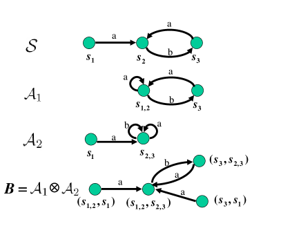
Figure 5: ${\mathcal{S}}$ is the original state space. ${\mathcal{A}}_{1}$ and ${\mathcal{A}}_{2}$ are abstractions of ${\mathcal{S}}$. $B={\mathcal{A}}_{1}\otimes{\mathcal{A}}_{2}$ is the synchronized product of ${\mathcal{A}}_{1}$ and ${\mathcal{A}}_{2}$.

Haslum et al. (?) introduce a family of heuristics, called $h^{m}$ (for any fixed $m\in\{1,2,...\}$), that are based on abstraction, but are not covered by our definition because the value of the heuristic for state $t$, $h^{m}(t)$, is not defined as the distance from the abstraction of $t$ to the abstract goal state. Instead it takes advantage of a special monotonicity property of costs in planning problems: the cost of achieving a subset of the atoms defining the goal is a lower bound on the cost of achieving the goal. When searching backwards from the goal to the start state, as Haslum et al. do, this allows an admissible heuristic to be defined in the following recursive minimax fashion ($|t|$ denotes the number of atoms in state $t$):

$$h^{m}(t)=\left\{\begin{array}[]{ll}0,&t\subseteq start\\ {\displaystyle\min_{(s,t)\in\Pi}}C(s,t)+h^{m}(s),&|t|\leq m\\ {\displaystyle\max_{s\subset t,|s|\leq m}}h^{m}(s),&|t|>m\end{array}\right.$$

The first two lines of this definition are the standard method for calculating the cost of a least-cost path. It is the third line that uses the fact that the cost of achieving any subset of the atoms in $t$ is a lower bound on the cost of achieving the entire set of atoms $t$. The recursive calculation alternates between the min and max calculation depending on the number of atoms in the state currently being considered in the recursive calculation, and is therefore different than a shortest path calculation or taking the maximum of a set of shortest path calculations.

3.4.2 Previous definitions of additive abstractions

Prieditis (?) included a method (“Factor”) in his Absolver II system for creating additive abstractions, but did not present any formal definitions or theory.

The first thorough discussion of additive abstractions is due to Korf and Taylor (?). They observed that the sliding tile puzzle’s Manhattan Distance heuristic, and several of its enhancements, were the sum of the distances in a set of abstract spaces in which a small number of tiles were “distinguished”. As explained in Section 2.1, what allowed the abstract distances to be added and still be a lower bound on distances in the original space is that only the moves of the distinguished tiles counted towards the abstract distance and no tile was distinguished in more than one abstraction. This idea was later developed in a series of papers (?, ?), which extended its application to other domains, such as the 4-peg Towers of Hanoi puzzle.

In the planning literature, the same idea was proposed by Haslum et al. (?), who described it as partitioning the operators into disjoint sets $B_{1},...B_{k}$ and counting the cost of operators in set $B_{i}$ only in abstract space $A_{i}$. The example they give is that in the Blocks World operators that move block $i$ would all be in set $B_{i}$, effectively defining a set of additive abstractions for the Blocks World exactly analogous to the Korf and Taylor abstractions that define Manhattan Distance for the sliding tile puzzle.

Edelkamp (?) took a different approach to defining additive abstractions for STRIPS planning representations. His method involves partitioning the atoms into disjoint sets $V_{1},...V_{k}$ such that no operator changes atoms in more than one group. If abstract space $A_{i}$ retains only the atoms in set $V_{i}$ then the operators that do not affect atoms in $V_{i}$ will have no effect at all in abstract space $A_{i}$ and will naturally have a cost of 0 in $A_{i}$. Since no operator affects atoms in more than one group, no operator has a non-zero cost in more than one abstract space and distances in the abstract spaces can safely be added. Haslum et al. (?) extended this idea to representations in which state variables could have multiple values. In a subsequent paper Edelkamp (?) remarks that if there is no partitioning of atoms that induces a partitioning of the operators as just described, additivity could be “enforced” by assigning an operator a cost of zero in all but one of the abstract spaces—a return to the Korf and Taylor idea.

All the methods just described might be called “all-or-nothing” methods of defining abstract costs, because the cost of each edge $C(\pi)$ is fully assigned as the cost of the corresponding abstract edge $C_{i}(\pi_{i})$ in one of the abstractions and the corresponding edges in all the other abstractions are assigned a cost of zero. Any such method obviously satisfies property (P3) and is therefore additive.

Our theory of additivity does not require abstract methods to be defined in an all-or-nothing manner, it allows $C(\pi)$ to be divided in any way whatsoever among the abstractions as long as property (P3) is satisfied. This possibility has been recognized in one recent publication (?), which did not report any experimental results. This generalization is important because it eliminates the requirement that operators must move only one “tile” or change atoms/variables in one “group”, and the related requirement that tiles/atoms be distinguished/represented in exactly one of the abstract spaces. This requirement restricted the application of previous methods for defining additive abstractions, precluding their application to state spaces such as Rubik’s Cube, the Pancake puzzle, and TopSpin. As the following sections show, with our definition, additive abstractions can be defined for any state space, including the three just mentioned.

Finally, Helmert et al. (?) showed that the synchronized product of additive abstractions produces a heuristic $h_{sprod}$ that dominates $h_{add}$, in the sense that $h_{sprod}(s)\geq h_{add}(s)$ for all states $s$. This happens because the synchronized product forces the same path to be used in all the abstract spaces, whereas the calculation of each $C^{*}_{i}$ in $h_{add}$ can be based on a different path. The discussion of the negative results and infeasibility below highlight the problems that can arise because each $C^{*}_{i}$ is calculated independently.

4 New Applications of Additive Abstractions

This section and the next section report the results of applying the general definition of additive abstraction given in the previous section to three benchmark state spaces: TopSpin, the Pancake puzzle and Rubik’s Cube. A few additional experimental results may be found in the previous paper by ? (?). In all our experiments all edges in the original state spaces have a cost of 1 and we define $R_{i}(\pi_{i})=1-C_{i}(\pi_{i})$, its maximum permitted value when edges cost 1. We use pattern databases to store the heuristic values. The pre-processing time required to compute the pattern databases is excluded from the times reported in the results, because the PDB needs to be calculated only once and this overhead is amortized over the solving of many problem instances.

4.1 Methods for Defining Costs

We will investigate two general methods for defining the primary cost of an abstract state transition $C_{i}(\pi_{i})$, which we call “cost-splitting” and “location-based” costs. To illustrate the generality of these methods we will define them for the two most common ways of representing states—as a vector of state variables, which is the method we implemented in our experiments, and as a set of logical atoms as in the STRIPS representation for planning problems.

In a state variable representation a state $t$ is represented by a vector of $m$ state variables, each having its own domain of possible values $D_{j}$, i.e., $t=(t(0),...,t(m-1))$, where $t(j)\in D_{j}$ is the value assigned to the $j^{th}$ state variable in state $t$. For example, in puzzles such as the Pancake puzzle and the sliding tile puzzles, there is typically one variable for each physical location in the puzzle, and the value of $t(j)$ indicates which “tile” is in location $j$ in state $t$. In this case the domain for all the variables is the same. State space abstractions are defined by abstracting the domains. In particular, in this setting domain abstraction $\psi_{i}$ will leave specific domain values unchanged (the “distinguished” values according to $\psi_{i}$) and map all the rest to the same special value, “don’t care”. The abstract state corresponding to $t$ according to $\psi_{i}$ is $t_{i}$=$(t_{i}(0),...,t_{i}(m-1))$ with $t_{i}(j)=\psi_{i}(t(j))$. As in previous research with these state spaces a set of abstractions is defined by partitioning the domain values into disjoint sets $E_{1},...,E_{k}$ with $E_{i}$ being the set of distinguished values in abstraction $i$. Note that the theory developed in the previous section does not require the distinguished values in different abstractions to be mutually exclusive; it allows a value to be distinguished in any number of abstract spaces provided abstract costs are defined appropriately.

As mentioned previously, in a STRIPS representation a state is represented by the set of logical atoms that are true in the state. A state variable representation can be converted to a STRIPS representation in a variety of ways, the simplest being to define an atom for each possible variable-value combination. If state variable $j$ has value $v$ in the state variable representation of state $t$ then the atom $variable$-$j$-$has$-$value$-$v$ is true in the STRIPS representation of $t$. The exact equivalent of domain abstraction can be achieved by defining $V_{i}$, the set of atoms to be used in abstraction $i$, to be all the atoms $variable$-$j$-$has$-$value$-$v$ in which $v\in E_{i}$, the set of distinguished values for domain abstraction $i$.

4.1.1 Cost-splitting

In a state variable representation, the cost-splitting method of defining primary costs works as follows. A state transition $\pi$ that changes $b^{\pi}$ state variables has its cost, $C(\pi)$, split among the corresponding abstract state transitions $\pi_{1},\dots,\pi_{k}$ in proportion to the number of distinguished values they assign to the variables, i.e., in abstraction $i$

$$C_{i}(\pi_{i})=\frac{b^{\pi}_{i}*C(\pi)}{b^{\pi}}$$

if $\pi$ changes $b^{\pi}$ variables and $b^{\pi}_{i}$ of them are assigned distinguished values by $\pi_{i}$. For example, the $3\times 3\times 3$ Rubik’s cube is composed of twenty little moveable “cubies” and each operator moves eight cubies, four corner cubies and four edge cubies. Hence $b^{\pi}=8$ for all state transitions $\pi$. If a particular state transition moves three cubies that are distinguished according to abstraction $\psi_{i}$, the corresponding abstract state transition, $\pi_{i}$, would cost $\frac{3}{8}$. Strictly speaking, we require abstract edge costs to be integers, so the fractional edge costs produced by cost-splitting must be scaled appropriately to become integers. Our implementation of cost-splitting actually does this scaling but it will simplify our presentation of cost-splitting to talk of the edge costs as if they were fractional.

If each domain value is distinguished in at most one abstraction (e.g. if the abstractions are defined by partitioning the domain values) cost-splitting produces additive abstractions, i.e., $C(\pi)\geq\sum_{i=1}^{k}C_{i}(\pi_{i})$ for all $\pi\in\Pi$. Because $C(\pi)$ is known to be an integer, $h_{add}$ can be defined to be the ceiling of the sum of the abstract distances, $\lceil\hskip 2.84544pt\sum_{i=1}^{k}C_{i}(\pi_{i})\rceil$, instead of just the sum.

With a STRIPS representation, cost-splitting could be defined identically, with $b^{\pi}$ being the number of atoms changed (added or deleted) by operator $\pi$ in the original space and $b^{\pi}_{i}$ being the number of atoms changed by the corresponding operator in abstraction $i$.

4.1.2 Location-based Costs

In a location-based cost definition for a state variable representation, a state variable $loc_{\pi}$ is associated with state transition $\pi$ and $\pi$’s full cost $C(\pi)$ is assigned to abstract state transition $\pi_{i}$ if $\pi_{i}$ changes the value of variable $loc_{\pi}$ to a value that is distinguished according to $\psi_{i}$. Formally:

$$C_{i}(\pi_{i})=\left\{\begin{array}[]{ll}C(\pi),&\mbox{if $\pi_{i}=(t^{1}_{i},t^{2}_{i})$, $t^{1}_{i}(loc^{\pi})\neq t^{2}_{i}(loc^{\pi})$, and}\\ &\mbox{$t^{2}_{i}(loc^{\pi})$ is a distinguished value according to $\psi_{i}$.}\\ 0,&\mbox{otherwise.}\end{array}\right.$$

Instead of focusing on the value that is assigned to variable $loc_{\pi}$, location-based costs can be defined equally well on the value that variable $loc_{\pi}$ had before it was changed. In either case, if each domain value is distinguished in at most one abstraction location-based costs produce additive abstractions. The name “location-based” is based on the typical representations used for puzzles, in which there is a state variable for each physical location in the puzzle. For example, in Rubik’s Cube one could choose the reference variables to be the ones representing the two diagonally opposite corner locations in the puzzle. Note that each possible Rubik’s cube operator changes exactly one of these locations. An abstract state transition would have a primary cost of 1 if the cubie it moved into one of these locations was a distinguished cubie in its abstraction, and a primary cost of 0 otherwise.

For a STRIPS representation of states, location-based costs can be defined by choosing an atom $a$ in the $Add$ list for each operator $\pi$ and assigning the full cost $C(\pi)$ to abstraction $i$ if $a$ appears in the $Add$ list of $\pi_{i}$. If atoms are partitioned so that each atom appears in at most one abstraction, this method will define additive costs.

Although the cost-splitting and location-based methods for defining costs can be applied to a wide range of state spaces, they are not guaranteed to define heuristics that are superior to other heuristics for a given state space. We determined experimentally that heuristics based on cost-splitting substantially improve performance for sufficiently large versions of TopSpin and that heuristics based on location-based costs vastly improve the state of the art for the 17-Pancake puzzle. In our experiments additive heuristics did not improve the state of the art for Rubik’s Cube. The following subsections describe the positive results in detail. The negative results are discussed in Section 5.

4.2 TopSpin with Cost-Splitting

In the $(N,K)$-TopSpin puzzle (see Figure 6) there are $N$ tiles (numbered $1,\dots,N$) arranged on a circular track, and two physical movements are possible: (1) the entire set of tiles may be rotated around the track, and (2) a segment consisting of $K$ adjacent tiles in the track may be reversed. As in previous formulations of this puzzle as a state space (?, ?, ?), we do not represent the first physical movement as an operator, but instead designate one of the tiles (tile 1) as a reference tile with the goal being to get the other tiles in increasing order starting from this tile (regardless of its position). The state space therefore has $N$ operators (numbered $1,\dots,N$), with operator $a$ reversing the segment of length $K$ starting at position $a$ relative to the current position of tile 1. For certain combinations of $N$ and $K$ all possible permutations can be generated from the standard goal state by these operators, but in general the space consists of connected components and so not all states are reachable (?). In the experiments in this section, $K=4$ and $N$ is varied.

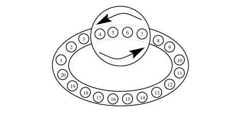
Figure 6: The TopSpin puzzle.

The sets of abstractions used in these experiments are described using a tuple written as $a_{1}$–$a_{2}$–$\dots$–$a_{M}$, indicating that the set contains $M$ abstractions, with tiles $1\dots(a_{1})$ distinguished in the first abstraction, tiles $(a_{1}+1)\dots(a_{1}+a_{2})$ distinguished in the second abstraction, and so on. For example, 6-6-6 denotes a set of three abstractions in which the distinguished tiles are ($1\dots 6$), ($7\dots 12$), and ($13\dots 18$) respectively.

The experiments compare $h_{add}$, the additive use of a set of abstractions, with $h_{max}$, the standard use of the same abstractions, in which, as described in Section 2, the full cost of each state transition is counted in each abstraction and the heuristic returns the maximum distance to goal returned by the different abstractions. Cost-splitting is used to define operator costs in the abstract spaces for $h_{add}$. Because $K=4$, each operator moves 4 tiles. If $b_{i}$ of these are distinguished tiles when operator $op$ is applied to state $s_{i}$ in abstraction $i$, applying $op$ to $s_{i}$ has a primary cost of $\frac{b_{i}}{4}$ in abstraction $i$.

In these experiments the heuristic defined by each abstraction is stored in a pattern database (PDB). Each abstraction would normally be used to define its own PDB, so that a set of $M$ abstractions would require $M$ PDBs. However, for TopSpin, if two (or more) abstractions have the same number of distinguished tiles and the distinguished tiles are all adjacent, one PDB can be used for all of them by suitably renaming the tiles before doing the PDB lookup. For the 6-6-6 abstractions, for example, only one PDB is needed, but three lookups would be done in it, one for each abstraction. Because the position of tile 1 is effectively fixed, this PDB is $N$ times smaller than it would normally be. For example, with $N=18$, the PDB for the 6-6-6 abstractions contains $17\times 16\times\ldots\times 13$ entries. The memory needed for each entry in the $h_{add}$ PDBs is twice the memory needed for an entry in the $h_{max}$ PDBs because of the need to represent fractional values.

We ran experiments for the values of $N$ and sets of abstractions shown in the first two columns of Table 1. Start states were generated by a random walk of 150 moves from the goal state. There were 1000, 50 and 20 start states for $N=12,16$ and $18$, respectively. The average solution length for these start states is shown in the third column of Table 1. The average number of nodes generated and the average CPU time (in seconds) for $\textit{IDA}^{*}$ to solve the given start states is shown in the Nodes and Time columns for each of $h_{max}$ and $h_{add}$. The Nodes Ratio column gives the ratio of Nodes using $h_{add}$ to Nodes using $h_{max}$. A ratio less than one (highlighted in bold) indicates that $h_{add}$, the heuristic based on additive abstractions with cost-splitting, is superior to $h_{max}$, the standard heuristic using the same set of abstractions.

		Average			$h_{add}$ based on
$N$	Abs	Solution	$h_{max}$		cost-splitting		Nodes
		Length	Nodes	Time	Nodes	Time	Ratio
12	6-6	9.138	14,821	0.05	53,460	0.16	3.60
12	4-4-4	9.138	269,974	1.10	346,446	1.33	1.28
12	3-3-3-3	9.138	1,762,262	8.16	1,388,183	6.44	0.78
16	8-8	14.040	1,361,042	3.42	2,137,740	4.74	1.57
16	4-4-4-4	14.040	4,494,414,929	13,575.00	251,946,069	851.00	0.056
18	9-9	17.000	38,646,344	165.42	21,285,298	91.76	0.55
18	6-6-6	17.000	18,438,031,512	108,155.00	879,249,695	4,713.00	0.04

Table 1: ($N,4$)-TopSpin results using cost-splitting.

When $N=12$ and $N=16$ the best performance is achieved by $h_{max}$ based on a pair of abstractions each having $\frac{N}{2}$ distinguished tiles. As $N$ increases the advantage of $h_{max}$ decreases and, when $N=18$, $h_{add}$ outperforms $h_{max}$ for all abstractions used. Moreover, even for the smaller values of $N$ $h_{add}$ outperforms $h_{max}$ when a set of four abstractions with $\frac{N}{4}$ distinguished tiles each is used. This is important because as $N$ increases, memory limitations will preclude using abstractions with $\frac{N}{2}$ distinguished tiles and the only option will be to use more abstractions with fewer distinguished tiles each. The results in Table 1 show that $h_{add}$ will be the method of choice in this situation.

4.3 The Pancake Puzzle with Location-based Costs

In this section, we present the experimental results on the 17-Pancake puzzle using location-based costs. The same notation as in the previous section is used to denote sets of abstractions, e.g. 5-6-6 denotes a set of three abstractions, with the first having tiles ($0\dots 4$) as its distinguished tiles, the second having tiles ($5\dots 10$) as its distinguished tiles, and the third having tiles ($11\dots 16$) as its distinguished tiles. Also as before, the heuristic for each abstraction is precomputed and stored in a pattern database (PDB). Unlike TopSpin, there are no symmetries in the Pancake puzzle that enable different abstractions to make use of the same PDB, so a set of $M$ abstractions for the Pancake puzzle requires $M$ different PDBs.

Additive abstractions are defined using the location-based method with just one reference location, the leftmost position. This position was chosen because the tile in this position changes whenever any operator is applied to any state in the original state space. This means that every edge cost in the original space will be fully counted in some abstract space as long as each tile is a distinguished tile in some abstraction. As before, we use $h_{add}$ to denote the heuristic defined by adding the values returned by the individual additive abstractions.

Our first experiment compares $\textit{IDA}^{*}$ using $h_{add}$ with the best results known for the 17-Pancake puzzle (?) (shown in Table 2), which were obtained using a single abstraction having the rightmost seven tiles (10–16) as its distinguished tiles and an advanced search technique called Dual $\textit{IDA}^{*}$ ($\textit{DIDA}^{*}$). $\textit{DIDA}^{*}$ is an extension of $\textit{IDA}^{*}$ that exploits the fact that, when states are permutations of tiles as in the Pancake puzzle, each state $s$ has an easily computable “dual state” $s^{d}$ with the special property that inverses of paths from $s$ to the goal are paths from $s^{d}$ to the goal. If paths and their inverses cost the same, $\textit{DIDA}^{*}$ defines the heuristic value for state $s$ as the maximum of $h(s)$ and $h(s^{d})$, and sometimes will decide to search for a least-cost path from $s^{d}$ to goal when it is looking for a path from $s$ to goal.

The results of this experiment are shown in the top three rows of Table 3. The Algorithm column indicates the heuristic search algorithm. The Abs column shows the set of abstractions used to generate heuristics. The Nodes column shows the average number of nodes generated in solving 1000 randomly generated start states. These start states have an average solution length of 15.77. The Time column gives the average number of CPU seconds needed to solve these start states on an AMD Athlon(tm) 64 Processor 3700+ with 2.4 GHz clock rate and 1GB memory. The Memory column indicates the total size of each set of PDBs.

			Average	$h$ based on
$N$	Algorithm	Abs	Solution	a single large PDB
			Length	Nodes	Time	Memory
17	$\textit{DIDA}^{*}$	rightmost-7	15.77	124,198,462	37.713	98,017,920

Table 2: The best results known for the 17-Pancake puzzle (?), which were obtained using a single abstraction having the rightmost seven tiles ($10-16$) as its distinguished tiles and an advanced search technique called Dual $\textit{IDA}^{*}$ ($\textit{DIDA}^{*}$).

			Average	$h_{add}$ based on
$N$	Algorithm	Abs	Solution	Location-based Costs
			Length	Nodes	Time	Memory
17	$\textit{IDA}^{*}$	4-4-4-5	15.77	14,610,039	4.302	913,920
17	$\textit{IDA}^{*}$	5-6-6	15.77	1,064,108	0.342	18,564,000
17	$\textit{IDA}^{*}$	3-7-7	15.77	1,061,383	0.383	196,039,920
17	$\textit{DIDA}^{*}$	4-4-4-5	15.77	368,925	0.195	913,920
17	$\textit{DIDA}^{*}$	5-6-6	15.77	44,618	0.028	18,564,000
17	$\textit{DIDA}^{*}$	3-7-7	15.77	37,155	0.026	196,039,920

Table 3: 17-Pancake puzzle results using $h_{add}$ based on location-based costs.

Clearly, the use of $h_{add}$ based on location-based costs results in a very significant reduction in nodes generated compared to using a single large PDB, even when the latter has the advantage of being used by a more sophisticated search algorithm. Note that the total memory needed for the 4-4-4-5 PDBs is only one percent of the memory needed for the rightmost-7 PDB, and yet $\textit{IDA}^{*}$ with 4-4-4-5 generates 8.5 times fewer nodes than $\textit{DIDA}^{*}$with the rightmost-7 PDB. Getting excellent search performance from a very small PDB is especially important in situations where the cost of computing the PDBs must be taken into account in addition to the cost of problem-solving (?).

The memory requirements increase significantly when abstractions contain more distinguished tiles, but in this experiment the improvement of the running time does not increase accordingly. For example, the 3-7-7 PDBs use ten times more memory than the 5-6-6 PDBs, but the running time is almost the same. This is because the 5-6-6 PDBs are so accurate there is little room to improve them. The average heuristic value on the start states using the 5-6-6 PDBs is 13.594, only 2.2 less than the actual average solution length. The average heuristic value using the 3-7-7 PDBs is only slightly higher (13.628).

The last three rows in Table 3 show the results when $h_{add}$ with location-based costs is used in conjunction with $\textit{DIDA}^{*}$. These results show that combining our additive abstractions with state-of-the-art search techniques results in further significant reductions in nodes generated and CPU time. For example, the 5-6-6 PDBs use only 1/5 of the memory of the rightmost-7 PDB but reduce the number of nodes generated by $\textit{DIDA}^{*}$ by a factor of 2783 and the CPU time by a factor of 1347.

To compare $h_{add}$ to $h_{max}$ we ran plain $\textit{IDA}^{*}$ with $h_{max}$ on the same 1000 start states, with a time limit for each start state ten times greater than the time needed to solve the start state using $h_{add}$. With this time limit only 63 of the 1000 start states could be solved with $h_{max}$ using the 3-7-7 abstraction, only 5 could be solved with $h_{max}$ using the 5-6-6 abstraction, and only 3 could be solved with $h_{max}$ using the 4-4-4-5 abstraction. To determine if $h_{add}$’s superiority over $h_{max}$ for location-based costs on this puzzle could have been predicted using Lemma 3.6, we generated 100 million random 17-Pancake puzzle states and tested how many satisfied the requirements of Lemma 3.6. Over 98% of the states satisfied those requirements for the 3-7-7 abstraction, and over 99.8% of the states satisfied its requirements for the 5-6-6 and 4-4-4-5 abstractions.

5 Negative Results

Not all of our experiments yielded positive results. Here we explore some trials where our additive approaches did not perform as well. By examining some of these cases closely, we shed light on the conditions which might indicate when these approaches will be useful.

5.1 TopSpin with Location-Based Costs

In this experiment, we used the 6-6-6 abstraction of $(18,4)$-TopSpin as in Section 4.2 but with location-based costs instead of cost-splitting. The primary cost of operator $a$, the operator that reverses the segment consisting of locations $a$ to $a+3$ ($modulo$ $18$), is $1$ in abstract space $i$ if the tile in location $a$ before the operator is applied is distinguished according to abstraction $\psi_{i}$ and $0$ otherwise.

This definition of costs was disastrous, resulting in $C^{*}_{i}(t_{i},g_{i})=0$ for all abstract states in all abstractions. In other words, in finding a least-cost path it was never necessary to use operator $a$ when there was a distinguished tile in location $a$. It was always possible to move towards the goal by applying another operator, $a^{\prime}$, with a primary cost of $0$. To illustrate how this is possible, consider state 0 4 5 6 3 2 1 of $(7,4)$-$TopSpin$. This state can be transformed into the goal in a single move: the operator that reverses the four tiles starting with tile $3$ produces the state 3 4 5 6 0 1 2 which is equal to the goal state when it is cyclically shifted to put $0$ into the leftmost position. With the 4-3 abstraction this move has a primary cost of $0$ in the abstract space based on tiles $4...6$, but it would have a primary cost of $1$ in the abstract space based on tiles $0...3$ (because tile $3$ is in the leftmost location changed by the operator). However the following sequence maps tiles $0...3$ to their goal locations and has a primary cost of $0$ in this abstract space (because a “don’t care” tile is always moved from the reference location):

0

*

*

*

3

2

1

0

*

*

1

2

3

*

0

*

3

2

1

*

*

0

1

2

3

*

*

*

5.2 Rubik’s Cube

The success of cost-splitting on (18,4)-TopSpin suggested it might also provide an improved heuristic for Rubik’s Cube, which can be viewed as a 3-dimensional version of (20,8)-TopSpin. We used the standard method of partitioning the cubies to create three abstractions, one based on the 8 corner cubies, and the others based on 6 edge cubies each. The standard heuristic based on this partitioning, $h_{max}$, expanded approximately three times fewer nodes than $h_{add}$ based on this partitioning and primary costs defined by cost-splitting. The result was similar whether the 24 symmetries of Rubik’s Cube were used to define multiple heuristic lookups or not.

We believe the reason for cost-splitting working well for (18,4)-TopSpin but not Rubik’s Cube is that an operator in Rubik’s Cube moves more cubies than the number of tiles moved by an operator in (18,4)-TopSpin. To test if operators moving more tiles reduces the effectiveness of cost-splitting we solved 1000 instances of (12,$K$)-TopSpin for various values of $K$, all using the 3-3-3-3 abstraction. The results are shown in Table 4. The Nodes Ratio column gives the ratio of Nodes using $h_{add}$ to Nodes using $h_{max}$. A ratio less than one (highlighted in bold) indicates that $h_{add}$ is superior to $h_{max}$. The results clearly show that $h_{add}$ based on cost-splitting is superior to $h_{max}$ for small $K$ and steadily loses its advantage as $K$ increases. The same phenomenon can also be seen in Table 1, where increasing $N$ relative to $K$ increases the effectiveness of additive heuristics based on cost-splitting.

			$h_{add}$ based on
$K$	$h_{max}$		cost-splitting		Nodes
	Nodes	Time	Nodes	Time	Ratio
3	486,515	2.206	207,479	0.952	0.42
4	1,762,262	8.164	1,388,183	6.437	0.78
5	8,978	0.043	20,096	0.095	2.23
6	193,335,181	901.000	2,459,204,715	11,457.000	12.72

Table 4: ($12,K$)-TopSpin results using cost-splitting.

We also investigated location-based costs for Rubik’s Cube. The cubies were partitioned into four groups, each containing three edge cubies and two corner cubies, and an abstraction was defined using each group. Two diagonally opposite corner positions were used as the reference locations (as noted above, each Rubik’s Cube operator changes exactly one of these locations). The resulting $h_{add}$ heuristic was so weak we could not solve random instances of the puzzle with it.

5.3 The Pancake Puzzle with Cost-Splitting

Table 5 compares $h_{add}$ and $h_{max}$ on the 13-Pancake puzzle when costs are defined using cost-splitting. The memory is greater for $h_{add}$ than $h_{max}$ because the fractional entries that cost-splitting produces require more bits per entry than the small integer values stored in the $h_{max}$ PDB. In terms of both run-time and number of nodes generated, $h_{add}$ is inferior to $h_{max}$ for these costs, the opposite of what was seen in Section 4.3 using location-based costs.

		Average			$h_{add}$ based on
$N$	Abs	Solution	$h_{max}$		costing-splitting
		Length	Nodes	Time	Nodes	Time
13	6-7	11.791	166,479	0.0466	1,218,903	0.3622

Table 5: $h_{add}$ vs. $h_{max}$ on the 13-Pancake puzzle.

Cost-splitting, as we have defined it for the Pancake puzzle, adversely affects $h_{add}$ because it enables each individual abstraction to get artificially low estimates of the cost of solving its distinguished tiles by increasing the number of “don’t care” tiles that are moved. For example, with cost-splitting the least-cost sequence of operators to get tile “0” into its goal position from abstract state * 0 * * * is not the obvious single move of reversing the first two positions. That move costs $\frac{1}{2}$, whereas the 2-move sequence that reverses the entire state and then reverses the first four positions costs only $\frac{1}{5}+\frac{1}{4}$.

As a specific example, consider state 7 4 5 6 3 8 0 10 9 2 1 11 of the 12-Pancake puzzle. Using the 6-6 abstractions, the minimum number of moves to get tiles 0–5 into their goal positions is 8, and for 6–11 it is 7, where in each case we ignore the final locations of the other tiles. Thus, $h_{max}$ is 8. By contrast, $h_{add}$ is $6.918$, which is less than even the smaller of the two numbers used to define $h_{max}$. The two move sequences whose costs are added to compute $h_{add}$ for this state each have slightly more moves than the corresponding sequences on which $h_{max}$ is based (10 and 9 compared to 8 and 7), but involve more than twice as many “don’t care” tiles (45 and 44 compared to 11 and 17) and so are less costly.

There is hope that this pathological situation can be detected, at least sometimes, by inspecting the residual costs. If the residual costs are defined to be complementary to the primary costs (i.e. $R_{i}(\pi_{i})=C(\pi)-C_{i}(\pi_{i})$), as we have done, then decreasing the primary cost increases the residual cost. If the residual cost is sufficiently large in one of the abstract spaces the conditions of Lemma 3.10 will be satisfied, signalling that the value returned by $h_{add}$ is provably too low. This is the subject of the next section, on “infeasibility”.

6 Infeasible Heuristic Values

This section describes a way to increase the heuristic values defined by additive abstractions in some circumstances. The key to the approach is to identify “infeasible” values—ones that cannot possibly be the optimal solution cost. Once identified the infeasible values can be increased to give a better estimate of the solution cost. An example of infeasibility occurs with the Manhattan Distance (MD) heuristic for the sliding tile puzzle. It is well-known that the parity of $\textit{MD}(t)$ is the same as the parity of the optimal solution cost for state $t$. If some other heuristic for the sliding tile puzzle returns a value of the opposite parity, it can safely be increased until it has the correct parity. This example relies on specific properties of the MD heuristic and the puzzle. Lemma 3.10 gives a problem-independent method for testing infeasibility, and that is what we will use.

To illustrate how infeasibility can be detected using Lemma 3.10 consider the example in Figure 3. The solution to the abstract problem shown in the middle part of the figure requires 9 distinguished moves, so $C^{*}_{1}(A_{1})=9$. The abstract paths that solve the problem with 9 distinguished moves require, at a minimum, 9 “don’t care” moves, so $R^{*}_{1}(A_{1})=9$. A similar calculation for the abstract space on the right of the figure yields $C^{*}_{2}(A_{2})=5$ and $R^{*}_{2}(A_{2})=7$. The value of $h_{add}(A,g)$ is therefore $C^{*}_{1}(A_{1})+C^{*}_{2}(A_{2})=9+5=14$. This value is based on the assumption that there is a path in the original space that makes $C^{*}_{1}(A_{1})=9$ moves of tiles 1, 3, 5, and 7, and $C^{*}_{2}(A_{2})=5$ moves of the other tiles. However, the value of $R^{*}_{1}(A_{1})$ tells us that any path that uses only $9$ moves of tiles 1, 3, 5, and 7 to put them into their goal locations must make at least $9$ moves of the other tiles, it cannot possibly make just $5$ moves. Therefore there does not exist a solution costing as little as $C^{*}_{1}(A_{1})+C^{*}_{2}(A_{2})=14$.

To illustrate the potential of this method for improving additive heuristics, Table 6 shows the average results of $\textit{IDA}^{*}$ solving 1000 test instances of the 15-puzzle using two different tile partitionings (shown in Figure 7) and costs defined by the method described in Section 2.1. These additive heuristics have the same parity property as Manhattan Distance, so when infeasibility is detected $2$ can be added to the value. The $h_{add}$ columns show the average heuristic value of the 1000 start states. As can be seen infeasibility checking increases the initial heuristic value by over 0.5 and reduces the number of nodes generated and the CPU time by over a factor of $2$. However, there is a space penalty for this improvement, because the $R^{*}$ values must be stored in the pattern database in addition to the normal $C^{*}$ values. This doubles the amount of memory required, and it is not clear if storing $R^{*}$ is the best way to use this extra memory. This experiment merely shows that infeasibility checking is one way to use extra memory to speed up search for some problems.

         

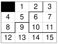
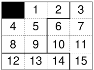
Figure 7: Different tile partitionings for the 15-puzzle (left: 5-5-5; right: 6-6-3).

		Average	$h_{add}$ based on zero-one cost-splitting
$N$	Abs	Solution	No Infeasibility Check			Infeasibility Check
		Length	$h_{add}$	Nodes	Time	$h_{add}$	Nodes	Time
15	5-5-5	52.522	41.56	3,186,654	0.642	42.10	1,453,358	0.312
15	6-6-3	52.522	42.13	1,858,899	0.379	42.78	784,145	0.171

Table 6: The effect of infeasibility checking on the 15-puzzle.

Slightly stronger results were obtained for the $(N,4)$-TopSpin puzzle with costs defined by cost-splitting, as described in Section 4.2. The “No Infeasibility Check” columns in Table 7 are the same as the “$h_{add}$ based on cost-splitting” columns of the corresponding rows in Table 1. Comparing these to the “Infeasibility Check” columns shows that in most cases infeasibility checking reduces the number of nodes generated and the CPU time by roughly a factor of 2.

When location-based costs are used with TopSpin infeasibility checking adds one to the heuristic value of almost every state. However, this simply means that most states have a heuristic value of 1 instead of 0 (recall the discussion in Section 5.1), which is still a very poor heuristic.

		Average	$h_{add}$ based on costing-splitting
$N$	Abs	Solution	No Infeasibility Check		Infeasibility Check
		Length	Nodes	Time	Nodes	Time
12	6-6	9.138	53,460	0.16	20,229	0.07
12	4-4-4	9.138	346,446	1.33	174,293	0.62
12	3-3-3-3	9.138	1,388,183	6.44	1,078,853	4.90
16	8-8	14.040	2,137,740	4.74	705,790	1.80
16	4-4-4-4	14.040	251,946,069	851.00	203,213,736	772.04
18	6-6-6	17.000	879,249,695	4,713.00	508,851,444	2,846.52

Table 7: The effect of infeasibility checking on ($N,4$)-TopSpin using cost-splitting.

Infeasibility checking produces almost no benefit for the 17-Pancake puzzle with location-based costs because the conditions of Lemma 3.10 are almost never satisfied. The experiment discussed at the end of Section 4.3 showed that fewer than 2% of the states satisfy the conditions of Lemma 3.10 for the 3-7-7 abstraction, and fewer than 0.2% of the states satisfy the conditions of Lemma 3.10 for the 5-6-6 and 4-4-4-5 abstractions.

Infeasibility checking for the 13-Pancake puzzle with cost-splitting also produces very little benefit, but for a different reason. For example, Table 8 shows the effect of infeasibility checking on the 13-Pancake puzzle; the results shown are averages over 1000 start states. Cost-splitting in this state space produces fractional edge costs that are multiples of $\frac{1}{360360}$ (360360 is the Least Common Multiple of the integers from 1 to 13), and therefore if infeasibility is detected the amount added is $\frac{1}{360360}$. But recall that $h_{add}$, with cost-splitting, is defined as the ceiling of $\sum_{i=1}^{k}C_{i}(\pi_{i})$. The value of $h_{add}$ will therefore be the same, whether $\frac{1}{360360}$ is added or not, unless the sum of the $C_{i}(\pi_{i})$ is exactly an integer. As Table 8 shows, this does happen but only rarely.

		Average	$h_{add}$ based on costing-splitting
$N$	Abs	Solution	No Infeasibility Check		Infeasibility Check
		Length	Nodes	Time	Nodes	Time
13	6-7	11.791	1,218,903	0.3622	1,218,789	0.4453

Table 8: The effect of infeasibility checking on the 13-Pancake puzzle using cost-splitting.

7 Conclusions

In this paper we have presented a formal, general definition of additive abstractions that removes the restrictions of most previous definitions, thereby enabling additive abstractions to be defined for any state space. We have proven that heuristics based on additive abstractions are consistent as well as admissible. Our definition formalizes the intuitive idea that abstractions will be additive provided the cost of each operator is divided among the abstract spaces, and we have presented two specific, practical methods for defining abstract costs, cost-splitting and location-based costs. These methods were applied to three standard state spaces that did not have additive abstractions according to previous definitions: TopSpin, Rubik’s Cube, and the Pancake puzzle. Additive abstractions using cost-splitting reduce search time substantially for (18,4)-TopSpin and additive abstractions using location-based costs reduce search time for the 17-Pancake puzzle by three orders of magnitude over the state of the art. We also report negative results, for example on Rubik’s Cube, demonstrating that additive abstractions are not always superior to the standard, maximum-based method for combining multiple abstractions.

A distinctive feature of our definition is that each edge in an abstract space has two costs instead of just one. This was inspired by previous definitions treating “distinguished” moves differently than “don’t care” moves in calculating least-cost abstract paths. Formalizing this idea with two costs per edge has enabled us to develop a way of testing if the heuristic value returned by additive abstractions is provably too low (“infeasible”). This test produced no speedup when applied to the Pancake puzzle, but roughly halved the search time for the 15-puzzle and in most of our experiments with TopSpin.

8 Acknowledgments

This research was supported in part by funding from Canada’s Natural Sciences and Engineering Research Council (NSERC). Sandra Zilles and Jonathan Schaeffer suggested useful improvements to drafts of this paper. This research was also supported by the Israel Science Foundation (ISF) under grant number 728/06 to Ariel Felner.

References

- Banerji Banerji, R. B. (1980). Artificial Intelligence: A Theoretical Approach. North Holland.
- Chen and Skiena Chen, T., and Skiena, S. (1996). Sorting with fixed-length reversals. Discrete Applied Mathematics, 71(1–3), 269–295.
- Culberson and Schaeffer Culberson, J. C., and Schaeffer, J. (1996). Searching with pattern databases. In Advances in Artificial Intelligence (Lecture Notes in Artificial Intelligence 1081), pp. 402–416. Springer.
- Culberson and Schaeffer Culberson, J. C., and Schaeffer, J. (1994). Efficiently searching the 15-puzzle. Tech. rep. TR94-08, Department of Computing Science, University of Alberta.
- Culberson and Schaeffer Culberson, J. C., and Schaeffer, J. (1998). Pattern databases. Computational Intelligence, 14(3), 318–334.
- Edelkamp Edelkamp, S. (2001). Planning with pattern databases. In Proceedings of the 6th European Conference on Planning, pp. 13–24.
- Edelkamp Edelkamp, S. (2002). Symbolic pattern databases in heuristic search planning. In Proceedings of Sixth International Conference on AI Planning and Scheduling (AIPS-02), pp. 274–283.
- Erdem and Tillier Erdem, E., and Tillier, E. (2005). Genome rearrangement and planning. In Proceedings of the Twentieth National Conference on Artificial Intelligence (AAAI-05), pp. 1139–1144.
- Felner and Adler Felner, A., and Adler, A. (2005). Solving the 24 puzzle with instance dependent pattern databases. Proc. SARA-2005, Lecture Notes in Artificial Intelligence, 3607, 248–260.
- Felner et al. Felner, A., Korf, E., and Hanan, S. (2004). Additive pattern database heuristics. Journal of Artificial Intelligence Research, 22, 279–318.
- Felner et al. Felner, A., Zahavi, U., Schaeffer, J., and Holte, R. (2005). Dual lookups in pattern databases. In Proceedings of the Nineteenth International Joint Conference on Artificial Intelligence (IJCAI-05), pp. 103–108.
- Gaschnig Gaschnig, J. (1979). A problem similarity approach to devising heuristics: First results. In Proceedings of the Sixth International Joint Conference on Artificial Intelligence (IJCAI-79), pp. 301–307.
- Guida and Somalvico Guida, G., and Somalvico, M. (1979). A method for computing heuristics in problem solving. Information Sciences, 19, 251–259.
- Haslum et al. Haslum, P., Bonet, B., and Geffner, H. (2005). New admissible heurisitics for domain-independent planning. In Proceedings of The Twentieth National Conference on Artificial Intelligence (AAAI-05), pp. 1163–1168.
- Haslum et al. Haslum, P., Botea, A., Helmert, M., Bonet, B., and Koenig, S. (2007). Domain-independent construction of pattern database heuristics for cost-optimal planning. In Proceedings of The Twenty-Second National Conference on Artificial Intelligence (AAAI-07), pp. 1007–1012.
- Hell and Nesetril Hell, P., and Nesetril, J. (2004). Graphs and homomorphisms. The Oxford Lecture Series in Mathematics and its Applications, 28.
- Helmert et al. Helmert, M., Haslum, P., and Hoffmann, J. (2007). Flexible abstraction heuristics for optimal sequential planning. In Proceedings of the 17th International Conference on Automated Planning and Scheduling (ICAPS-07), pp. 176–183.
- Hernádvölgyi and Holte Hernádvölgyi, I., and Holte, R. C. (2000). Experiments with automatically created memory-based heuristics. Proc. SARA-2000, Lecture Notes in Artificial Intelligence, 1864, 281–290.
- Hernádvölgyi Hernádvölgyi, I. T. (2003). Solving the sequential ordering problem with automatically generated lower bounds. In Proceedings of Operations Research 2003 (Heidelberg, Germany), pp. 355–362.
- Holte et al. Holte, R. C., Perez, M. B., Zimmer, R. M., and MacDonald, A. J. (1996). Hierarchical A*: Searching abstraction hierarchies efficiently. In Proceedings of the Thirteenth National Conference on Artificial Intelligence (AAAI-96), pp. 530–535.
- Holte et al. Holte, R. C., Felner, A., Newton, J., Meshulam, R., and Furcy, D. (2006). Maximizing over multiple pattern databases speeds up heuristic search. Artificial Intelligence, 170, 1123–1136.
- Holte et al. Holte, R. C., Grajkowski, J., and Tanner, B. (2005). Hierarchical heuristic search revisited. Proc. SARA-2005, Lecture Notes in Artificial Intelligence, 3607, 121–133.
- Holte and Hernádvölgyi Holte, R. C., and Hernádvölgyi, I. T. (2004). Steps towards the automatic creation of search heuristics. Tech. rep. TR04-02, Computing Science Department, University of Alberta, Edmonton, Canada T6G 2E8.
- Holte et al. Holte, R. C., Newton, J., Felner, A., Meshulam, R., and Furcy, D. (2004). Multiple pattern databases. In Proceedings of the Fourteenth International Conference on Automated Planning and Scheduling (ICAPS-04), pp. 122–131.
- Katz and Domshlak Katz, M., and Domshlak, C. (2007). Structural patterns heuristics: Basic idea and concrete instance. In Proceedings of ICAPS-07 Workshop on Heuristics for Domain-independent Planning: Progress, Ideas, Limitations, Challenges.
- Kibler Kibler, D. (1982). Natural generation of admissible heuristics. Tech. rep. TR-188, University of California at Irvine.
- Korf Korf, R. E. (1985). Depth-first iterative-deepening: An optimal admissible tree search. Artificial Intelligence, 27(1), 97–109.
- Korf Korf, R. E. (1997). Finding optimal solutions to Rubik’s Cube using pattern databases. In Proceedings of the Fourteenth National Conference on Artificial Intelligence (AAAI-97), pp. 700–705.
- Korf and Felner Korf, R. E., and Felner, A. (2002). Disjoint pattern database heuristics. Artificial Intelligence, 134, 9–22.
- Korf and Taylor Korf, R. E., and Taylor, L. A. (1996). Finding optimal solutions to the twenty-four puzzle. In Proceedings of the Thirteenth National Conference on Artificial Intelligence (AAAI-96), pp. 1202–1207.
- Mostow and Prieditis Mostow, J., and Prieditis, A. (1989). Discovering admissible heuristics by abstracting and optimizing: A transformational approach. In Proceedings of the International Joint Conference on Artificial Intelligence (IJCAI-89), pp. 701–707.
- Pearl Pearl, J. (1984). Heuristics. Addison Wesley, Reading, MA.
- Prieditis Prieditis, A. E. (1993). Machine discovery of effective admissible heuristics. Machine Learning, 12, 117–141.
- Valtorta Valtorta, M. (1984). A result on the computational complexity of heuristic estimates for the A* algorithm. Information Science, 34, 48–59.
- Yang et al. Yang, F., Culberson, J., and Holte, R. (2007). A general additive search abstraction. Tech. rep. TR07-06, Computing Science Department, University of Alberta, Edmonton, Canada T6G 2E8.
- Zahavi et al. Zahavi, U., Felner, A., Holte, R., and Schaeffer, J. (2006). Dual search in permutation state spaces. In Proceedings of the Twenty-First Conference on Artificial Intelligence (AAAI-06), pp. 1076–1081.