First Order Decision Diagrams for Relational MDPs

Abstract

Markov decision processes capture sequential decision making under uncertainty, where an agent must choose actions so as to optimize long term reward. The paper studies efficient reasoning mechanisms for Relational Markov Decision Processes (RMDP) where world states have an internal relational structure that can be naturally described in terms of objects and relations among them. Two contributions are presented. First, the paper develops First Order Decision Diagrams (FODD), a new compact representation for functions over relational structures, together with a set of operators to combine FODDs, and novel reduction techniques to keep the representation small. Second, the paper shows how FODDs can be used to develop solutions for RMDPs, where reasoning is performed at the abstract level and the resulting optimal policy is independent of domain size (number of objects) or instantiation. In particular, a variant of the value iteration algorithm is developed by using special operations over FODDs, and the algorithm is shown to converge to the optimal policy.

1 Introduction

Many real-world problems can be cast as sequential decision making under uncertainty. Consider a simple example in a logistics domain where an agent delivers boxes. The agent can take three types of actions: to load a box on a truck, to unload a box from a truck, and to drive a truck to a city. However the effects of actions may not be perfectly predictable. For example its gripper may be slippery so load actions may not succeed, or its navigation module may not be reliable and it may end up in a wrong location. This uncertainty compounds the already complex problem of planning a course of action to achieve some goals or maximize rewards.

Markov Decision Processes (MDP) have become the standard model for sequential decision making under uncertainty (?). These models also provide a general framework for artificial intelligence (AI) planning, where an agent has to achieve or maintain a well-defined goal. MDPs model an agent interacting with the world. The agent can fully observe the state of the world and takes actions so as to change the state. In doing that, the agent tries to optimize a measure of the long term reward it can obtain using such actions.

The classical representation and algorithms for MDPs (?) require enumeration of the state space. For more complex situations we can specify the state space in terms of a set of propositional variables called state attributes. These state attributes together determine the world state. Consider a very simple logistics problem that has only one box and one truck. Then we can have state attributes such as truck in Paris (TP), box in Paris (BP), box in Boston (BB), etc. If we let the state space be represented by $n$ binary state attributes then the total number of states would be $2^{n}$. For some problems, however, the domain dynamics and resulting solutions have a simple structure that can be described compactly using the state attributes, and previous work known as the propositionally factored approach has developed a suite of algorithms that take advantage of such structure and avoid state enumeration. For example, one can use dynamic Bayesian networks, decision trees, and algebraic decision diagrams to concisely represent the MDP model. This line of work showed substantial speedup for propositionally factored domains (?, ?, ?).

The logistics example presented above is very small. Any realistic problem will have a large number of objects and corresponding relations among them. Consider a problem with four trucks, three boxes, and where the goal is to have a box in Paris, but it does not matter which box is in Paris. With the propositionally factored approach, we need to have one propositional variable for every possible instantiation of the relations in the domain, e.g., box 1 in Paris, box 2 in Paris, box 1 on truck 1, box 2 on truck 1, and so on, and the action space expands in the same way. The goal becomes a ground disjunction over different instances stating “box 1 in Paris, or box 2 in Paris, or box 3 in Paris, or box 4 in Paris”. Thus we get a very large MDP and at the same time we lose the structure implicit in the relations and the potential benefits of this structure in terms of computation.

This is the main motivation behind relational or first order MDPs (RMDP). A first order representation of MDPs can describe domain objects and relations among them, and can use quantification in specifying objectives. In the logistics example, we can introduce three predicates to capture the relations among domain objects, i.e., $Bin(Box,City)$, $Tin(Truck,City)$, and $On(Box,Truck)$ with their obvious meaning. We have three parameterized actions, i.e., $load(Box,Truck)$, $unload(Box,Truck)$, and $drive(Truck,City)$. Now domain dynamics, reward, and solutions can be described compactly and abstractly using the relational notation. For example, we can define the goal using existential quantification, i.e., $\exists b,Bin(b,Paris)$. Using this goal one can identify an abstract policy, which is optimal for every possible instance of the domain. Intuitively when there are $0$ steps to go, the agent will be rewarded if there is any box in Paris. When there is one step to go and there is no box in Paris yet, the agent can take one action to help achieve the goal. If there is a box (say $b_{1}$) on a truck (say $t_{1}$) and the truck is in Paris, then the agent can execute the action $unload(b_{1},t_{1})$, which may make $Bin(b_{1},Paris)$ true, thus the goal will be achieved. When there are two steps to go, if there is a box on a truck that is in Paris, the agent can take the $unload$ action twice (to increase the probability of successful unloading of the box), or if there is a box on a truck that is not in Paris, the agent can first take the action $drive$ followed by $unload$. The preferred plan will depend on the success probability of the different actions. The goal of this paper is to develop efficient solutions for such problems using a relational approach, which performs general reasoning in solving problems and does not propositionalize the domain. As a result the complexity of our algorithms does not change when the number of domain objects changes. Also the solutions obtained are good for any domain of any size (even infinite ones) simultaneously. Such an abstraction is not possible within the propositional approach.

Several approaches for solving RMDPs were developed over the last few years. Much of this work was devoted to developing techniques to approximate RMDP solutions using different representation languages and algorithms (?, ?, ?, ?, ?). For example, ? (?) and ? (?) use reinforcement learning techniques with relational representations. ? (?) and ? (?) use inductive learning methods to learn a value map or policy from solutions or simulations of small instances. ? (?, ?) develop an approach to approximate value iteration that does not need to propositionalize the domain. They represent value functions as a linear combination of first order basis functions and obtain the weights by lifting the propositional approximate linear programming techniques (?, ?) to handle the first order case.

There has also been work on exact solutions such as symbolic dynamic programming (SDP) (?), the relational Bellman algorithm (ReBel) (?), and first order value iteration (FOVIA) (?, ?). There is no working implementation of SDP because it is hard to keep the state formulas consistent and of manageable size in the context of the situation calculus. Compared with SDP, ReBel and FOVIA provide more practical solutions. They both use restricted languages to represent RMDPs, so that reasoning over formulas is easier to perform. In this paper we develop a representation that combines the strong points of these approaches.

Our work is inspired by the successful application of Algebraic Decision Diagrams (ADD) (?, ?, ?) in solving propositionally factored MDPs and POMDPs (?, ?, ?, ?). The intuition behind this idea is that the ADD representation allows information sharing, e.g., sharing the value of all states that belong to an “abstract state”, so that algorithms can consider many states together and do not need to resort to state enumeration. If there is sufficient regularity in the model, ADDs can be very compact, allowing problems to be represented and solved efficiently. We provide a generalization of this approach by lifting ADDs to handle relational structure and adapting the MDP algorithms. The main difficulty in lifting the propositional solution, is that in relational domains the transition function specifies a set of schemas for conditional probabilities. The propositional solution uses the concrete conditional probability to calculate the regression function. But this is not possible with schemas. One way around this problem is to first ground the domain and problem at hand and only then perform the reasoning (see for example ?). However this does not allow for solutions abstracting over domains and problems. Like SDP, ReBel, and FOVIA, our constructions do perform general reasoning.

First order decision trees and even decision diagrams have already been considered in the literature (?, ?) and several semantics for such diagrams are possible. ? (?) lift propositional decision trees to handle relational structure in the context of learning from relational datasets. ? (?) provide a notation for first order Binary Decision Diagrams (BDD) that can capture formulas in Skolemized conjunctive normal form and then provide a theorem proving algorithm based on this representation. The paper investigates both approaches and identifies the approach of ? (?) as better suited for the operations of the value iteration algorithm. Therefore we adapt and extend their approach to handle RMDPs. In particular, our First Order Decision Diagrams (FODD) are defined by modifying first order BDDs to capture existential quantification as well as real-valued functions through the use of an aggregation over different valuations for a diagram. This allows us to capture MDP value functions using algebraic diagrams in a natural way. We also provide additional reduction transformations for algebraic diagrams that help keep their size small, and allow the use of background knowledge in reductions. We then develop appropriate representations and algorithms showing how value iteration can be performed using FODDs. At the core of this algorithm we introduce a novel diagram-based algorithm for goal regression where, given a diagram representing the current value function, each node in this diagram is replaced with a small diagram capturing its truth value before the action. This offers a modular and efficient form of regression that accounts for all potential effects of an action simultaneously. We show that our version of abstract value iteration is correct and hence it converges to optimal value function and policy.

To summarize, the contributions of the paper are as follows. The paper identifies the multiple path semantics (extending ?) as a useful representation for RMDPs and contrasts it with the single path semantics of ? (?). The paper develops FODDs and algorithms to manipulate them in general and in the context of RMDPs. The paper also develops novel weak reduction operations for first order decision diagrams and shows their relevance to solving relational MDPs. Finally the paper presents a version of the relational value iteration algorithm using FODDs and shows that it is correct and thus converges to the optimal value function and policy. While relational value iteration was developed and specified in previous work (?), to our knowledge this is the first detailed proof of correctness and convergence for the algorithm.

This section has briefly summarized the research background, motivation, and our approach. The rest of the paper is organized as follows. Section 2 provides background on MDPs and RMDPs. Section 3 introduces the syntax and the semantics of First Order Decision Diagrams (FODD), and Section 4 develops reduction operators for FODDs. Sections 5 and 6 present a representation of RMDPs using FODDs, the relational value iteration algorithm, and its proof of correctness and convergence. The last two sections conclude the paper with a discussion of the results and future work.

2 Relational Markov Decision Processes

We assume familiarity with standard notions of MDPs and value iteration (see for example ?, ?). In the following we introduce some of the notions. We also introduce relational MDPs and discuss some of the previous work on solving them.

Markov Decision Processes (MDPs) provide a mathematical model of sequential optimization problems with stochastic actions. A MDP can be characterized by a state space $S$, an action space $A$, a state transition function $Pr(s_{j}|s_{i},a)$ denoting the probability of transition to state $s_{j}$ given state $s_{i}$ and action $a$, and an immediate reward function $r(s)$, specifying the immediate utility of being in state $s$. A solution to a MDP is an optimal policy that maximizes expected discounted total reward as defined by the Bellman equation:

$$V^{*}(s)=max_{a\in A}[r(s)+{\gamma\sum_{s^{\prime}\in S}Pr(s^{\prime}|s,a)V^{*}(s^{\prime})}]$$

where $V^{*}$ represents the optimal state-value function. The value iteration algorithm (VI) uses the Bellman equation to iteratively refine an estimate of the value function:

$$V_{n+1}(s)=max_{a\in A}[r(s)+\gamma\sum_{s^{\prime}\in S}Pr(s^{\prime}|s,a)V_{n}(s^{\prime})]$$ (1)

where $V_{n}(s)$ represents our current estimate of the value function and $V_{n+1}(s)$ is the next estimate. If we initialize this process with $V_{0}$ as the reward function, $V_{n}$ captures the optimal value function when we have $n$ steps to go. As discussed further below the algorithm is known to converge to the optimal value function.

? (?) used the situation calculus to formalize first order MDPs and a structured form of the value iteration algorithm. One of the useful restrictions introduced in their work is that stochastic actions are specified as a randomized choice among deterministic alternatives. For example, action $unload$ in the logistics example can succeed or fail. Therefore there are two alternatives for this action: $unloadS$ (unload success) and $unloadF$ (unload failure). The formulation and algorithms support any number of action alternatives. The randomness in the domain is captured by a random choice specifying which action alternative ($unloadS$ or $unloadF$) gets executed when the agent attempts an action ($unload$). The choice is determined by a state-dependent probability distribution characterizing the dynamics of the world. In this way one can separate the regression over effects of action alternatives, which is now deterministic, from the probabilistic choice of action. This considerably simplifies the reasoning required since there is no need to perform probabilistic goal regression directly. Most of the work on RMDPs has used this assumption, and we use this assumption as well. ? (?) investigate a model going beyond this assumption.

Thus relational MDPs are specified by the set of predicates in the domain, the set of probabilistic actions in the domain, and the reward function. For each probabilistic action, we specify the deterministic action alternatives and their effects, and the probabilistic choice among these alternatives. A relational MDP captures a family of MDPs that is generated by choosing an instantiation of the state space. Thus the logistics example corresponds to all possible instantiations with 2 boxes or with 3 boxes and so on. We only get a concrete MDP by choosing such an instantiation. Yet our algorithms will attempt to solve the entire MDP family simultaneously.

? (?) introduce the case notation to represent probabilities and rewards compactly. The expression $t=case[\phi_{1},t_{1};\cdots;\phi_{n},t_{n}]$, where $\phi_{i}$ is a logical formula, is equivalent to $(\phi_{1}\wedge(t=t_{1}))\vee\cdots\vee(\phi_{n}\wedge(t=t_{n}))$. In other words, $t$ equals $t_{i}$ when $\phi_{i}$ is true. In general, the $\phi_{i}$’s are not constrained but some steps in the VI algorithm require that the $\phi_{i}$’s are disjoint and partition the state space. In this case, exactly one $\phi_{i}$ is true in any state. Each $\phi_{i}$ denotes an abstract state whose member states have the same value for that probability or reward. For example, the reward function for the logistics domain, discussed above and illustrated on the right side of Figure 1, can be captured as $case[\exists b,Bin(b,Paris),10;\neg\exists b,Bin(b,Paris),0]$. We also have the following notation for operations over function defined by case expressions. The operators $\oplus$ and $\otimes$ are defined by taking a cross product of the partitions and adding or multiplying the case values.

$$case[\phi_{i},t_{i}:i\leq n]\oplus case[\psi_{j},v_{j}:j\leq m]=case[\phi_{i}\wedge\psi_{j},t_{i}+v_{j}:i\leq n,j\leq m]$$

$$case[\phi_{i},t_{i}:i\leq n]\otimes case[\psi_{j},v_{j}:j\leq m]=case[\phi_{i}\wedge\psi_{j},t_{i}\cdot v_{j}:i\leq n,j\leq m].$$

In each iteration of the VI algorithm, the value of a stochastic action $A(\vec{x})$ parameterized with free variables $\vec{x}$ is determined in the following manner:

$$Q^{A(\vec{x})}(s)=rCase(s)\oplus[\gamma\otimes\oplus_{j}(pCase(n_{j}(\vec{x}),s)\otimes Regr(n_{j}(\vec{x}),vCase(do(n_{j}(\vec{x}),s))))]$$ (2)

where $rCase(s)$ and $vCase(s)$ denote reward and value functions in case notation, $n_{j}(\vec{x})$ denotes the possible outcomes of the action $A(\vec{x})$, and $pCase(n_{j}(\vec{x}),s)$ the choice probabilities for $n_{j}(\vec{x})$. Note that we can replace a sum over possible next states $s^{\prime}$ in the standard value iteration (Equation 1) with a finite sum over the action alternatives $j$ (reflected in $\oplus_{j}$ in Equation 2), since different next states arise only through different action alternatives.

$Regr$, capturing goal regression, determines what states one must be in before an action in order to reach a particular state after the action. Figure 1 illustrates the regression of $\exists b,Bin(b,Paris)$ in the reward function $R$ through the action alternative $unloadS(b^{*},t^{*})$. $\exists b,Bin(b,Paris)$ will be true after the action $unloadS(b^{*},t^{*})$ if it was true before or box $b^{*}$ was on truck $t^{*}$ and truck $t^{*}$ was in Paris. Notice how the reward function $R$ partitions the state space into two regions or abstract states, each of which may include an infinite number of complete world states (e.g., when we have an infinite number of domain objects). Also notice how we get another set of abstract states after the regression step. In this way first order regression ensures that we can work on abstract states and never need to propositionalize the domain.

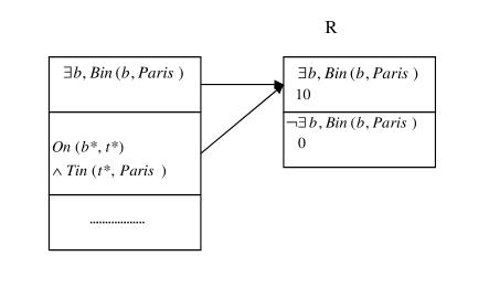
Figure 1: An example illustrating regression over the action alternative $unloadS(b^{*},t^{*})$.

After the regression, we get a parameterized $Q$-function which accounts for all possible instances of the action. We need to maximize over the action parameters of the $Q$-function to get the maximum value that could be achieved by using an instance of this action. To illustrate this step, consider the logistics example where we have two boxes $b_{1}$ and $b_{2}$, and $b_{1}$ is on truck $t_{1}$, which is in Paris (that is, $On(b_{1},t_{1})$ and $Tin(t_{1},Paris)$), while $b_{2}$ is in Boston ($Bin(b_{2},Boston)$). For the action schema $unload(b^{*},t^{*})$, we can instantiate $b^{*}$ and $t^{*}$ with $b_{1}$ and $t_{1}$ respectively, which will help us achieve the goal; or we can instantiate $b^{*}$ and $t^{*}$ with $b_{2}$ and $t_{1}$ respectively, which will have no effect. Therefore we need to perform maximization over action parameters to get the best instance of an action. Yet, we must perform this maximization generically, without knowledge of the actual state. In SDP, this is done in several steps. First, we add existential quantifiers over action parameters (which leads to non disjoint partitions). Then we sort the abstract states in $Q^{A(\vec{x})}$ by the value in decreasing order and include the negated conditions for the first $n$ abstract states in the formula for the $(n+1)^{th}$, ensuring mutual exclusion. Notice how this step leads to complex description of the resulting state partitions in SDP. This process is performed for every action separately. We call this step object maximization and denote it with $\mbox{obj-max}(Q^{A(\vec{x})})$.

Finally, to get the next value function we maximize over the $Q$-functions of different actions. These three steps provide one iteration of the VI algorithm which repeats the update until convergence.

The solutions of ReBel (?) and FOVIA (?, ?) follow the same outline but use a simpler logical language for representing RMDPs. An abstract state in ReBel is captured using an existentially quantified conjunction. FOVIA (?, ?) has a more complex representation allowing a conjunction that must hold in a state and a set of conjunctions that must be violated. An important feature in ReBel is the use of decision list (?) style representations for value functions and policies. The decision list gives us an implicit maximization operator since rules higher on the list are evaluated first. As a result the object maximization step is very simple in ReBel. Each state partition is represented implicitly by the negation of all rules above it, and explicitly by the conjunction in the rule. On the other hand, regression in ReBel requires that one enumerate all possible matches between a subset of a conjunctive goal (or state partition) and action effects, and reason about each of these separately. So this step can potentially be improved.

In the following section we introduce a new representation – First Order Decision Diagrams (FODD). FODDs allow for sharing of parts of partitions, leading to space and time saving. More importantly the value iteration algorithm based on FODDs has both simple regression and simple object maximization.

3 First Order Decision Diagrams

A decision diagram is a graphical representation for functions over propositional (Boolean) variables. The function is represented as a labeled rooted directed acyclic graph where each non-leaf node is labeled with a propositional variable and has exactly two children. The outgoing edges are marked with values true and false. Leaves are labeled with numerical values. Given an assignment of truth values to the propositional variables, we can traverse the graph where in each node we follow the outgoing edge corresponding to its truth value. This gives a mapping from any assignment to a leaf of the diagram and in turn to its value. If the leaves are marked with values in $\{0,1\}$ then we can interpret the graph as representing a Boolean function over the propositional variables. Equivalently, the graph can be seen as representing a logical expression which is satisfied if and only if the 1 leaf is reached. The case with $\{0,1\}$ leaves is known as Binary Decision Diagrams (BDDs) and the case with numerical leaves (or more general algebraic expressions) is known as Algebraic Decision Diagrams (ADDs). Decision Diagrams are particularly interesting if we impose an order over propositional variables and require that node labels respect this order on every path in the diagram; this case is known as Ordered Decision Diagrams (ODD). In this case every function has a unique canonical representation that serves as a normal form for the function. This property means that propositional theorem proving is easy for ODD representations. For example, if a formula is contradictory then this fact is evident when we represent it as a BDD, since the normal form for a contradiction is a single leaf valued $0$. This property together with efficient manipulation algorithms for ODD representations have led to successful applications, e.g., in VLSI design and verification (?, ?, ?) as well as MDPs (?, ?). In the following we generalize this representation for relational problems.

3.1 Syntax of First Order Decision Diagrams

There are various ways to generalize ADDs to capture relational structure. One could use closed or open formulas in the nodes, and in the latter case we must interpret the quantification over the variables. In the process of developing the ideas in this paper we have considered several possibilities including explicit quantifiers but these did not lead to useful solutions. We therefore focus on the following syntactic definition which does not have any explicit quantifiers.

For this representation, we assume a fixed set of predicates and constant symbols, and an enumerable set of variables. We also allow using an equality between any pair of terms (constants or variables).

Definition 1

First Order Decision Diagram

1. A First Order Decision Diagram (FODD) is a labeled rooted directed acyclic graph, where each non-leaf node has exactly two children. The outgoing edges are marked with values true and false.

2. Each non-leaf node is labeled with: an atom $P(t_{1},\ldots,t_{n})$ or an equality $t_{1}=t_{2}$ where each $t_{i}$ is a variable or a constant.

3. Leaves are labeled with numerical values.

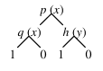
Figure 2: A simple FODD.

Figure 2 shows a FODD with binary leaves. Left going edges represent true branches. To simplify diagrams in the paper we draw multiple copies of the leaves 0 and 1 (and occasionally other values or small sub-diagrams) but they represent the same node in the FODD.

We use the following notation: for a node $n$, $n_{\downarrow t}$ denotes the true branch of $n$, and $n_{\downarrow f}$ the false branch of $n$; $n_{\downarrow a}$ is an outgoing edge from $n$, where $a$ can be true or false. For an edge $e$, $source(e)$ is the node that edge $e$ issues from, and $target(e)$ is the node that edge $e$ points to. Let $e_{1}$ and $e_{2}$ be two edges, we have $e_{1}=sibling(e_{2})$ iff $source(e_{1})=source(e_{2})$.

In the following we will slightly abuse the notation and let $n_{\downarrow a}$ mean either an edge or the sub-FODD this edge points to. We will also use $n_{\downarrow a}$ and $target(e_{1})$ interchangeably where $n=source(e_{1})$ and $a$ can be true or false depending on whether $e_{1}$ lies in the true or false branch of $n$.

3.2 Semantics of First Order Decision Diagrams

We use a FODD to represent a function that assigns values to states in a relational MDP. For example, in the logistics domain, we might want to assign values to different states in such a way that if there is a box in Paris, then the state is assigned a value of 19; if there is no box in Paris but there is a box on a truck that is in Paris and it is raining, this state is assigned a value of 6.3, and so on. The question is how to define the semantics of FODDs in order to have the intended meaning.

The semantics of first order formulas are given relative to interpretations. An interpretation has a domain of elements, a mapping of constants to domain elements and, for each predicate, a relation over the domain elements which specifies when the predicate is true. In the MDP context, a state can be captured by an interpretation. For example in the logistics domain, a state includes objects such as boxes, trucks, and cities, and relations among them, such as box 1 on truck 1 ($On(b_{1},t_{1})$), box 2 in Paris ($Bin(b_{2},Paris)$) and so on. There is more than one way to define the meaning of FODD $B$ on interpretation $I$. In the following we discuss two possibilities.

3.2.1 Semantics Based on a Single Path

A semantics for relational decision trees is given by ? (?) and it can be adapted to FODDs. The semantics define a unique path that is followed when traversing $B$ relative to $I$. All variables are existential and a node is evaluated relative to the path leading to it.

In particular, when we reach a node some of its variables have been seen before on the path and some are new. Consider a node $n$ with label $l(n)$ and the path leading to it from the root, and let $C$ be the conjunction of all labels of nodes that are exited on the true branch on the path. Then in the node $n$ we evaluate $\exists\vec{x},C\wedge l(n)$, where $\vec{x}$ includes all the variables in $C$ and $l(n)$. If this formula is satisfied in $I$ then we follow the true branch. Otherwise we follow the false branch. This process defines a unique path from the root to a leaf and its value.

For example, if we evaluate the diagram in Figure 2 on the interpretation $I_{1}$ with domain $\{1,2,3\}$ and where the only true atoms are $\{p(1),q(2),h(3)\}$ then we follow the true branch at the root since $\exists x,p(x)$ is satisfied, but we follow the false branch at $q(x)$ since $\exists x,p(x)\wedge q(x)$ is not satisfied. Since the leaf is labeled with 0 we say that $B$ does not satisfy $I$. This is an attractive approach, because it partitions the set of interpretations into mutually exclusive sets and this can be used to create abstract state partitions in the MDP context. However, for reasons we discuss later, this semantics leads to various complications for the value iteration algorithm, and it is therefore not used in the paper.

3.2.2 Semantics Based on Multiple Paths

The second alternative builds on work by ? (?) who defined semantics based on multiple paths. Following this work, we define the semantics first relative to a variable valuation $\zeta$. Given a FODD $B$ over variables $\vec{x}$ and an interpretation $I$, a valuation $\zeta$ maps each variable in $\vec{x}$ to a domain element in $I$. Once this is done, each node predicate evaluates either to true or false and we can traverse a single path to a leaf. The value of this leaf is denoted by ${\mbox{MAP}}_{B}(I,\zeta)$.

Different valuations may give different values; but recall that we use FODDs to represent a function over states, and each state must be assigned a single value. Therefore, we next define

$${\mbox{MAP}}_{B}(I)=\mbox{aggregate}_{\zeta}\{{\mbox{MAP}}_{B}(I,\zeta)\}$$

for some aggregation function. That is, we consider all possible valuations $\zeta$, and for each valuation we calculate ${\mbox{MAP}}_{B}(I,\zeta)$. We then aggregate over all these values. In the special case of ? (?) leaf labels are in $\{0,1\}$ and variables are universally quantified; this is easily captured in our formulation by using minimum as the aggregation function. In this paper we use maximum as the aggregation function. This corresponds to existential quantification in the binary case (if there is a valuation leading to value $1$, then the value assigned will be $1$) and gives useful maximization for value functions in the general case. We therefore define:

$${\mbox{MAP}}_{B}(I)=\max_{\zeta}\{{\mbox{MAP}}_{B}(I,\zeta)\}.$$

Using this definition $B$ assigns every $I$ a unique value $v={\mbox{MAP}}_{B}(I)$ so $B$ defines a function from interpretations to real values. We later refer to this function as the map of $B$.

Consider evaluating the diagram in Figure 2 on the interpretation $I_{1}$ given above where the only true atoms are $\{p(1),q(2),h(3)\}$. The valuation where $x$ is mapped to $2$ and $y$ is mapped to 3 denoted $\{x/2,y/3\}$ leads to a leaf with value 1 so the maximum is 1. When leaf labels are in {0,1}, we can interpret the diagram as a logical formula. When ${\mbox{MAP}}_{B}(I)=1$, as in our example, we say that $I$ satisfies $B$ and when ${\mbox{MAP}}_{B}(I)=0$ we say that $I$ falsifies $B$.

We define node formulas (NF) and edge formulas (EF) recursively as follows. For a node $n$ labeled $l(n)$ with incoming edges $e_{1},\ldots,e_{k}$, the node formula ${\mbox{NF}}(n)=(\vee_{i}{\mbox{EF}}(e_{i}))$. The edge formula for the true outgoing edge of $n$ is ${\mbox{EF}}(n_{\downarrow t})={\mbox{NF}}(n)\wedge l(n)$. The edge formula for the false outgoing edge of $n$ is ${\mbox{EF}}(n_{\downarrow f})={\mbox{NF}}(n)\wedge\neg l(n)$. These formulas, where all variables are existentially quantified, capture the conditions under which a node or edge are reached.

3.3 Basic Reduction of FODDs

? (?) define several operators that reduce a diagram into normal form. A total order over node labels is assumed. We describe these operators briefly and give their main properties.

(R1)

Neglect operator: if both children of a node $p$ in the FODD lead to the same node $q$ then we remove $p$ and link all parents of $p$ to $q$ directly.

(R2)

Join operator: if two nodes $p,q$ have the same label and point to the same two children then we can join $p$ and $q$ (remove $q$ and link $q$’s parents to $p$).

(R3)

Merge operator: if a node and its child have the same label then the parent can point directly to the grandchild.

(R4)

Sort operator: If a node $p$ is a parent of $q$ but the label ordering is violated ($l(p)>l(q)$) then we can reorder the nodes locally using two copies of $p$ and $q$ such that labels of the nodes do not violate the ordering.

Define a FODD to be reduced if none of the four operators can be applied. We have the following:

Theorem 1

(?) 
(1) Let $O\in\{$Neglect, Join, Merge, Sort$\}$ be an operator and $O(B)$ the result of applying $O$ to FODD $B$, then for any $B$, $I$, and $\zeta$, ${\mbox{MAP}}_{B}(I,\zeta)={\mbox{MAP}}_{O(B)}(I,\zeta)$.
(2) If $B_{1},B_{2}$ are reduced and satisfy $\forall\zeta,$ ${\mbox{MAP}}_{B_{1}}(I,\zeta)$ $={\mbox{MAP}}_{B_{2}}(I,\zeta)$ then they are identical.

Property (1) gives soundness, and property (2) shows that reducing a FODD gives a normal form. However, this only holds if the maps are identical for every $\zeta$ and this condition is stronger than normal equivalence. This normal form suffices for ? (?) who use it to provide a theorem prover for first order logic, but it is not strong enough for our purposes. Figure 3 shows two pairs of reduced FODDs (with respect to R1-R4) such that ${\mbox{MAP}}_{B_{1}}(I)={\mbox{MAP}}_{B_{2}}(I)$ but $\exists\zeta,{\mbox{MAP}}_{B_{1}}(I,\zeta)\not={\mbox{MAP}}_{B_{2}}(I,\zeta)$. In this case although the maps are the same the FODDs are not reduced to the same form. Consider first the pair in part (a) of the figure. An interpretation where $p(a)$ is false but $p(b)$ is true and a substitution $\{x/a,y/b\}$ leads to value of 0 in $B_{1}$ while $B_{2}$ always evaluates to 1. But the diagrams are equivalent. For any interpretation, if $p(c)$ is true for any object $c$ then ${\mbox{MAP}}_{B_{1}}(I)=1$ through the substitution $\{x/c\}$; if $p(c)$ is false for any object $c$ then ${\mbox{MAP}}_{B_{1}}(I)=1$ through the substitution $\{x/c,y/c\}$. Thus the map is always 1 for $B_{1}$ as well. In Section 4.2 we show that with the additional reduction operators we have developed, B1 in the first pair is reduced to $1$. Thus the diagrams in (a) have the same form after reduction. However, our reductions do not resolve the second pair given in part (b) of the figure. Notice that both functions capture a path of two edges labeled $p$ in a graph (we just change the order of two nodes and rename variables) so the diagrams evaluate to 1 if and only if the interpretation has such a path. Even though B1 and B2 are logically equivalent, they cannot be reduced to the same form using R1-R4 or our new operators. To identify a unique minimal syntactic form one may have to consider all possible renamings of variables and the sorted diagrams they produce, but this is an expensive operation. A discussion of normal form for conjunctions that uses such an operation is given by ? (?).

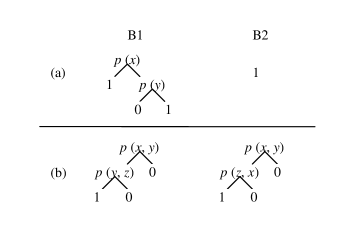
Figure 3: Examples illustrating weakness of normal form.

3.4 Combining FODDs

Given two algebraic diagrams we may need to add the corresponding functions, take the maximum or use any other binary operation, op, over the values represented by the functions. Here we adopt the solution from the propositional case (?) in the form of the procedure Apply($B_{1}$,$B_{2}$,op) where $B_{1}$ and $B_{2}$ are algebraic diagrams. Let $p$ and $q$ be the roots of $B_{1}$ and $B_{2}$ respectively. This procedure chooses a new root label (the lower among labels of $p,q$) and recursively combines the corresponding sub-diagrams, according to the relation between the two labels ($\prec$, $=$, or $\succ$). In order to make sure the result is reduced in the propositional sense one can use dynamic programming to avoid generating nodes for which either neglect or join operators ((R1) and (R2) above) would be applicable.

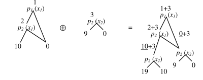
Figure 4: A simple example of adding two FODDs.

Figure 4 illustrates this process. In this example, we assume predicate ordering as $p_{1}\prec p_{2}$, and parameter ordering $x_{1}\prec x_{2}$. Non-leaf nodes are annotated with numbers and numerical leaves are underlined for identification during the execution trace. For example, the top level call adds the functions corresponding to nodes 1 and 3. Since $p_{1}(x_{1})$ is the smaller label it is picked as the label for the root of the result. Then we must add both left and right child of node 1 to node 3. These calls are performed recursively. It is easy to see that the size of the result may be the product of sizes of input diagrams. However, much pruning will occur with shared variables and further pruning is made possible by weak reductions presented later.

Since for any interpretation $I$ and any fixed valuation $\zeta$ the FODD is propositional, we have the following lemma. We later refer to this property as the correctness of Apply.

Lemma 1

Let $C=Apply(A,B,op)$, then for any $I$ and $\zeta$, ${\mbox{MAP}}_{A}(I,\zeta)\mbox{ op }{\mbox{MAP}}_{B}(I,\zeta)={\mbox{MAP}}_{C}(I,\zeta)$.

Proof: First we introduce some terminology. Let $\#nodes(X)$ refer to the set of all nodes in a FODD $X$. Let the root nodes of $A$ and $B$ be $A_{root}$ and $B_{root}$ respectively. Let the FODDs rooted at $A_{root_{\downarrow t}}$, $A_{root_{\downarrow f}}$, $B_{root_{\downarrow t}}$, $B_{root_{\downarrow f}}$, $C_{root_{\downarrow t}}$, and $C_{root_{\downarrow f}}$ be $A^{l}$, $A^{r}$, $B^{l}$, $B^{r}$, $C^{l}$ and $C^{r}$ respectively.

The proof is by induction on $n=|\#nodes(A)|+|\#nodes(B)|$. The lemma is true for $n=2$, because in this case both $A_{root}$ and $B_{root}$ have to be single leaves and an operation on them is the same as an operation on two real numbers. For the inductive step we need to consider two cases.

Case 1: $A_{root}=B_{root}$. Since the root nodes are equal, if a valuation $\zeta$ reaches $A^{l}$, then it will also reach $B^{l}$ and if $\zeta$ reaches $A^{r}$, then it will also reach $B^{r}$. Also, by the definition of Apply, in this case $C^{l}=Apply(A^{l},B^{l},op)$ and $C^{r}=Apply(A^{r},B^{r},op)$. Therefore the statement of the lemma is true if ${\mbox{MAP}}_{A^{l}}(I,\zeta)\mbox{ op }{\mbox{MAP}}_{B^{l}}(I,\zeta)={\mbox{MAP}}_{C^{l}}(I,\zeta)$ and ${\mbox{MAP}}_{A^{r}}(I,\zeta)\mbox{ op }{\mbox{MAP}}_{B^{r}}(I,\zeta)={\mbox{MAP}}_{C^{r}}(I,\zeta)$ for any $\zeta$ and $I$. Now, since $|\#nodes(A^{l})+\#nodes(B^{l})|<n$ and $|\#nodes(A^{r})+\#nodes(B^{r})|<n$, this is guaranteed by the induction hypothesis.

Case 2: $A_{root}\neq B_{root}$. Without loss of generality let us assume that $A_{root}\prec B_{root}$. By the definition of Apply, $C^{l}=Apply(A^{l},B,op)$ and $C^{r}=Apply(A^{r},B,op)$. Therefore the statement of the lemma is true if ${\mbox{MAP}}_{A^{l}}(I,\zeta)\mbox{ op }{\mbox{MAP}}_{B}(I,\zeta)={\mbox{MAP}}_{C^{l}}(I,\zeta)$ and ${\mbox{MAP}}_{A^{r}}(I,\zeta)\mbox{ op }{\mbox{MAP}}_{B}(I,\zeta)={\mbox{MAP}}_{C^{r}}(I,\zeta)$ for any $\zeta$ and $I$. Again this is guaranteed by the induction hypothesis. $\Box$

3.5 Order of Labels

The syntax of FODDs allows for two “types” of objects: constants and variables. Any argument of a predicate can be a constant or a variable. We assume a complete ordering on predicates, constants, and variables. The ordering $\prec$ between two labels is given by the following rules.

1. $P(x_{1},...,x_{n})\prec P^{\prime}(x_{1}^{\prime},...,x_{m}^{\prime})$ if $P\prec P^{\prime}$

2. $P(x_{1},...,x_{n})\prec P(x_{1}^{\prime},...,x_{n}^{\prime})$ if there exists $i$ such that $x_{j}=x_{j}^{\prime}$ for all $j<i$, and $type(x_{i})\prec type(x_{i}^{\prime})$ (where “type” can be constant or variable) or $type(x_{i})=type(x_{i}^{\prime})$ and $x_{i}\prec x_{i}^{\prime}$.

While the predicate order can be set arbitrarily it appears useful to assign the equality predicate as the first in the predicate ordering so that equalities are at the top of the diagrams. During reductions we often encounter situations where one side of the equality can be completely removed leading to substantial space savings. It may also be useful to order the argument types so that constant $\prec$ variables. This ordering may be helpful for reductions. Intuitively, a variable appearing lower in the diagram can be bound to the value of a constant that appears above it. These are only heuristic guidelines and the best ordering may well be problem dependent. We later introduce other forms of arguments: predicate parameters and action parameters. The ordering for these is discussed in Section 6.

4 Additional Reduction Operators

In our context, especially for algebraic FODDs, we may want to reduce the diagrams further. We distinguish strong reductions that preserve ${\mbox{MAP}}_{B}(I,\zeta)$ for all $\zeta$ and weak reductions that only preserve ${\mbox{MAP}}_{B}(I)$. Theorem 1 shows that R1-R4 given above are strong reductions. The details of our relational VI algorithm do not directly depend on the reductions used. Readers more interested in RMDP details can skip to Section 5 which can be read independently (except where reductions are illustrated in examples).

All the reduction operators below can incorporate existing knowledge on relationships between predicates in the domain. We denote this background knowledge by ${\cal B}$. For example in the Blocks World we may know that if there is a block on block $y$ then it is not clear: $\forall x,y,[on(x,y)\rightarrow\neg clear(y)]$.

In the following when we define conditions for reduction operators, there are two types of conditions: the reachability condition and the value condition. We name reachability conditions by starting with P (for Path Condition) and the reduction operator number. We name conditions on values by starting with V and the reduction operator number.

4.1 (R5) Strong Reduction for Implied Branches

Consider any node $n$ such that whenever $n$ is reached then the true branch is followed. In this case we can remove $n$ and connect its parents directly to the true branch. We first present the condition, followed by the lemma regarding this operator.

(P5) : ${\cal B}\models\forall\vec{x},[{\mbox{NF}}(n)\rightarrow l(n)]$ where $\vec{x}$ are the variables in ${\mbox{EF}}(n_{\downarrow t})$.

Let ${\mbox{R5}}(n)$ denote the operator that removes node $n$ and connects its parents directly to the true branch. Notice that this is a generalization of R3. It is easy to see that the following lemma is true:

Lemma 2

Let $B$ be a FODD, $n$ a node for which condition P5 holds, and $B^{\prime}$ the result of ${\mbox{R5}}(n)$. Then for any interpretation $I$ and any valuation $\zeta$ we have ${\mbox{MAP}}_{B}(I,\zeta)={\mbox{MAP}}_{B^{\prime}}(I,\zeta)$.

A similar reduction can be formulated for the false branch, i.e., if ${\cal B}\models\forall\vec{x},[{\mbox{NF}}(n)\rightarrow\neg l(n)]$ then whenever node $n$ is reached then the false branch is followed. In this case we can remove $n$ and connect its parents directly to the false branch.

Implied branches may simply be a result of equalities along a path. For example $(x=y)\wedge p(x)\rightarrow p(y)$ so we may prune $p(y)$ if $(x=y)$ and $p(x)$ are known to be true. Implied branches may also be a result of background knowledge. For example in the Blocks World if $on(x,y)$ is guaranteed to be true when we reach a node labeled $clear(y)$ then we can remove $clear(y)$ and connect its parent to $clear(y)_{\downarrow f}$.

4.2 (R7) Weak Reduction Removing Dominated Edges

Consider any two edges $e_{1}$ and $e_{2}$ in a FODD whose formulas satisfy that if we can follow $e_{2}$ using some valuation then we can also follow $e_{1}$ using a possibly different valuation. If $e_{1}$ gives better value than $e_{2}$ then intuitively $e_{2}$ never determines the value of the diagram and is therefore redundant. We formalize this as reduction operator R7.

Let $p=source(e_{1}),q=source(e_{2})$, $e_{1}=p_{\downarrow a}$, and $e_{2}=q_{\downarrow b}$, where $a$ and $b$ can be true or false. We first present all the conditions for the operator and then follow with the definition of the operator.

(P7.1) : ${\cal B}\models[\exists\vec{x},{\mbox{EF}}(e_{2})]\rightarrow[\exists\vec{y},{\mbox{EF}}(e_{1})]$ where $\vec{x}$ are the variables in ${\mbox{EF}}(e_{2})$ and $\vec{y}$ the variables in ${\mbox{EF}}(e_{1})$.

(P7.2) : ${\cal B}\models\forall\vec{u},[[\exists\vec{w},{\mbox{EF}}(e_{2})]\rightarrow[\exists\vec{v},{\mbox{EF}}(e_{1})]]$ where $\vec{u}$ are the variables that appear in both $target(e_{1})$ and $target(e_{2})$, $\vec{v}$ the variables that appear in ${\mbox{EF}}(e_{1})$ but are not in $\vec{u}$, and $\vec{w}$ the variables that appear in ${\mbox{EF}}(e_{2})$ but are not in $\vec{u}$. This condition requires that for every valuation $\zeta_{1}$ that reaches $e_{2}$ there is a valuation $\zeta_{2}$ that reaches $e_{1}$ such that $\zeta_{1}$ and $\zeta_{2}$ agree on all variables that appear in both $target(e_{1})$ and $target(e_{2})$.

(P7.3) : ${\cal B}\models\forall\vec{r},[[\exists\vec{s},{\mbox{EF}}(e_{2})]\rightarrow[\exists\vec{t},{\mbox{EF}}(e_{1})]]$ where $\vec{r}$ are the variables that appear in both $target(e_{1})$ and $target(sibling(e_{2}))$, $\vec{t}$ the variables that appear in ${\mbox{EF}}(e_{1})$ but are not in $\vec{r}$, and $\vec{s}$ the variables that appear in ${\mbox{EF}}(e_{2})$ but are not in $\vec{r}$. This condition requires that for every valuation $\zeta_{1}$ that reaches $e_{2}$ there is a valuation $\zeta_{2}$ that reaches $e_{1}$ such that $\zeta_{1}$ and $\zeta_{2}$ agree on all variables that appear in both $target(e_{1})$ and $target(sibling(e_{2}))$.

(V7.1) : $\min(target(e_{1}))\geq\max(target(e_{2}))$ where $\min(target(e_{1}))$ is the minimum leaf value in $target(e_{1})$, and $\max(target(e_{2}))$ the maximum leaf value in $target(e_{2})$. In this case regardless of the valuation we know that it is better to follow $e_{1}$ and not $e_{2}$.

(V7.2) : $\min(target(e_{1}))\geq\max(target(sibling(e_{2})))$.

(V7.3) : all leaves in $D=target(e_{1})\ominus target(e_{2})$ have non-negative values, denoted as $D\geq 0$. In this case for any fixed valuation it is better to follow $e_{1}$ instead of $e_{2}$.

(V7.4) : all leaves in $G=target(e_{1})\ominus target(sibling(e_{2}))$ have non-negative values.

We define the operators ${\mbox{R7-replace}}(b,e_{1},e_{2})$ as replacing $target(e_{2})$ with a constant $b$ that is between 0 and $\min(target(e_{1}))$ (we may write it as ${\mbox{R7-replace}}(e_{1},e_{2})$ if $b=0$), and ${\mbox{R7-drop}}(e_{1},e_{2})$ as dropping the node $q=source(e_{2})$ and connecting its parents to $target(sibling(e_{2}))$.

We need one more “safety” condition to guarantee that the reduction is correct:

(S1) : ${\mbox{NF}}(source(e_{1}))$ and the sub-FODD of $target(e_{1})$ remain the same before and after R7-replace and R7-drop. This condition says that we must not harm the value promised by $target(e_{1})$. In other words, we must guarantee that $p=source(e_{1})$ is reachable just as before and the sub-FODD of $target(e_{1})$ is not modified after replacing a branch with $0$. The condition is violated if $q$ is in the sub-FODD of $p_{\downarrow a}$, or if $p$ is in the sub-FODD of $q_{\downarrow b}$. But it holds in all other cases, that is when $p$ and $q$ are unrelated (one is not the descendant of the other), or $q$ is in the sub-FODD of $p_{\downarrow\overline{a}}$, or $p$ is in the sub-FODD of $q_{\downarrow\overline{b}}$, where $\overline{a},\overline{b}$ are the negations of $a,b$.

Lemma 3

Let $B$ be a FODD, $e_{1}$ and $e_{2}$ edges for which conditions P7.1, V7.1, and S1 hold, and $B^{\prime}$ the result of ${\mbox{R7-replace}}(b,e_{1},e_{2})$, where $0\leq b\leq\min(target(e_{1}))$, then for any interpretation $I$ we have ${\mbox{MAP}}_{B}(I)={\mbox{MAP}}_{B^{\prime}}(I)$.

Proof: Consider any valuation $\zeta_{1}$ that reaches $target(e_{2})$. Then according to P7.1, there is another valuation reaching $target(e_{1})$ and by V7.1 it gives a higher value. Therefore, ${\mbox{MAP}}_{B}(I)$ will never be determined by $target(e_{2})$ so we can replace $target(e_{2})$ with a constant between 0 and $\min(target(e_{1}))$ without changing the map. $\Box$

Lemma 4

Let $B$ be a FODD, $e_{1}$ and $e_{2}$ edges for which conditions P7.2, V7.3, and S1 hold, and $B^{\prime}$ the result of ${\mbox{R7-replace}}(b,e_{1},e_{2})$, where $0\leq b\leq\min(target(e_{1}))$, then for any interpretation $I$ we have ${\mbox{MAP}}_{B}(I)={\mbox{MAP}}_{B^{\prime}}(I)$.

Proof: Consider any valuation $\zeta_{1}$ that reaches $target(e_{2})$. By P7.2 there is another valuation $\zeta_{2}$ reaching $target(e_{1})$ and $\zeta_{1}$ and $\zeta_{2}$ agree on all variables that appear in both $target(e_{1})$ and $target(e_{2})$. Therefore, by V7.3 it achieves a higher value (otherwise, there must be a branch in $D=target(e_{1})\ominus target(e_{2})$ with a negative value). Therefore according to maximum aggregation the value of ${\mbox{MAP}}_{B}(I)$ will never be determined by $target(e_{2})$, and we can replace it with a constant as described above. $\Box$

Note that the conditions in the previous two lemmas are not comparable since P7.2 $\rightarrow$ P7.1 and V7.1 $\rightarrow$ V7.3. Intuitively when we relax the conditions on values, we need to strengthen the conditions on reachability. The subtraction operation $D=target(e_{1})\ominus target(e_{2})$ is propositional, so the test in V7.3 implicitly assumes that the common variables in the operands are the same and P7.1 does not check this. Figure 5 illustrates that the reachability condition P7.1 together with V7.3, i.e., combining the weaker portions of conditions from Lemma 3 and Lemma 4, cannot guarantee that we can replace a branch with a constant. Consider an interpretation $I$ with domain $\{1,2,3,4\}$ and relations $\{h(1,2),q(3,4),p(2)\}$. In addition assume domain knowledge ${\cal B}=[\exists x,y,h(x,y)\rightarrow\exists z,w,q(z,w)]$. So P7.1 and V7.3 hold for $e_{1}=[q(x,y)]_{\downarrow t}$ and $e_{2}=[h(z,y)_{\downarrow t}]$. We have ${\mbox{MAP}}_{B1}(I)=3$ and ${\mbox{MAP}}_{B2}(I)=0$. It is therefore not possible to replace $h(z,y)_{\downarrow t}$ with $0$.

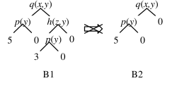
Figure 5: An example illustrating the subtraction condition in R7.

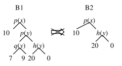
Figure 6: An example illustrating the condition for removing a node in R7.

Sometimes we can drop the node $q$ completely with R7-drop. Intuitively, when we remove a node, we must guarantee that we do not gain extra value. The conditions for R7-replace can only guarantee that we will not lose any value. But if we remove the node $q$, a valuation that was supposed to reach $e_{2}$ may reach a better value in $e_{2}$’s sibling. This would change the map, as illustrated in Figure 6. Notice that the conditions P7.1 and V7.1 hold for $e_{1}=[p(x)]_{\downarrow t}$ and $e_{2}=[p(y)]_{\downarrow t}$ so we can replace $[p(y)]_{\downarrow t}$ with a constant. Consider an interpretation $I$ with domain $\{1,2\}$ and relations $\{q(1),p(2),h(2)\}$. We have ${\mbox{MAP}}_{B1}(I)=10$ via valuation $\{x/2\}$ and ${\mbox{MAP}}_{B2}(I)=20$ via valuation $\{x/1,y/2\}$. Thus removing $p(y)$ is not correct.

Therefore we need the additional condition to guarantee that we will not gain extra value with node dropping. This condition can be stated as: for any valuation $\zeta_{1}$ that reaches $e_{2}$ and thus will be redirected to reach a value $v_{1}$ in $sibling(e_{2})$ when $q$ is removed, there is a valuation $\zeta_{2}$ that reaches a leaf with value $v_{2}\geq v_{1}$. However, this condition is too complex to test in practice. In the following we identify two stronger conditions.

Lemma 5

Let $B$ be a FODD, $e_{1}$ and $e_{2}$ edges for which condition V7.2 hold in addition to the conditions for replacing $target(e_{2})$ with a constant, and $B^{\prime}$ the result of ${\mbox{R7-drop}}(e_{1},e_{2})$, then for any interpretation $I$ we have ${\mbox{MAP}}_{B}(I)={\mbox{MAP}}_{B^{\prime}}(I)$.

Proof: Consider any valuation reaching $target(e_{2})$. As above its true value is dominated by another valuation reaching $target(e_{1})$. When we remove $q=source(e_{2})$ the valuation will reach $target(sibling(e_{2}))$ and by V7.2 the value produced is smaller than the value from $target(e_{1})$. So again the map is preserved. $\Box$

Lemma 6

Let $B$ be a FODD, $e_{1}$ and $e_{2}$ edges for which P7.3 and V7.4 hold in addition to conditions for replacing $target(e_{2})$ with a constant, and $B^{\prime}$ the result of ${\mbox{R7-drop}}(e_{1},e_{2})$, then for any interpretation $I$ we have ${\mbox{MAP}}_{B}(I)={\mbox{MAP}}_{B^{\prime}}(I)$.

Proof: Consider any valuation $\zeta_{1}$ reaching $target(e_{2})$. As above its value is dominated by another valuation reaching $target(e_{1})$. When we remove $q=source(e_{2})$ the valuation will reach $target(sibling(e_{2}))$ and by the conditions P7.3 and V7.4, the valuation $\zeta_{2}$ will reach leaf of greater value in $target(e_{1})$(otherwise there will be a branch in G leading to a negative value). So under maximum aggregation the map is not changed. $\Box$

To summarize if P7.1 and V7.1 and S1 hold or P7.2 and V7.3 and S1 hold then we can replace $target(e_{2})$ with a constant. If we can replace and V7.2 or both P7.3 and V7.4 hold then we can drop $q=source(e_{2})$ completely.

In the following we provide a more detailed analysis of applicability and variants of R7.

4.2.1 R6: A Special Case of R7

We have a special case of R7 when $p=q$, i.e., $e_{1}$ and $e_{2}$ are siblings. In this context R7 can be considered to focus on a single node $n$ instead of two edges. Assuming that $e_{1}=n_{\downarrow t}$ and $e_{2}=n_{\downarrow f}$, we can rewrite the conditions in R7 as follows.

(P7.1) : ${\cal B}\models[\exists\vec{x},{\mbox{NF}}(n)]\rightarrow[\exists\vec{x},\vec{y},{\mbox{EF}}(n_{\downarrow t})]$. This condition requires that if $n$ is reachable then $n_{\downarrow t}$ is reachable.

(P7.2) : ${\cal B}\models\forall\vec{r},[\exists\vec{v},{\mbox{NF}}(n)]\rightarrow[\exists\vec{v},\vec{w},{\mbox{EF}}(n_{\downarrow t})]$ where $\vec{r}$ are the variables that appear in both $n_{\downarrow t}$ and $n_{\downarrow f}$, $\vec{v}$ the variables that appear in ${\mbox{NF}}(n)$ but not in $\vec{r}$, and $\vec{w}$ the variables in $l(n)$ and not in $\vec{r}$ or $\vec{v}$.

(P7.3) : ${\cal B}\models\forall\vec{u},[\exists\vec{v},{\mbox{NF}}(n)]\rightarrow[\exists\vec{v},\vec{w},{\mbox{EF}}(n_{\downarrow t})]$ where $\vec{u}$ are the variables that appear in $n_{\downarrow t}$ (since $sibling(e_{2})=e_{1}$), $\vec{v}$ the variables that appear in ${\mbox{NF}}(n)$ but not in $\vec{u}$, and $\vec{w}$ the variables in $l(n)$ and not in $\vec{u}$ or $\vec{v}$.

(V7.1) : $\min(n_{\downarrow t})\geq\max(n_{\downarrow f})$.

(V7.2) : $n_{\downarrow t}$ is a constant.

(V7.3) : all leaves in the diagram $D=n_{\downarrow t}\ominus n_{\downarrow f}$ have non-negative values.

Conditions S1 and V7.4 are always true. We have previously analyzed this special case as a separate reduction operator named R6 (?). While this is a special case, it may still be useful to check for it separately before applying the generalized case of R7, as it provides large reductions and seems to occur frequently in example domains.

An important special case of R6 occurs when $l(n)$ is an equality $t_{1}=y$ where $y$ is a variable that does not occur in the FODD above node $n$. In this case, the condition P7.1 holds since we can choose the value of $y$. We can also enforce the equality in the sub-diagram of $n_{\downarrow t}$. Therefore if V7.1 holds we can remove the node $n$ connecting its parents to $n_{\downarrow t}$ and substituting $t_{1}$ for $y$ in the diagram $n_{\downarrow t}$. (Note that we may need to make copies of nodes when doing this.) In Section 4.4 we introduce a more elaborate reduction to handle equalities by taking a maximum over the left and the right children.

4.2.2 Application Order

In some cases several instances of R7 are applicable. It turns out that the order in which we apply them is important. In the following, the first example shows that the order affects the number of steps needed to reduce the diagram. The second example shows that the order affects the final result.

Consider the FODD in Figure 7(a). R7 is applicable to edges $e_{1}=[p(x_{1},y_{1})]_{\downarrow t}$ and $e_{2}=[p(x_{2},y_{2})]_{\downarrow t}$, and $e_{1}^{\prime}=[q(x_{3})]_{\downarrow t}$ and $e_{2}^{\prime}=[q(x_{2})]_{\downarrow t}$. If we reduce in a top down manner, i.e., first apply R7 on the pair $[p(x_{1},y_{1})]_{\downarrow t}$ and $[p(x_{2},y_{2})]_{\downarrow t}$, we will get the FODD in Figure 7(b), and then we apply R7 again on $[q(x_{3})]_{\downarrow t}$ and $[q(x_{2})]_{\downarrow t}$, and we will get the FODD in Figure 7(c). However, if we apply R7 first on $[q(x_{3})]_{\downarrow t}$ and $[q(x_{2})]_{\downarrow t}$ thus getting Figure 7(d), R7 cannot be applied to $[p(x_{1},y_{1})]_{\downarrow t}$ and $[p(x_{2},y_{2})]_{\downarrow t}$ because $[p(x_{1},y_{1})]_{\downarrow t}\ominus[p(x_{2},y_{2})]_{\downarrow t}$ will have negative leaves. In this case, the diagram can still be reduced. We can reduce by comparing $[q(x_{3})]_{\downarrow t}$ and $[q(x_{2})]_{\downarrow t}$ that is in the right part of FODD. We can first remove $q(x_{2})$ and get a FODD shown in Figure 7(e), and then use the neglect operator to remove $p(x_{2},y_{2})$. As we see in this example applying one instance of R7 may render other instances not applicable or may introduce more possibilities for reductions so in general we must apply the reductions sequentially. ? (?) develops conditions under which several instances of R7 can be applied simultaneously.

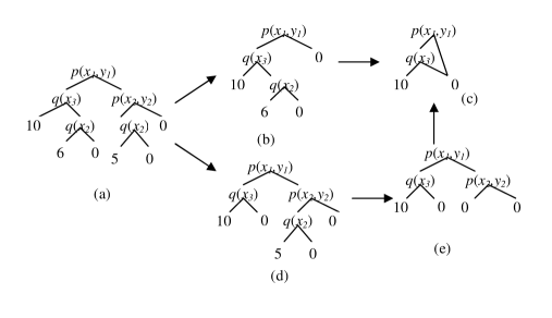
Figure 7: An example illustrating the effect of application order for R7.

One might hope that repeated application of R7 will lead to a unique reduced result but this is not true. In fact, the final result depends on the choice of operators and the order of application. Consider Figure 8(a). R7 is applicable to edges $e_{1}=[p(x)]_{\downarrow t}$ and $e_{2}=[p(y)]_{\downarrow t}$, and $e_{1}^{\prime}=[q(x)]_{\downarrow t}$ and $e_{2}^{\prime}=[q(y)]_{\downarrow t}$. If we reduce in a top down manner, i.e., first apply R7 on the pair $[p(x)]_{\downarrow t}$ and $[p(y)]_{\downarrow t}$, we will get the FODD in Figure 8(b), which cannot be reduced using existing reduction operators (including the operator R8 introduced below). However, if we apply R7 first on $[q(x)]_{\downarrow t}$ and $[q(y)]_{\downarrow t}$ we will get Figure 8(c). Then we can apply R7 again on $e_{1}=[p(x)]_{\downarrow t}$ and $e_{2}=[p(y)]_{\downarrow t}$ and get the final result Figure 8(d), which is clearly more compact than Figure 8(b). It is interesting that the first example seems to suggest applying R7 in a top down manner (since it takes fewer steps), while the second seems to suggest the opposite (since the final result is more compact). More research is needed to develop useful heuristics to guide the choice of reductions and the application order and in general develop a more complete set of reductions.

Note that we could also consider generalizing R7. In Figure 8(b), if we can reach $[q(y)]_{\downarrow t}$ then clearly we can reach $[p(x)]_{\downarrow t}$ or $[q(x)]_{\downarrow t}$. Since both $[p(x)]_{\downarrow t}$ and $[q(x)]_{\downarrow t}$ give better values, we can safely replace $[q(y)]_{\downarrow t}$ with $0$, thus obtaining the final result Figure 8(d). In theory we can generalize P7.1 as ${\cal B}\models[\exists\vec{x},{\mbox{EF}}(e_{2})]\rightarrow[\exists\vec{y_{1}},{\mbox{EF}}(e_{11})]\vee\cdots\vee[\exists\vec{y_{n}},{\mbox{EF}}(e_{1n})]$ where $\vec{x}$ are the variables in ${\mbox{EF}}(e_{2})$ and $\vec{y_{i}}$ the variables in ${\mbox{EF}}(e_{1i})$ where $1\leq i\leq n$, and generalize the corresponding value condition V7.1 as $\forall i\in[1,n],\min(target(e_{1i}))\geq\max(target(e_{2}))$. We can generalize other reachability and value conditions similarly. However the resulting conditions are too expensive to test in practice.

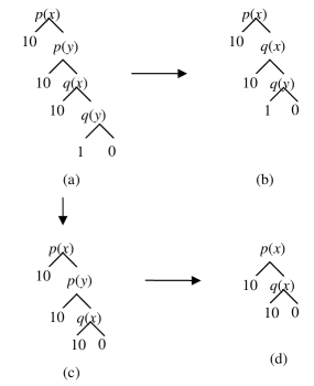
Figure 8: An example illustrating that the final result of R7 reductions is order dependent.

4.2.3 Relaxation of Reachability Conditions

The conditions P7.2 and P7.3 are sufficient, but not necessary to guarantee correct reductions. Sometimes valuations just need to agree on a smaller set of variables than the intersection of variables. To see this, consider the example as shown in Figure 9, where $A\ominus B>0$ and the intersection is $\{x,y,z\}$. However, to guarantee $A\ominus B>0$ we just need to agree on either $\{x,y\}$ or $\{x,z\}$. Intuitively we have to agree on the variable $x$ to avoid the situation when two paths $p(x,y)\wedge\neg q(x)$ and $p(x,y)\wedge q(x)\wedge h(z)$ can co-exist. In order to prevent the co-existence of two paths $\neg p(x,y)\wedge\neg h(z)$ and $p(x,y)\wedge q(x)\wedge h(z)$, either $y$ or $z$ has to be the same as well. Now if we change this example a little bit and replace each $h(z)$ with $h(z,v)$, then we have two minimal sets of variables of different size, one is $\{x,y\}$, and the other is $\{x,z,v\}$. As a result we cannot identify a minimum set of variables for the subtraction and must either choose the intersection or heuristically identify a minimal set, for example, using a greedy procedure.

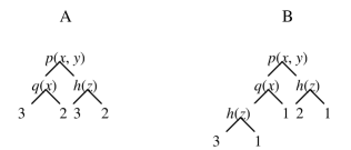
Figure 9: An example illustrating that the minimal set of variables for subtraction is not unique.

4.3 (R8) Weak Reduction by Unification

Consider a FODD $B$. Let $\vec{v}$ denote its variables, and let $\vec{x}$ and $\vec{y}$ be disjoint subsets of $\vec{v}$, which are of the same cardinality. We define the operator ${\mbox{R8}}(B,\vec{x},\vec{y})$ as replacing variables in $\vec{x}$ by the corresponding variables in $\vec{y}$. We denote the resulting FODD by $B\{\vec{x}/\vec{y}\}$ so the result has variables in $\vec{v}$ \$\vec{x}$. We have the following condition for the correctness of R8:

(V8) : all leaves in $B\{\vec{x}/\vec{y}\}\ominus B$ are non negative.

Lemma 7

Let $B$ be a FODD, $B^{\prime}$ the result of ${\mbox{R8}}(B,\vec{x},\vec{y})$ for which V8 holds, then for any interpretation $I$ we have ${\mbox{MAP}}_{B}(I)={\mbox{MAP}}_{B^{\prime}}(I)$.

Proof: Consider any valuation $\zeta_{1}$ to $\vec{v}$ in $B$. By V8, $B\{\vec{x}/\vec{y}\}$ gives a better value on the same valuation. Therefore we do not lose any value by this operator. We also do not gain any extra value. Consider any valuation $\zeta_{2}$ to variables in $B^{\prime}$ reaching a leaf node with value $v$, we can construct a valuation $\zeta_{3}$ to $\vec{v}$ in $B$ with all variables in $\vec{x}$ taking the corresponding value in $\vec{y}$, and it will reach a leaf node in $B$ with the same value. Therefore the map will not be changed by unification. $\Box$

Figure 10 illustrates that in some cases R8 is applicable where R7 is not. We can apply R8 with $\{x_{1}/x_{2}\}$ to get a FODD as shown in Figure 10(b). Since $(b)\ominus(a)\geq 0$, $(b)$ becomes the result after reduction. Note that if we unify in the other way, i.e.,$\{x_{2}/x_{1}\}$, we will get Figure 10(c), it is isomorphic to Figure 10(b), but we cannot reduce the original FODD to this result, because $(c)\ominus(a)\not\geq 0$. This phenomenon happens since the subtraction operation (implemented by Apply) used in the reductions is propositional and therefore sensitive to variable names.

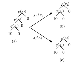
Figure 10: An example illustrating R8.

4.4 (R9) Equality Reduction

Consider a FODD $B$ with an equality node $n$ labeled $t=x$. Sometimes we can drop $n$ and connect its parents to a sub-FODD that is the result of taking the maximum of the left and the right children of $n$. For this reduction to be applicable $B$ has to satisfy the following condition.

(E9.1) : For an equality node $n$ labeled $t=x$ at least one of $t$ and $x$ is a variable and it appears neither in $n_{\downarrow f}$ nor in the node formula for $n$. To simplify the description of the reduction procedure below, we assume that $x$ is that variable.

Additionally we make the following assumption about the domain.

(D9.1) : The domain contains more than one object.

The above assumption guarantees that valuations reaching the right child of equality nodes exist. This fact is needed in proving correctness of the Equality reduction operator. First we describe the reduction procedure for ${\mbox{R9}}(n)$. Let $B_{n}$ denote the FODD rooted at node $n$ in FODD $B$. We extract a copy of $B_{n_{\downarrow t}}$ (and name it $B_{n_{\downarrow t}}\mbox{-copy}$), and a copy of $B_{n_{\downarrow f}}$ ($B_{n_{\downarrow f}}\mbox{-copy}$) from $B$. In $B_{n_{\downarrow t}}\mbox{-copy}$, we rename the variable $x$ to $t$ to produce diagram $B^{\prime}_{n_{\downarrow t}}\mbox{-copy}$. Let $B_{n}^{\prime}=Apply(B^{\prime}_{n_{\downarrow t}}\mbox{-copy},B_{n_{\downarrow f}}\mbox{-copy},max)$. Finally we drop the node $n$ in $B$ and connect its parents to the root of $B_{n}^{\prime}$ to obtain the final result $B^{\prime}$. An example is shown in Figure 11.

Informally, we are extracting the parts of the FODD rooted at node $n$, one where $x=t$ (and renaming $x$ to $t$ in that part) and one where $x\neq t$. The condition E9.1 and the assumption D9.1 guarantee that regardless of the value of $t$, we have valuations reaching both parts. Since by the definition of MAP, we maximize over the valuations, in this case we can maximize over the diagram structure itself. We do this by calculating the function which is the maximum of the two functions corresponding to the two children of $n$ (using $Apply$) and replacing the old sub-diagram rooted at node $n$ by the new combined diagram. Theorem 9 proves that this does not affect the map of $B$.

One concern for implementation is that we simply replace the old sub-diagram by the new sub-diagram, which may result in a diagram where strong reductions are applicable. While this is not a problem semantically, we can avoid the need for strong reductions by using $Apply$ that implicitly performs strong reductions R1(neglect) and R2(join) as follows.

Let $B_{a}$ denote the FODD resulting from replacing node $n$ in $B$ with $0$, and $B_{b}$ the FODD resulting from replacing node $n$ with $1$ and all leaves other than node $n$ by $0$, we have the final result $B^{\prime}=B_{a}\oplus B_{b}^{\prime}$ where $B_{b}^{\prime}=B_{b}\otimes B_{n}^{\prime}$. By correctness of $Apply$ the two forms of calculating $B^{\prime}$ give the same map.

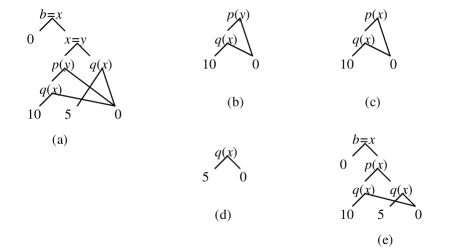
Figure 11: An example of the equality reduction. (a) The FODD before reduction. The node $x=y$ satisfies condition E9.1 for variable $y$. (b) $B_{n_{\downarrow t}}\mbox{-copy}$ ($n_{\downarrow t}$ extracted). (c) $B_{n_{\downarrow t}}\mbox{-copy}$ renamed to produce $B^{\prime}_{n_{\downarrow t}}\mbox{-copy}$. (d) $B_{n_{\downarrow f}}\mbox{-copy}$. (e) Final result with node $n$ replaced by $apply(B^{\prime}_{n_{\downarrow t}}\mbox{-copy},B_{n_{\downarrow f}}\mbox{-copy},max)$

In the following we prove that for any node $n$ where equality condition E9.1 holds in $B$ we can perform the equality reduction R9 without changing the map for any interpretation satisfying D9.1. We start with properties of FODDs defined above, e.g., $B_{a}$, $B_{b}$, and $B_{b}^{\prime}$. Let $\Gamma_{n}$ denote the set of all valuations reaching node $n$ and let $\Gamma_{m}$ denote the set of all valuations not reaching node $n$ in B. From the basic definition of MAP we have the following:

Claim 1

For any interpretation $I$,
(a) $\forall$ $\zeta\in\Gamma_{m}$, ${\mbox{MAP}}_{B_{a}}(I,\zeta)={\mbox{MAP}}_{B}(I,\zeta)$.
(b) $\forall$ $\zeta\in\Gamma_{n}$, ${\mbox{MAP}}_{B_{a}}(I,\zeta)=0$.
(c) $\forall$ $\zeta\in\Gamma_{m}$, ${\mbox{MAP}}_{B_{b}}(I,\zeta)=0$.
(d) $\forall$ $\zeta\in\Gamma_{n}$, ${\mbox{MAP}}_{B_{b}}(I,\zeta)=1$.

From Claim 1 and the definition of MAP, we have,

Claim 2

For any interpretation $I$,
(a) $\forall$ $\zeta\in\Gamma_{m}$, ${\mbox{MAP}}_{B_{b}^{\prime}}(I,\zeta)=0$.
(b) $\forall$ $\zeta\in\Gamma_{n}$, ${\mbox{MAP}}_{B_{b}^{\prime}}(I,\zeta)={\mbox{MAP}}_{B^{\prime}_{n}}(I,\zeta)$.

From Claim 1, Claim 2, and the definition of MAP we have,

Claim 3

For any interpretation $I$,
(a) $\forall$ $\zeta\in\Gamma_{m}$, ${\mbox{MAP}}_{B^{\prime}}(I,\zeta)={\mbox{MAP}}_{B}(I,\zeta)$.
(b) $\forall$ $\zeta\in\Gamma_{n}$, ${\mbox{MAP}}_{B^{\prime}}(I,\zeta)={\mbox{MAP}}_{B^{\prime}_{n}}(I,\zeta)$.

Next we prove the main property of this reduction stating that for all valuations reaching node $n$ in $B$, the old sub-FODD rooted at $n$ and the new (combined) sub-FODD produce the same map.

Lemma 8

Let $\Gamma_{n}$ be the set of valuations reaching node $n$ in FODD $B$. For any interpretation $I$ satisfying D9.1, $\max_{\zeta\in\Gamma_{n}}{\mbox{MAP}}_{B_{n}}(I,\zeta)=\max_{\zeta\in\Gamma_{n}}{\mbox{MAP}}_{B^{\prime}_{n}}(I,\zeta)$.

Proof: By condition E9.1, the variable $x$ does not appear in $NF(n)$ and hence its value in $\zeta\in\Gamma_{n}$ is not constrained. We can therefore partition the valuations in $\Gamma_{n}$ into disjoint sets, $\Gamma_{n}=\{\Gamma_{\Delta}\mid\Delta\mbox{ is a valuation to variables other than }x\}$, where in $\Gamma_{\Delta}$ variables other than $x$ are fixed to their value in $\Delta$ and $x$ can take any value in the domain of $I$. Assumption D9.1 guarantees that every $\Gamma_{\Delta}$ contains at least one valuation reaching $B_{n_{\downarrow t}}$ and at least one valuation reaching $B_{n_{\downarrow f}}$ in $B$. Note that if a valuation $\zeta$ reaches $B_{n_{\downarrow t}}$ then $t=x$ is satisfied by $\zeta$ thus ${\mbox{MAP}}_{B_{n_{\downarrow t}}}(I,\zeta)={\mbox{MAP}}_{B^{\prime}_{n_{\downarrow t}}\mbox{-copy}}(I,\zeta)$. Since $x$ does not appear in $B_{n_{\downarrow f}}$ we also have that ${\mbox{MAP}}_{B^{\prime}_{n_{\downarrow f}}\mbox{-copy}}(I,\zeta)$ is constant for all $\zeta\in\Gamma_{\Delta}$. Therefore by the correctness of $Apply$ we have $\max_{\zeta\in\Gamma_{\Delta}}{\mbox{MAP}}_{B_{n}}(I,\zeta)=\max_{\zeta\in\Gamma_{\Delta}}{\mbox{MAP}}_{B_{n}^{\prime}}(I,\zeta)$.

Finally, by the definition of MAP, $\max_{\zeta\in\Gamma_{n}}{\mbox{MAP}}_{B_{n}}(I,\zeta)=\max_{\Delta}\max_{\zeta\in\Gamma_{\Delta}}{\mbox{MAP}}_{B_{n}}(I,\zeta)$ $=\max_{\Delta}\max_{\zeta\in\Gamma_{\Delta}}{\mbox{MAP}}_{B_{n}^{\prime}}(I,\zeta)=\max_{\zeta\in\Gamma_{n}}{\mbox{MAP}}_{B_{n}}(I,\zeta)$. $\Box$

Lemma 9

Let $B$ be a FODD, $n$ a node for which condition E9.1 holds, and $B^{\prime}$ be the result of ${\mbox{R9}}(n)$, then for any interpretation $I$ satisfying D9.1, ${\mbox{MAP}}_{B}(I)={\mbox{MAP}}_{B^{\prime}}(I)$.

Proof: Let $X=\max_{\zeta\in\Gamma_{m}}{\mbox{MAP}}_{B^{\prime}}(I,\zeta)$ and $Y=\max_{\zeta\in\Gamma_{n}}{\mbox{MAP}}_{B^{\prime}}(I,\zeta)$. By the definition of MAP, ${\mbox{MAP}}_{B^{\prime}}(I)=max(X,Y)$. However, by Claim 3, $X=\max_{\zeta\in\Gamma_{m}}{\mbox{MAP}}_{B}(I,\zeta)$ and by Claim 3 and Lemma 8, $Y=\max_{\zeta\in\Gamma_{n}}{\mbox{MAP}}_{B^{\prime}_{n}}(I,\zeta)=\max_{\zeta\in\Gamma_{n}}{\mbox{MAP}}_{B_{n}}(I,\zeta)$. Thus $max(X,Y)={\mbox{MAP}}_{B}(I)={\mbox{MAP}}_{B^{\prime}}(I)$. $\Box$

While Lemma 9 guarantees correctness, when applying it in practice it may be important to avoid violations of the sorting order (which would require expensive re-sorting of the diagram). If both $x$ and $t$ are variables we can sometimes replace both with a new variable name so the resulting diagram is sorted. However this is not always possible. When such a violation is unavoidable, there is a tradeoff between performing the reduction and sorting the diagram and ignoring the potential reduction.

To summarize, this section introduced several new reductions that can compress diagrams significantly. The first (R5) is a generic strong reduction that removes implied branches in a diagram. The other three (R7, R8, R9) are weak reductions that do not alter the overall map of the diagram but do alter the map for specific valuations. The three reductions are complementary since they capture different opportunities for space saving.

5 Decision Diagrams for MDPs

In this section we show how FODDs can be used to capture a RMDP. We therefore use FODDs to represent the domain dynamics of deterministic action alternatives, the probabilistic choice of action alternatives, the reward function, and value functions.

5.1 Example Domain

We first give a concrete formulation of the logistics problem discussed in the introduction. This example follows exactly the details given by ? (?), and is used to illustrate our constructions for MDPs. The domain includes boxes, trucks and cities, and predicates are $Bin(Box,City)$, $Tin(Truck,City)$, and $On(Box,Truck)$. Following ? (?), we assume that $On(b,t)$ and $Bin(b,c)$ are mutually exclusive, so a box on a truck is not in a city and vice versa. That is, our background knowledge includes statements $\forall b,c,t,On(b,t)\rightarrow\neg Bin(b,c)$ and $\forall b,c,t,Bin(b,c)\rightarrow\neg On(b,t)$. The reward function, capturing a planning goal, awards a reward of 10 if the formula $\exists b,Bin(b,Paris)$ is true, that is if there is any box in Paris. Thus the reward is allowed to include constants but need not be completely ground.

The domain includes 3 actions $load,unload$, and $drive$. Actions have no effect if their preconditions are not met. Actions can also fail with some probability. When attempting $load$, a successful version $loadS$ is executed with probability 0.99, and an unsuccessful version $loadF$ (effectively a no-operation) with probability 0.01. The drive action is executed deterministically. When attempting $unload$, the probabilities depend on whether it is raining or not. If it is not raining then a successful version $unloadS$ is executed with probability 0.9, and $unloadF$ with probability 0.1. If it is raining $unloadS$ is executed with probability 0.7, and $unloadF$ with probability 0.3.

5.2 The Domain Dynamics

We follow ? (?) and specify stochastic actions as a randomized choice among deterministic alternatives. The domain dynamics are defined by truth value diagrams (TVDs). For every action schema $A(\vec{a})$ and each predicate schema $p(\vec{x})$ the TVD $T(A(\vec{a}),p(\vec{x}))$ is a FODD with $\{0,1\}$ leaves. The TVD gives the truth value of $p(\vec{x})$ in the next state when $A(\vec{a})$ has been performed in the current state. We call $\vec{a}$ action parameters, and $\vec{x}$ predicate parameters. No other variables are allowed in the TVD; the reasoning behind this restriction is explained in Section 6.2. The restriction can be sometimes sidestepped by introducing more action parameters instead of the variables.

The truth value of a TVD is valid when we fix a valuation of the parameters. The TVD simultaneously captures the truth values of all instances of $p(\vec{x})$ in the next state. Notice that TVDs for different predicates are separate. This can be safely done even if an action has coordinated effects (not conditionally independent) since the action alternatives are deterministic.

Since we allow both action parameters and predicate parameters, the effects of an action are not restricted to predicates over action arguments so TVD are more expressive than simple STRIPS based schemas. For example, TVDs can easily express universal effects of an action. To see this note that if $p(\vec{x})$ is true for all $\vec{x}$ after action $A(\vec{a})$ then the TVD $T(A(\vec{a}),p(\vec{x}))$ can be captured by a leaf valued 1. Other universal conditional effects can be captured similarly. On the other hand, since we do not have explicit universal quantifiers, TVDs cannot capture universal preconditions.

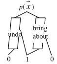
Figure 12: A template for the TVD

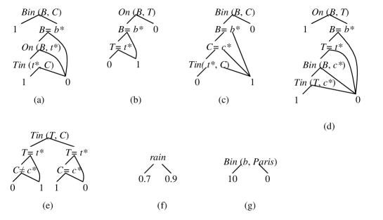
Figure 13: FODDs for logistics domain: TVDs, action choice, and reward function. (a)(b) The TVDs for $Bin(B,C)$ and $On(B,T)$ under action choice $unloadS(b^{*},t^{*})$. (c)(d) The TVDs for $Bin(B,C)$ and $On(B,T)$ under action choice $loadS(b^{*},t^{*},c^{*})$. Note that $c^{*}$ must be an action parameter so that (d) is a valid TVD. (e) The TVD for $Tin(T,C)$ under action choice $driveS(t^{*},c^{*})$. (f) The probability FODD for the action choice $unloadS(b^{*},t^{*})$. (g) The reward function.

For any domain, a TVD for predicate $p(\vec{x})$ can be defined generically as in Figure 12. The idea is that the predicate is true if it was true before and is not “undone” by the action or was false before and is “brought about” by the action. TVDs for the logistics domain in our running example are given in Figure 13. All the TVDs omitted in the figure are trivial in the sense that the predicate is not affected by the action. In order to simplify the presentation we give the TVDs in their generic form and did not sort the diagrams using the order proposed in Section 3.5; the TVDs are consistent with the ordering $Bin\prec$ “=” $\prec On\prec Tin\prec rain$. Notice that the TVDs capture the implicit assumption usually taken in such planning-based domains that if the preconditions of the action are not satisfied then the action has no effect.

Notice how we utilize the multiple path semantics with maximum aggregation. A predicate is true if it is true according to one of the paths specified so we get a disjunction over the conditions for free. If we use the single path semantics of ? (?) the corresponding notion of TVD is significantly more complicated since a single path must capture all possibilities for a predicate to become true. To capture that, we must test sequentially for different conditions and then take a union of the substitutions from different tests and in turn this requires additional annotation on FODDs with appropriate semantics. Similarly an OR operation would require union of substitutions, thus complicating the representation. We explain these issues in more detail in Section 6.3 after we introduce the first order value iteration algorithm.

5.3 Probabilistic Action Choice

One can consider modeling arbitrary conditions described by formulas over the state to control nature’s probabilistic choice of action. Here the multiple path semantics makes it hard to specify mutually exclusive conditions using existentially quantified variables and in this way specify a distribution. We therefore restrict the conditions to be either propositional or depend directly on the action parameters. Under this condition any interpretation follows exactly one path (since there are no variables and thus only the empty valuation) thus the aggregation function does not interact with the probabilities assigned. A diagram showing action choice for $unloadS$ in our logistics example is given in Figure 13. In this example, the condition is propositional. The condition can also depend on action parameters, for example, if we assume that the result is also affected by whether the box is big or not, we can have a diagram as in Figure 14 specifying the action choice probability.

Figure 14: An example showing that the choice probability can depend on action parameters.

Note that a probability usually depends on the current state. It can depend on arbitrary properties of the state (with the restriction stated as above), e.g., $rain$ and $big(b^{*})$, as shown in Figure 14. We allow arbitrary conditions that depend on predicates with arguments restricted to action parameters so the dependence can be complex. However, we do not allow any free variables in the probability choice diagram. For example, we cannot model a probabilistic choice of $unloadS(b^{*},t^{*})$ that depends on other boxes on the truck $t^{*}$, e.g., $\exists b,On(b,t^{*})\wedge b\neq b^{*}:0.2$; otherwise, $0.7$. While we can write a FODD to capture this condition, the semantics of FODD means that a path to $0.7$ will be selected by max aggregation so the distribution cannot be modeled in this way. While this is clearly a restriction, the conditions based on action arguments still give a substantial modeling power.

5.4 Reward and Value Functions

Reward and value functions can be represented directly using algebraic FODDs. The reward function for our logistics domain example is given in Figure 13.

6 Value Iteration with FODDs

Following ? (?) we define the first order value iteration algorithm as follows: given the reward function $R$ and the action model as input, we set $V_{0}=R,n=0$ and repeat the procedure Rel-greedy until termination:

Procedure 1

Rel-greedy
1. For each action type $A(\vec{x})$, compute:

$$Q_{V_{n}}^{A(\vec{x})}=R\oplus[\gamma\otimes\oplus_{j}(prob(A_{j}(\vec{x}))\otimes Regr(V_{n},A_{j}(\vec{x})))]$$ (3)

2. $Q_{V_{n}}^{A}=\mbox{obj-max}(Q_{V_{n}}^{A(\vec{x})})$.
3. $V_{n+1}=\max_{A}Q_{V_{n}}^{A}$.

The notation and steps of this procedure were discussed in Section 2 except that now $\otimes$ and $\oplus$ work on FODDs instead of case statements. Note that since the reward function does not depend on actions, we can move the object maximization step forward before adding the reward function. I.e., we first have

$$T_{V_{n}}^{A(\vec{x})}=\oplus_{j}(prob(A_{j}(\vec{x}))\otimes Regr(V_{n},A_{j}(\vec{x}))),$$

followed by

$$Q_{V_{n}}^{A}=R\oplus\gamma\otimes\mbox{obj-max}(T_{V_{n}}^{A(\vec{x})}).$$

Later we will see that the object maximization step makes more reductions possible; therefore by moving this step forward we get some savings in computation. We compute the updated value function in this way in the comprehensive example of value iteration given later in Section 6.8.

Value iteration terminates when $\|V_{i+1}-V_{i}\|\leq\frac{\varepsilon(1-\gamma)}{2\gamma}$ (?). In our case we need to test that the values achieved by the two diagrams is within $\frac{\varepsilon(1-\gamma)}{2\gamma}$.

Some formulations of goal based planning problems use an absorbing state with zero additional reward once the goal is reached. We can handle this formulation when there is only one non-zero leaf in $R$. In this case, we can replace Equation 3 with

$$Q_{V_{n}}^{A(\vec{x})}=max(R,\gamma\otimes\oplus_{j}(prob(A_{j}(\vec{x}))\otimes Regr(V_{n},A_{j}(\vec{x}))).$$

To see why this is correct, note that due to discounting the max value is always $\leq R$. If $R$ is satisfied in a state we do not care about the action (max would be $R$) and if $R$ is $0$ in a state we get the value of the discounted future reward.

Note that we can only do this in goal based domains, i.e., there is only one non-zero leaf. This does not mean that we cannot have disjunctive goals, but it means that we must value each goal condition equally.

6.1 Regressing Deterministic Action Alternatives

We first describe the calculation of $Regr(V_{n},A_{j}(\vec{x}))$ using a simple idea we call block replacement. We then proceed to discuss how to obtain the result efficiently.

Consider $V_{n}$ and the nodes in its FODD. For each such node take a copy of the corresponding TVD, where predicate parameters are renamed so that they correspond to the node’s arguments and action parameters are unmodified. $\mbox{BR-regress}(V_{n},A(\vec{x}))$ is the FODD resulting from replacing each node in $V_{n}$ with the corresponding TVD, with outgoing edges connected to the 0, 1 leaves of the TVD.

Recall that a RMDP represents a family of concrete MDPs each generated by choosing a concrete instantiation of the state space (typically represented by the number of objects and their types). The formal properties of our algorithms hold for any concrete instantiation.

Fix any concrete instantiation of the state space. Let $s$ denote a state resulting from executing an action $A(\vec{x})$ in state $\hat{s}$. Notice that $V_{n}$ and $\mbox{BR-regress}(V_{n},A(\vec{x}))$ have exactly the same variables. We have the following lemma:

Lemma 10

Let $\zeta$ be any valuation to the variables of $V_{n}$ (and thus also the variables of $\mbox{BR-regress}(V_{n},A(\vec{x}))$). Then ${\mbox{MAP}}_{V_{n}}(s,\zeta)={\mbox{MAP}}_{BR-regress(V_{n},A(\vec{x}))}(\hat{s},\zeta)$.

Proof: Consider the paths $P,\hat{P}$ followed under the valuation $\zeta$ in the two diagrams. By the definition of TVDs, the sub-paths of $\hat{P}$ applied to $\hat{s}$ guarantee that the corresponding nodes in $P$ take the same truth values in $s$. So $P,\hat{P}$ reach the same leaf and the same value is obtained. $\Box$

A naive implementation of block replacement may not be efficient. If we use block replacement for regression then the resulting FODD is not necessarily reduced and moreover, since the different blocks are sorted to start with the result is not even sorted. Reducing and sorting the results may be an expensive operation. Instead we calculate the result as follows. For any FODD $V_{n}$ we traverse $\mbox{BR-regress}(V_{n},A(\vec{x}))$ using postorder traversal in terms of blocks and combine the blocks. At any step we have to combine up to 3 FODDs such that the parent block has not yet been processed (so it is a TVD with binary leaves) and the two children have been processed (so they are general FODDs). If we call the parent $B_{n}$, the true branch child $B_{t}$ and the false branch child $B_{f}$ then we can represent their combination as $[B_{n}\otimes B_{t}]\oplus[(1\ominus B_{n})\otimes B_{f}]$.

Lemma 11

Let $B$ be a FODD where $B_{t}$ and $B_{f}$ are FODDs, and $B_{n}$ is a FODD with $\{0,1\}$ leaves. Let $\hat{B}$ be the result of using Apply to calculate the diagram $[B_{n}\otimes B_{t}]\oplus[(1\ominus B_{n})\otimes B_{f}]$. Then for any interpretation $I$ and valuation $\zeta$ we have ${\mbox{MAP}}_{B}(I,\zeta)={\mbox{MAP}}_{\hat{B}}(I,\zeta)$.

Proof: This is true since by fixing the valuation we effectively ground the FODD and all paths are mutually exclusive. In other words the FODD becomes propositional and clearly the combination using propositional Apply is correct. $\Box$

A high-level description of the algorithm to calculate $\mbox{BR-regress}(V_{n},A(\vec{x}))$ by block combination is as follows:

Procedure 2

Block Combination for $\mbox{BR-regress}(V_{n},A(\vec{x}))$

1. Perform a topological sort on $V_{n}$ nodes (see for example ?).

2. In reverse order, for each non-leaf node $n$ (its children $B_{t}$ and $B_{f}$ have already been processed), let $B_{n}$ be a copy of the corresponding TVD, calculate $[B_{n}\otimes B_{t}]\oplus[(1\ominus B_{n})\otimes B_{f}]$.

3. Return the FODD corresponding to the root.

Notice that different blocks share variables so we cannot perform weak reductions during this process. However, we can perform strong reductions in intermediate steps since they do not change the map for any valuation. After the process is completed we can perform any combination of weak and strong reductions since this does not change the map of the regressed value function.

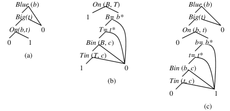
Figure 15: An example illustrating why variables are not allowed in TVDs.

We can now explain why we cannot have variables in TVDs through an example illustrated in Figure 15. Suppose we have a value function as defined in Figure 15(a), saying that if there is a blue block and a big truck such that the block is not on the truck then value $1$ is assigned. Figure 15(b) gives the TVD for $On(B,T)$ under action $loadS$, in which $c$ is a variable instead of an action parameter. Figure 15(c) gives the result after block replacement. Consider an interpretation $\hat{s}$ with domain $\{b_{1},t_{1},c_{1},c_{2}\}$ and relations $\{Blue(b_{1}),Big(t_{1}),Bin(b_{1},c_{1}),Tin(t_{1},c_{1})\}$. After the action $loadS(b_{1},t_{1})$ we will reach the state $s=\{Blue(b_{1}),Big(t_{1}),On(b_{1},t_{1}),Tin(t_{1},c_{1})\}$, which gives us a value of $0$. But Figure 15(c) with $b^{*}=b_{1},t^{*}=t_{1}$ evaluated in $\hat{s}$ gives value of 1 by valuation $\{b/b_{1},c/c_{2},t/t_{1}\}$. Here the choice $c/c_{2}$ makes sure the precondition is violated. By making $c$ an action parameter, applying the action must explicitly choose a valuation and this leads to a correct value function. Object maximization turns action parameters into variables and allows us to choose the argument so as to maximize the value.

6.2 Regressing Probabilistic Actions

To regress a probabilistic action we must regress all its deterministic alternatives and combine each with its choice probability as in Equation 3. As discussed in Section 2, due to the restriction in the RMDP model that explicitly specifies a finite number of deterministic action alternatives, we can replace the potentially infinite sum of Equation 1 with the finite sum of Equation 3. If this is done correctly for every state then the result of Equation 3 is correct. In the following we specify how this can be done with FODDs.

Recall that $prob(A_{j}(\vec{x}))$ is restricted to include only action parameters and cannot include variables. We can therefore calculate $prob(A_{j}(\vec{x}))\otimes Regr(V_{n},A_{j}(\vec{x}))$ in step (1) directly using Apply. However, the different regression results are independent functions so that in the sum $\oplus_{j}(prob(A_{j}(\vec{x}))\otimes Regr(V_{n},A_{j}(\vec{x})))$ we must standardize apart the different regression results before adding the functions (note that action parameters are still considered constants at this stage). The same holds for the addition of the reward function. The need to standardize apart complicates the diagrams and often introduces structure that can be reduced. When performing these operations we first use the propositional Apply procedure and then follow with weak and strong reductions.

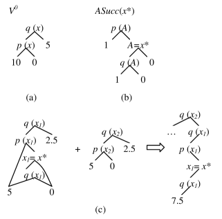
Figure 16: An example illustrating the need to standardize apart.

Figure 16 illustrates why we need to standardize apart different action outcomes. Action $A$ can succeed (denoted as $ASucc$) or fail (denoted as $AFail$, effectively a no-operation), and each is chosen with probability 0.5. Part (a) gives the value function $V^{0}$. Part (b) gives the TVD for $P(A)$ under the action choice $ASucc(x^{*})$. All other TVDs are trivial. Part (c) shows part of the result of adding the two outcomes for $A$ after standardizing apart (to simplify the presentation the diagrams are not sorted). Consider an interpretation with domain $\{1,2\}$ and relations $\{q(1),p(2)\}$. As can be seen from (c), by choosing $x^{*}=1$, i.e. action $A(1)$, the valuation $x_{1}=1,x_{2}=2$ gives a value of $7.5$ after the action (without considering the discount factor). Obviously if we do not standardize apart (i.e $x_{1}=x_{2}$), there is no leaf with value $7.5$ and we get a wrong value. Intuitively the contribution of $ASucc$ to the value comes from the “bring about” portion of the diagram and $AFail$’s contribution uses bindings from the “not undo” portion and the two portions can refer to different objects. Standardizing apart allows us to capture both simultaneously.

From Lemma 10 and 11 and the discussion so far we have:

Lemma 12

Consider any concrete instantiation of a RMDP. Let $V_{n}$ be a value function for the corresponding MDP, and let $A(\vec{x})$ be a probabilistic action in the domain. Then $Q_{V_{n}}^{A(\vec{x})}$ as calculated by Equation 3 is correct. That is, for any state $s$, ${\mbox{MAP}}_{Q_{V_{n}}^{A(\vec{x})}}(s)$ is the expected value of executing $A(\vec{x})$ in $s$ and then receiving the terminal value $V_{n}$.

6.3 Observations for Single Path Semantics

Section 5.2 suggested that the single path semantics of ? (?) does not support value iteration as well as the multiple path semantics. Now with the explanation of regression, we can use an example to illustrate this. Suppose we have a value function as defined in Figure 17(a), saying that if we have a red block in a big city then value $1$ is assigned. Figure 17(b) gives the result after block replacement under action $unloadS(b^{*},t^{*})$. However this is not correct. Consider an interpretation $\hat{s}$ with domain $\{b_{1},b_{2},t_{1},c_{1}\}$ and relations $\{Red(b_{2}),Blue(b_{1}),Big(c_{1}),Bin(b_{1},c_{1}),Tin(t_{1},c_{1}),On(b_{2},t_{1})\}$. Note that we use the single path semantics. We follow the true branch at the root since $\exists b,c,Bin(b,c)$ is true with $\{b/b_{1},c/c_{1}\}$. But we follow the false branch at $Red(b)$ since $\exists b,c,Bin(b,c)\wedge Red(b)$ is not satisfied. Therefore we get a value of $0$. Clearly, we should get a value of $1$ instead with $\{b/b_{2},c/c_{1}\}$, but it is impossible to achieve this value in Figure 17(b) with the single path semantics. The reason block replacement fails is that the top node decides on the true branch based on one instance of the predicate but we really need all true instances of the predicate to filter into the true leaf of the TVD.

To correct the problem, we want to capture all instances that were true before and not undone and all instances that are made true on one path. Figure 17(c) gives one possible way to do it. Here $\leftarrow$ means variable renaming, and $\cup$ stands for union operator, which takes a union of all substitutions. Both can be treated as edge operations. Note that $\cup$ is a coordinated operation, i.e., instead of taking the union of the substitutions for $b^{\prime}$ and $b^{\prime\prime}$, $c^{\prime}$ and $c^{\prime\prime}$ separately we need to take the union of the substitutions for $(b^{\prime},c^{\prime})$ and $(b^{\prime\prime},c^{\prime\prime})$. This approach may be possible but it clearly leads to complicated diagrams. Similar complications arise in the context of object maximization. Finally if we are to use this representation then all our procedures will need to handle edge marking and unions of substitutions so this approach does not look promising.

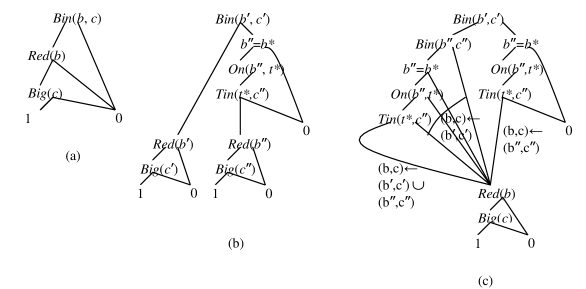
Figure 17: An example illustrating union or.

6.4 Object Maximization

Notice that since we are handling different probabilistic alternatives of the same action separately we must keep action parameters fixed during the regression process and until they are added in step $1$ of the algorithm. In step 2 we maximize over the choice of action parameters. As mentioned above we get this maximization for free. We simply rename the action parameters using new variable names (to avoid repetition between iterations) and consider them as variables. The aggregation semantics provides the maximization and by definition this selects the best instance of the action. Since constants are turned into variables additional reduction is typically possible at this stage. Any combination of weak and strong reductions can be used. From the discussion we have the following lemma:

Lemma 13

Consider any concrete instantiation of a RMDP. Let $V_{n}$ be a value function for the corresponding MDP, and let $A(\vec{x})$ be a probabilistic action in the domain. Then $Q_{V_{n}}^{A}$ as calculated by object maximization in step 2 of the algorithm is correct. That is, for any state $s$, ${\mbox{MAP}}_{Q_{V_{n}}^{A}}(s)$ is the maximum over expected values achievable by executing an instance of $A(\vec{x})$ in $s$ and then receiving the terminal value $V_{n}$.

A potential criticism of our object maximization is that we are essentially adding more variables to the diagram and thus future evaluation of the diagram in any state becomes more expensive (since more substitutions need to be considered). However, this is only true if the diagram remains unchanged after object maximization. In fact, as illustrated in the example given below, these variables may be pruned from the diagram in the process of reduction. Thus as long as the final value function is compact the evaluation is efficient and there is no such hidden cost.

6.5 Maximizing Over Actions

The maximization $V_{n+1}=\max_{A}Q_{n+1}^{A}$ in step (3) combines independent functions. Therefore as above we must first standardize apart the different diagrams, then we can follow with the propositional Apply procedure and finally follow with weak and strong reductions. This clearly maintains correctness for any concrete instantiation of the state space.

6.6 Order Over Argument Types

We can now resume the discussion of ordering of argument types and extend it to predicate and action parameters. As above, some structure is suggested by the operations of the algorithm. Section 3.5 already suggested that we order constants before variables.

Action parameters are “special constants” before object maximization but they become variables during object maximization. Thus their position should allow them to behave as variables. We should therefore also order constants before action parameters.

Note that predicate parameters only exist inside TVDs, and will be replaced with domain constants or variables during regression. Thus we only need to decide on the relative order between predicate parameters and action parameters. If we put action parameters before predicate parameters and the latter is replaced with a constant then we get an order violation, so this order is not useful. On the other hand, if we put predicate parameters before action parameters then both instantiations of predicate parameters are possible. Notice that when substituting a predicate parameter with a variable, action parameters still need to be larger than the variable (as they were in the TVD). Therefore, we also order action parameters after variables.

To summarize, the ordering: constants $\prec$ variables (predicate parameters in case of TVDs) $\prec$ action parameters, is suggested by heuristic considerations for orders that maximize the potential for reductions, and avoid the need for re-sorting diagrams.

Finally, note that if we want to maintain the diagram sorted at all times, we need to maintain variant versions of each TVD capturing possible ordering of replacements of predicate parameters. Consider a TVD in Figure 18(a). If we rename predicate parameters $X$ and $Y$ to be $x_{2}$ and $x_{1}$ respectively, and if $x_{1}\prec x_{2}$, then the resulting sub-FODD as shown in Figure 18(b) violates the order. To solve this problem we have to define another TVD corresponding to the case where the substitution of $X$ $\succ$ the substitution of $Y$, as shown in Figure 18(c). In the case of replacing $X$ with $x_{2}$ and $Y$ with $x_{1}$, we use the TVD in Figure 18(c) instead of the one in Figure 18(a).

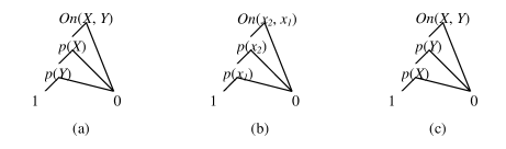
Figure 18: An example illustrating the necessity to maintain multiple TVDs.

6.7 Convergence and Complexity

Since each step of Procedure 1 is correct we have the following theorem:

Theorem 2

Consider any concrete instantiation of a RMDP. Let $V_{n}$ be the value function for the corresponding MDP when there are $n$ steps to go. Then the value of $V_{n+1}$ calculated by Procedure 1 correctly captures the value function when there are $n+1$ steps to go. That is, for any state $s$, ${\mbox{MAP}}_{V_{n+1}}(s)$ is the maximum expected value achievable in $s$ in $n+1$ steps.

Note that for RMDPs some problems require an infinite number of state partitions. Thus we cannot converge to $V^{*}$ in a finite number of steps. However, since our algorithm implements VI exactly, standard results about approximating optimal value functions and policies still hold. In particular the following standard result (?) holds for our algorithm, and our stopping criterion guarantees approximating optimal value functions and policies.

Theorem 3

Let $V^{*}$ be the optimal value function and let $V_{k}$ be the value function calculated by the relational VI algorithm.
(1) If $r(s)\leq M$ for all $s$ then $\|V_{n}-V^{*}\|\leq\varepsilon$ for $n\geq\frac{log(\frac{2M}{\varepsilon(1-\gamma)})}{log\frac{1}{\gamma}}$.
(2) If $\|V_{n+1}-V_{n}\|\leq\frac{\varepsilon(1-\gamma)}{2\gamma}$ then $\|V_{n+1}-V^{*}\|\leq\varepsilon$.

While the algorithm maintains compact diagrams, reduction of diagrams is not guaranteed for all domains. Therefore we can only provide trivial upper bounds in terms of worst case time complexity. Notice first that every time we use the Apply procedure the size of the output diagram may be as large as the product of the size of its inputs. We must also consider the size of the FODD giving the regressed value function. While Block replacement is $O(N)$ where $N$ is the size of the current value function, it is not sorted and sorting may require both exponential time and space in the worst case. For example, ? (?) illustrates how ordering may affect the size of a diagram. For a function of $2n$ arguments, the function $x_{1}\cdot x_{2}+x_{3}\cdot x_{4}+\cdots+x_{2n-1}\cdot x_{2n}$ only requires a diagram of $2n+2$ nodes, while the function $x_{1}\cdot x_{n+1}+x_{2}\cdot x_{n+2}+\cdots+x_{n}\cdot x_{2n}$ requires $2^{n+1}$ nodes. Notice that these two functions only differ by a permutation of their arguments. Now if $x_{1}\cdot x_{2}+x_{3}\cdot x_{4}+\cdots+x_{2n-1}\cdot x_{2n}$ is the result of block replacement then clearly sorting requires exponential time and space. The same is true for our block combination procedure or any other method of calculating the result, simply because the output is of exponential size. In such a case heuristics that change variable ordering, as in propositional ADDs (?), would probably be very useful.

Assuming TVDs, reward function, and probabilities all have size $\leq C$, each action has $\leq M$ action alternatives, the current value function $V_{n}$ has $N$ nodes, and worst case space expansion for regression and all Apply operations, the overall size of the result and the time complexity for one iteration are $O(C^{M^{2}(N+1)})$. However note that this is the worst case analysis and does not take reductions into account. While our method is not guaranteed to always work efficiently, the alternative of grounding the MDP will have an unmanageable number of states to deal with, so despite the high worst case complexity our method provides a potential improvement. As the next example illustrates, reductions can substantially decrease diagram size and therefore save considerable time in computation.

6.8 A Comprehensive Example of Value Iteration

Figure 19 traces steps in the application of value iteration to the logistics domain. The TVDs, action choice probabilities, and reward function for this domain are given in Figure 13. To simplify the presentation, we continue using the predicate ordering $Bin\prec$ “=” $\prec On\prec Tin\prec rain$ introduced earlier.

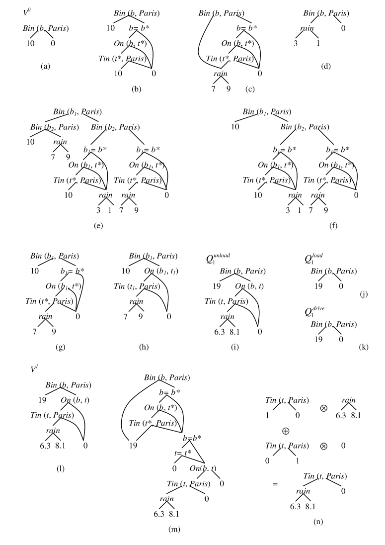
Figure 19: An example of value iteration in the Logistics Domain.

Given $V_{0}=R$ as shown in Figure 19(a), Figure 19(b) gives the result of regression of $V_{0}$ through $unloadS(b^{*},t^{*})$ by block replacement, denoted as $Regr(V_{0},unloadS(b^{*},t^{*}))$.

Figure 19(c) gives the result of multiplying $Regr(V_{0},unloadS(b^{*},t^{*}))$ with the choice probability of $unloadS$ $Pr(unloadS(b^{*},t^{*}))$.

Figure 19(d) gives the result of $Pr(unloadF(b^{*},t^{*}))\otimes Regr(V_{0},unloadF(b^{*},t^{*}))$. Notice that this diagram is simpler since $unloadF$ does not change the state and the TVDs for it are trivial.

Figure 19(e) gives the unreduced result of adding two outcomes for $unload(b^{*},t^{*})$, i.e., the result of adding $[Pr(unloadS(b^{*},t^{*}))\otimes Regr(V_{0},unloadS(b^{*},t^{*}))]$ to $[Pr(unloadF(b^{*},t^{*}))$ $\otimes Regr(V_{0},unloadF(b^{*},t^{*}))].$ Note that we first standardize apart diagrams for $unloadS(b^{*},t^{*})$ and $unloadF(b^{*},t^{*})$ by respectively renaming $b$ as $b_{1}$ and $b_{2}$. Action parameters $b^{*}$ and $t^{*}$ at this stage are considered as constants and we do not change them. Also note that the recursive part of Apply (addition $\oplus$) has performed some reductions, i.e., removing the node $rain$ when both of its children lead to value $10$.

In Figure 19(e), we can apply R6 to node $Bin(b_{2},Paris)$ in the left branch. The conditions
P7.1: $[\exists b_{1},Bin(b_{1},Paris)]\rightarrow[\exists b_{1},b_{2},Bin(b_{1},Paris)\wedge Bin(b_{2},Paris)]$,
V7.1: $min(Bin(b_{2},Paris)_{\downarrow t})=10\geq max(Bin(b_{2},Paris)_{\downarrow f})=9$,
V7.2: $Bin(b_{2},Paris)_{\downarrow t}$ is a constant
hold. According to Lemma 3 and Lemma 5 we can drop node $Bin(b_{2},Paris)$ and connect its parent $Bin(b_{1},Paris)$ to its true branch. Figure 19(f) gives the result after this reduction.

Next, consider the true child of $Bin(b_{2},Paris)$ and the true child of the root. The conditions
P7.1: $[\exists b_{1},b_{2},\neg Bin(b_{1},Paris)\wedge Bin(b_{2},Paris)]\rightarrow[\exists b_{1},Bin(b_{1},Paris)]$,
V7.1: $min(Bin(b_{1},Paris)_{\downarrow t})=10\geq max(Bin(b_{2},Paris)_{\downarrow t})=10$,
V7.2: $min(Bin(b_{1},Paris)_{\downarrow t})=10\geq max(Bin(b_{2},Paris)_{\downarrow f})=9$
hold. According to Lemma 3 and Lemma 5, we can drop the node $Bin(b_{2},Paris)$ and connect its parent $Bin(b_{1},Paris)$ to $Bin(b_{2},Paris)_{\downarrow f}$. Figure 19(g) gives the result after this reduction and now we get a fully reduced diagram. This is $T_{V_{0}}^{unload(b^{*},t^{*})}$.

In the next step we perform object maximization to maximize over action parameters $b^{*}$ and $t^{*}$ and get the best instance of the action $unload$. Note that $b^{*}$ and $t^{*}$ have now become variables, and we can perform one more reduction: we can drop the equality on the right branch by R9. Figure 19(h) gives the result after object maximization, i.e., $\mbox{obj-max}(T_{V_{0}}^{unload(b^{*},t^{*})})$. Note that we have renamed the action parameters to avoid the repetition between iterations.

Figure 19(i) gives the reduced result of multiplying Figure 19(h), $\mbox{obj-max}(T_{V_{0}}^{unload(b^{*},t^{*})})$, by $\gamma=0.9$, and adding the reward function. This result is $Q^{unload}_{1}$.

We can calculate $Q^{load}_{1}$ and $Q^{drive}_{1}$ in the same way and results are shown in Figure 19(j) and Figure 19(k) respectively. For $drive$ the TVDs are trivial and the calculation is relatively simple. For $load$, the potential loading of a box already in Paris is dropped from the diagram by the reduction operators in the process of object maximization.

Figure 19(l) gives $V_{1}$, the result after maximizing over $Q^{unload}_{1}$, $Q^{load}_{1}$ and $Q^{drive}_{1}$. Here again we standardized apart the diagrams, maximized over them, and then reduced the result. In this case the diagram for $unload$ dominates the other actions. Therefore $Q^{unload}_{1}$ becomes $V_{1}$, the value function after the first iteration.

Now we can start the second iteration, i.e., computing $V_{2}$ from $V_{1}$. Figure 19(m) gives the result of block replacement in regression of $V^{1}$ through action alternative $unloadS(b^{*},t^{*})$. Note that we have sorted the TVD for $on(B,T)$ so that it obeys the ordering we have chosen. However, the diagram resulting from block replacement is not sorted.

To address this we use the block combination algorithm to combine blocks bottom up. Figure 19(n) illustrates how we combine blocks $Tin(t,Paris)$, which is a TVD, and its two children, which have been processed and are general FODDs. After we combine $Tin(t,Paris)$ and its two children, $On(b,t)_{\downarrow t}$ has been processed. Since $On(b,t)_{\downarrow f}=0$, now we can combine $On(b,t)$ and its two children in the next step of block combination. Continuing this process we get a sorted representation of $Regr(V_{1},unloadS(b^{*},t^{*}))$.

6.9 Extracting Optimal Policies

There is more than one way to represent policies with FODDs. Here we simply note that a policy can be represented implicitly by a set of regressed value functions. After the value iteration terminates, we can perform one more iteration and compute the set of $Q$-functions using Equation 3.

Then, given a state $s$, we can compute the maximizing action as follows:

1. For each $Q$-function $Q^{A(\vec{x})}$, compute ${\mbox{MAP}}_{Q^{A(\vec{x})}}(s)$, where $\vec{x}$ are considered as variables.

2. For the maximum map obtained, record the action name and action parameters (from the valuation) to obtain the maximizing action.

This clearly implements the policy represented by the value function. An alternative approach that represents the policy explicitly was developed in the context of a policy iteration algorithm (?).

7 Discussion

ADDs have been used successfully to solve propositional factored MDPs. Our work gives one proposal of lifting these ideas to RMDPs. While the general steps are similar, the technical details are significantly more involved than the propositional case. Our decision diagram representation combines the strong points of the SDP and ReBel approaches to RMDP. On the one hand we get simple regression algorithms directly manipulating the diagrams. On the other hand we get object maximization for free as in ReBel. We also get space saving since different state partitions can share structure in the diagrams. A possible disadvantage compared to ReBel is that the reasoning required for reduction operators might be complex.

In terms of expressiveness, our approach can easily capture probabilistic STRIPS style formulations as in ReBel, allowing for more flexibility since we can use FODDs to capture rewards and transitions. For example, our representation can capture universal effects of actions. On the other hand, it is more limited than SDP since we cannot use arbitrary formulas for rewards, transitions, and probabilistic choice. For example we cannot express universal quantification using maximum aggregation, so these cannot be used in reward functions or in action preconditions. Our approach can also capture grid-world RL domains with state based reward (which are propositional) in factored form since the reward can be described as a function of location.

By contrasting the single path semantics with the multiple path semantics we see an interesting tension between the choice of representation and task. The multiple path method does not directly support state partitions, which makes it awkward to specify distributions and policies (since values and actions must both be specified at leaves). However, this semantics simplifies many steps by easily supporting disjunction and maximization over valuations which are crucial for for value iteration so it is likely to lead to significant saving in space and time.

An implementation and empirical evaluation are in progress. The precise choice of reduction operators and their application will be crucial to obtain an effective system, since in general there is a tradeoff between run time needed for reductions and the size of resulting FODDs. We can apply complex reduction operators to get the maximally reduced FODDs, but it takes longer to perform the reasoning required. This optimization is still an open issue both theoretically and empirically. Additionally, our implementation can easily incorporate the idea of approximation by combining leaves with similar values to control the size of FODDs (?). This gives a simple way of trading off efficiency against accuracy of the value functions.

There are many open issues concerning the current representation. Our results for FODDs give a first step toward a complete generalization of ADDs. Crucially we do not yet have a semantically appropriate normal form that is important in simplifying reasoning. While one can define a normal form (cf., ?, for a treatment of conjunctions) it is not clear if this can be calculated incrementally using local operations as in ADDs. It would be interesting to investigate conditions that guarantee a normal form for a useful set of reduction operators for FODDs.

Another possible improvement is that the representation can be modified to allow further compression. For example we can allow edges to rename variables when they are traversed so as to compress isomorphic sub-FODDs as illustrated above in Figure 17(c). Another interesting possibility is a copy operator that evaluates several copies of a predicate (with different variables) in the same node as illustrated in Figure 20. For such constructs to be usable one must modify the FODD and MDP algorithmic steps to handle diagrams with the new syntactic notation.

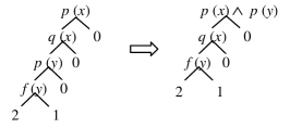
Figure 20: Example illustrating the copy operator.

8 Conclusion

The paper makes two main contributions. First, we introduce FODDs, a generalization of ADDs, for relational domains that may be useful in various applications. We have developed calculus of FODDs and reduction operators to minimize their size but there are many open issues regarding the best choice of operators and reductions. The second contribution is in developing a FODD-based value iteration algorithm for RMDPs that has the potential for significant improvement over previous approaches. The algorithm performs general relational probabilistic reasoning without ever grounding the domains and it is proved to converge to the abstract optimal value function when such a solution exists.

References

- Bahar, Frohm, Gaona, Hachtel, Macii, Pardo, and Somenzi Bahar, R. I., Frohm, E. A., Gaona, C. M., Hachtel, G. D., Macii, E., Pardo, A., and Somenzi, F. (1993). Algebraic decision diagrams and their applications. In Proceedings of the International Conference on Computer-Aided Design, pp. 188–191.
- Bellman Bellman, R. E. (1957). Dynamic programming. Princeton University Press.
- Blockeel and De Raedt Blockeel, H., and De Raedt, L. (1998). Top down induction of first order logical decision trees. Artificial Intelligence, 101, 285–297.
- Boutilier, Dean, and Goldszmidt Boutilier, C., Dean, T., and Goldszmidt, M. (2000). Stochastic dynamic programming with factored representations. Artificial Intelligence, 121(1), 49–107.
- Boutilier, Dean, and Hanks Boutilier, C., Dean, T., and Hanks, S. (1999). Decision-theoretic planning: Structural assumptions and computational leverage. Journal of Artificial Intelligence Research, 11, 1–94.
- Boutilier, Dearden, and Goldszmidt Boutilier, C., Dearden, R., and Goldszmidt, M. (1995). Exploiting structure in policy construction. In Proceedings of the International Joint Conference of Artificial Intelligence, pp. 1104–1111.
- Boutilier, Reiter, and Price Boutilier, C., Reiter, R., and Price, B. (2001). Symbolic dynamic programming for first-order MDP s. In Proceedings of the International Joint Conference of Artificial Intelligence, pp. 690–700.
- Bryant Bryant, R. E. (1986). Graph-based algorithms for boolean function manipulation. IEEE Transactions on Computers, C-35(8), 677–691.
- Bryant Bryant, R. E. (1992). Symbolic boolean manipulation with ordered binary decision diagrams. ACM Computing Surveys, 24(3), 293–318.
- Cormen, Leiserson, Rivest, and Stein Cormen, T. H., Leiserson, C. E., Rivest, R. L., and Stein, C. (2001). Introduction to Algorithms. MIT Press.
- Driessens, Ramon, and Gärtner Driessens, K., Ramon, J., and Gärtner, T. (2006). Graph kernels and gaussian processes for relational reinforcement learning. Machine Learning, 64(1-3), 91–119.
- Dzeroski, De Raedt, and Driessens Dzeroski, S., De Raedt, L., and Driessens, K. (2001). Relational reinforcement learning. Machine Learning, 43, 7–52.
- Feng and Hansen Feng, Z., and Hansen, E. A. (2002). Symbolic heuristic search for factored Markov Decision Processes. In Proceedings of the National Conference on Artificial Intelligence, pp. 455–460.
- Fern, Yoon, and Givan Fern, A., Yoon, S., and Givan, R. (2003). Approximate policy iteration with a policy language bias. In International Conference on Neural Information Processing Systems.
- Fern, Yoon, and Givan Fern, A., Yoon, S., and Givan, R. (2006). Approximate policy iteration with a policy language bias: Solving relational Markov Decision Processes. Journal of Artificial Intelligence Research, 25, 75–118.
- Garriga, Khardon, and De Raedt Garriga, G., Khardon, R., and De Raedt, L. (2007). On mining closed sets in multi-relational data. In Proceedings of the International Joint Conference of Artificial Intelligence, pp. 804–809.
- Gretton and Thiebaux Gretton, C., and Thiebaux, S. (2004). Exploiting first-order regression in inductive policy selection. In Proceedings of the Conference on Uncertainty in Artificial Intelligence, pp. 217–225.
- Groote and Tveretina Groote, J. F., and Tveretina, O. (2003). Binary decision diagrams for first-order predicate logic. The Journal of Logic and Algebraic Programming, 57, 1–22.
- Großmann, Hölldobler, and Skvortsova Großmann, A., Hölldobler, S., and Skvortsova, O. (2002). Symbolic dynamic programming within the fluent calculus. In Proceedings of the IASTED International Conference on Artificial and Computational Intelligence.
- Guestrin, Koller, Gearhart, and Kanodia Guestrin, C., Koller, D., Gearhart, C., and Kanodia, N. (2003a). Generalizing plans to new environments in relational MDPs. In Proceedings of the International Joint Conference of Artificial Intelligence, pp. 1003–1010.
- Guestrin, Koller, Par, and Venktaraman Guestrin, C., Koller, D., Par, R., and Venktaraman, S. (2003b). Efficient solution algorithms for factored MDPs. Journal of Artificial Intelligence Research, 19, 399–468.
- Hansen and Feng Hansen, E. A., and Feng, Z. (2000). Dynamic programming for POMDPs using a factored state representation. In Proceedings of the International Conference on Artificial Intelligence Planning Systems, pp. 130–139.
- Hoey, St-Aubin, Hu, and Boutilier Hoey, J., St-Aubin, R., Hu, A., and Boutilier, C. (1999). SPUDD: Stochastic planning using decision diagrams. In Proceedings of the Conference on Uncertainty in Artificial Intelligence, pp. 279–288.
- Höolldobler, Karabaev, and Skvortsova Höolldobler, S., Karabaev, E., and Skvortsova, O. (2006). FluCaP: a heuristic search planner for first-order MDPs. Journal of Artificial Intelligence Research, 27, 419–439.
- Kersting, Otterlo, and De Raedt Kersting, K., Otterlo, M. V., and De Raedt, L. (2004). Bellman goes relational. In Proceedings of the International Conference on Machine Learning.
- McMillan McMillan, K. L. (1993). Symbolic model checking. Kluwer Academic Publishers.
- Puterman Puterman, M. L. (1994). Markov decision processes: Discrete stochastic dynamic programming. Wiley.
- Rivest Rivest, R. L. (1987). Learning decision lists. Machine Learning, 2(3), 229–246.
- Sanghai, Domingos, and Weld Sanghai, S., Domingos, P., and Weld, D. (2005). Relational dynamic bayesian networks. Journal of Artificial Intelligence Research, 24, 759–797.
- Sanner and Boutilier Sanner, S., and Boutilier, C. (2005). Approximate linear programming for first-order MDPs. In Proceedings of the Conference on Uncertainty in Artificial Intelligence.
- Sanner and Boutilier Sanner, S., and Boutilier, C. (2006). Practical linear value-approximation techniques for first-order MDPs. In Proceedings of the Conference on Uncertainty in Artificial Intelligence.
- Sanner and Boutilier Sanner, S., and Boutilier, C. (2007). Approximate solution techniques for factored first-order MDPs. In Proceedings of the International Conference on Automated Planning and Scheduling.
- Schuurmans and Patrascu Schuurmans, D., and Patrascu, R. (2001). Direct value approximation for factored MDPs. In International Conference on Neural Information Processing Systems, pp. 1579–1586.
- St-Aubin, Hoey, and Boutilier St-Aubin, R., Hoey, J., and Boutilier, C. (2000). APRICODD: Approximate policy construction using decision diagrams. In International Conference on Neural Information Processing Systems, pp. 1089–1095.
- Wang Wang, C. (2007). First order Markov Decision Processes. Tech. rep. TR-2007-4, Computer Science Department, Tufts University.
- Wang, Joshi, and Khardon Wang, C., Joshi, S., and Khardon, R. (2007). First order decision diagrams for relational MDPs. In Proceedings of the International Joint Conference of Artificial Intelligence, pp. 1095–1100.
- Wang and Khardon Wang, C., and Khardon, R. (2007). Policy iteration for relational MDPs. In Proceedings of the Conference on Uncertainty in Artificial Intelligence.