The joint graphical lasso for inverse covariance estimation across multiple classes

Abstract

We consider the problem of estimating multiple related Gaussian graphical models from a high-dimensional data set with observations belonging to distinct classes. We propose the joint graphical lasso, which borrows strength across the classes in order to estimate multiple graphical models that share certain characteristics, such as the locations or weights of nonzero edges. Our approach is based upon maximizing a penalized log likelihood. We employ generalized fused lasso or group lasso penalties, and implement a fast ADMM algorithm to solve the corresponding convex optimization problems. The performance of the proposed method is illustrated through simulated and real data examples.

Keywords: alternating directions method of multipliers; generalized fused lasso; group lasso; graphical lasso; network estimation; Gaussian graphical model; high-dimensional

1 Introduction

In recent years, much interest has focused upon estimating an undirected graphical model on the basis of a $n\times p$ data matrix $\bf X$, where $n$ is the number of observations and $p$ is the number of features. Suppose that the observations ${\bf x}_{1},\ldots,{\bf x}_{n}\in\mathbb{R}^{p}$ are independent and identically distributed $N(\boldsymbol{\mu},{\bf\Sigma})$, where $\boldsymbol{\mu}\in\mathbb{R}^{p}$ and $\bf\Sigma$ is a positive definite $p\times p$ matrix. Then zeros in the inverse covariance matrix ${\bf\Sigma}^{-1}$ correspond to pairs of features that are conditionally independent – that is, pairs of variables that are independent of each other, given all of the other variables in the data set. In a Gaussian graphical model (Lauritzen, 1996), these conditional dependence relationships are represented by a graph in which nodes represent features and edges connect conditionally dependent pairs of features.

A natural way to estimate the precision (or concentration) matrix ${\bf\Sigma}^{-1}$ is via maximum likelihood. Letting $\bf S$ denote the empirical covariance matrix of $\bf X$, the Gaussian log likelihood takes the form (up to a constant)

$$\frac{n}{2}\left(\log\det{{\bf\Sigma}^{-1}}-\mathrm{trace}({\bf S}{{\bf\Sigma}^{-1}})\right).$$ (1.1)

Maximizing (1.1) with respect to ${\bf\Sigma}^{-1}$ yields the maximum likelihood estimate ${\bf S}^{-1}$.

However, two problems can arise in using this maximum likelihood approach to estimate ${\bf\Sigma}^{-1}$. First, in the high-dimensional setting where the number of features $p$ is larger than the number of observations $n$, the empirical covariance matrix $\bf S$ is singular and so cannot be inverted to yield an estimate of ${\bf\Sigma}^{-1}$. If $p\approx n$, then even if $\bf S$ is not singular, the maximum likelihood estimate for ${\bf\Sigma}^{-1}$ will suffer from very high variance. Second, one often is interested in identifying pairs of variables that are unconnected in the graphical model, i.e. that are conditionally independent; these correspond to zeros in ${\bf\Sigma}^{-1}$. But maximizing the log likelihood (1.1) will in general yield an estimate of ${\bf\Sigma}^{-1}$ with no elements that are exactly equal to zero.

In recent years, a number of proposals have been made for estimating ${\bf\Sigma}^{-1}$ in the high-dimensional setting in such a way that the resulting estimate is sparse. Meinshausen & Bühlmann (2006) proposed doing this via a penalized regression approach, which was extended by Peng et al. (2009). A number of authors have instead taken a penalized log likelihood approach (Yuan & Lin, 2007b; Friedman, Hastie & Tibshirani, 2007; Rothman et al., 2008): rather than maximizing (1.1), one can instead solve the problem

$$\mathrm{maximize}_{{\bf\Theta}}\left\{\log\det{\bf\Theta}-\mathrm{trace}({\bf S}{\bf\Theta})-\lambda||{\bf\Theta}||_{1}\right\},$$ (1.2)

where $\lambda$ is a nonnegative tuning parameter. The solution to this optimization problem provides an estimate for ${\bf\Sigma}^{-1}$. The use of an $\ell_{1}$ or lasso (Tibshirani, 1996) penalty on the elements of ${\bf\Theta}$ has the effect that when the tuning parameter $\lambda$ is large, some elements of the resulting precision matrix estimate will be exactly equal to zero. Moreover, (1.2) can be solved even if $p\gg n$. The solution to the problem (1.2) is referred to as the graphical lasso. Some authors have proposed applying the $\ell_{1}$ penalty in (1.2) only to the off-diagonal elements of $\bf\Theta$.

Graphical models are especially of interest in the analysis of gene expression data, since it is believed that genes operate in pathways, or networks. Graphical models based on gene expression data can provide a useful tool for visualizing the relationships among genes and for generating biological hypotheses. The standard formulation for estimating a Gaussian graphical model assumes that each observation is drawn from the same distribution. However, in many datasets the observations may correspond to several distinct classes, so the assumption that all observations are drawn from the same distribution is inappropriate. For instance, suppose that a cancer researcher collects gene expression measurements for a set of cancer tissue samples and a set of normal tissue samples. In this case, one might want to estimate a graphical model for the cancer samples and a graphical model for the normal samples. One would expect the two graphical models to be similar to each other, since both are based upon the same type of tissue, but also to have important differences stemming from the fact that gene networks are often dysregulated in cancer. Estimating separate graphical models for the cancer and normal samples does not exploit the similarity between the true graphical models. And estimating a single graphical model for the cancer and normal samples ignores the fact that we do not expect the true graphical models to be identical, and that the differences between the graphical models may be of interest.

In this paper, we propose the joint graphical lasso, a technique for jointly estimating multiple graphical models corresponding to distinct but related conditions, such as cancer and normal tissue. Our approach is an extension of the graphical lasso (1.2) to the case of multiple data sets. It is based upon a penalized log likelihood approach, where the choice of penalty depends on the characteristics of the graphical models that we expect to be shared across conditions.

We illustrate our method with a small toy example that consists of observations from two classes. Within each class, the observations are independent and identically distributed according to a normal distribution. The two classes have distinct covariance matrices. When we apply the graphical lasso separately to the observations in each class, the resulting graphical model estimates are less accurate than when we use our joint graphical lasso approach. Results are shown in Figure 1.

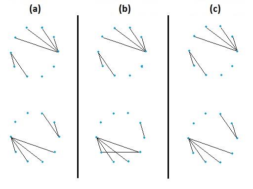
Figure 1: Comparison of the graphical lasso with our joint graphical lasso in a toy example with two conditions, $p=10$ variables, and n=200 observations per condition. (a): True networks. (b): Networks estimated by applying the graphical lasso separately to each class. (c): Networks estimated by applying our joint graphical lasso proposal.

The rest of this paper is organized as follows. In Section 2, we present the joint graphical lasso optimization problem. Section 3 contains an alternating directions method of multipliers algorithm for its solution. In Section 4, we present theoretical results that lead to massive gains in the algorithm’s computational efficiency. Section 5 contains a discussion of related approaches from the literature, and in Section 6 we discuss tuning parameter selection. In Section 7, we illustrate the performance of our proposal in a simulation study. Section 8 contains an application to a lung cancer gene expression dataset. The discussion is in Section 9.

2 The joint graphical lasso

We briefly introduce some notation that will be used throughout this paper.

We let $K$ denote the number of classes in our data, and let ${\bf\Sigma}^{-1}_{k}$ denote the true precision matrix for the $k$th class. We will seek to estimate ${\bf\Sigma}^{-1}_{1},\ldots,{\bf\Sigma}^{-1}_{K}$ by formulating convex optimization problems with arguments $\{{\bf\Theta}\}={\bf\Theta}^{(1)},\ldots,{\bf\Theta}^{(K)}$. The solutions $\hat{{\bf\Theta}}^{(1)},\ldots,\hat{{\bf\Theta}}^{(K)}$ to these optimization problems will constitute estimates of ${\bf\Sigma}^{-1}_{1},\ldots,{\bf\Sigma}^{-1}_{K}$.

We will index matrix elements using $i=1,\ldots,p$, $j=1,\ldots,p$, and will index classes using $k=1,\ldots,K$. $\|{\bf A}\|_{F}$ will denote the Frobenius norm of matrix ${\bf A}$, i.e. $\|{\bf A}\|_{F}=\sqrt{\sum_{i}\sum_{j}A_{ij}^{2}}$ .

2.1 The general formulation for the joint graphical lasso

Suppose that we are given $K$ data sets, ${\bf Y}^{(1)},\ldots,{\bf Y}^{(K)}$, with $K\geq 2$. ${\bf Y}^{(k)}$ is a $n_{k}\times p$ matrix consisting of $n_{k}$ observations with measurements on a set of $p$ features, which are common to all $K$ data sets. Furthermore, we assume that the $\sum_{k=1}^{K}n_{k}$ observations are independent, and that the observations within each data set are identically distributed: ${\bf y}_{1}^{(k)},\ldots,{\bf y}_{n_{k}}^{(k)}\sim N(\boldsymbol{\mu}_{k},{\bf\Sigma}_{k})$. Without loss of generality, we assume that the features within each data set are centered such that $\boldsymbol{\mu}_{k}={\bf 0}$. We let ${\bf S}^{(k)}=\frac{1}{n_{k}}({\bf Y}^{(k)})^{T}{\bf Y}^{(k)}$, the empirical covariance matrix for ${\bf Y}^{(k)}$. The log likelihood for the data takes the form (up to a constant)

$$\ell({\{{\bf\Theta}\}})=\frac{1}{2}\sum_{k=1}^{K}n_{k}\left(\log\det{\bf\Theta}^{(k)}-\mathrm{trace}({\bf S}^{(k)}{\bf\Theta}^{(k)})\right).$$ (2.3)

Maximizing (2.3) with respect to ${\bf\Theta}^{(1)},\ldots,{\bf\Theta}^{(K)}$ yields the maximum likelihood estimate $({\bf S}^{(1)})^{-1},\ldots,({\bf S}^{(K)})^{-1}$.

However, depending on the application, the maximum likelihood estimates that result from (2.3) may not be satisfactory. When $p$ is smaller than but close to $n_{k}$, the maximum likelihood estimate can have very high variance, and no elements of $({\bf S}^{(1)})^{-1},\ldots,({\bf S}^{(K)})^{-1}$ will be zero, leading to difficulties in interpretation. In addition, when $p>n_{k}$, the maximum likelihood estimate becomes ill-defined. Moreover, if the $K$ data sets correspond to observations collected from $K$ distinct but related classes, then one might wish to borrow strength across the $K$ classes to estimate the $K$ precision matrices, rather than estimating each precision matrix separately.

Therefore, instead of estimating ${\bf\Sigma}^{-1}_{1},\ldots,{{\bf\Sigma}^{-1}_{K}}$ by maximizing (2.3), we consider the penalized log likelihood and seek $\{\hat{{\bf\Theta}}\}$ solving

$$\mathrm{maximize}_{\{{\bf\Theta}\}}\left\{\sum_{k=1}^{K}n_{k}\left(\log\det{{\bf\Theta}}^{(k)}-\mathrm{trace}\left({\bf S}^{(k)}{{\bf\Theta}}^{(k)}\right)\right)-P(\{{\bf\Theta}\})\right\}$$ (2.4)

subject to the constraint that ${\bf\Theta}^{(1)},\ldots,{\bf\Theta}^{(K)}$ are positive definite. Here $P(\{{\bf\Theta}\})$ denotes a convex penalty function, so that the objective in (2.4) is strictly concave in $\{{\bf\Theta}\}$. We propose to choose a penalty function $P$ that will encourage ${\hat{{\bf\Theta}}}^{(1)},\ldots,{\hat{{\bf\Theta}}}^{(K)}$ to share certain characteristics, such as the locations or values of the nonzero elements; moreover, we would like the estimated precision matrices to be sparse. In particular, we will consider penalty functions that take the form $P(\{{\bf\Theta}\})=\tilde{P}(\{{\bf\Theta}\})+\lambda_{1}\sum_{k}\sum_{i\neq j}|\theta^{(k)}_{ij}|$, where $\tilde{P}$ is a convex function and $\lambda_{1}$ is a nonnegative tuning parameter. When $\tilde{P}(\{{\bf\Theta}\})=0$, (2.4) amounts to performing $K$ uncoupled graphical lasso optimization problems (1.2). The $\tilde{P}$ penalty is chosen to encourage similarity across the $K$ estimated precision matrices; therefore, we refer to the solution to (2.4) as the joint graphical lasso (JGL). We discuss specific forms of the penalty function in (2.4) in the next section.

2.2 Two useful penalty functions

In this subsection, we introduce two particular choices of the convex penalty function $P$ in (2.4) that lead to useful graphical model estimates. In Appendix 1, we further extend these proposals to work on the scale of partial correlations.

2.2.1 The fused graphical lasso

The fused graphical lasso (FGL) is the solution to the problem (2.4) with the penalty

$$P(\{{\bf\Theta}\})=\lambda_{1}\sum_{k=1}^{K}\sum_{i\neq j}|\theta^{(k)}_{ij}|+\lambda_{2}\sum_{k<k^{\prime}}\sum_{i,j}|\theta^{(k)}_{ij}-\theta^{(k^{\prime})}_{ij}|,$$ (2.5)

where $\lambda_{1}$ and $\lambda_{2}$ are nonnegative tuning parameters. This is a generalized fused lasso penalty (Hoefling, 2010b), and results from applying $\ell_{1}$ penalties to (1) each off-diagonal element of the $K$ precision matrices, and (2) differences between corresponding elements of each pair of precision matrices. Like the graphical lasso, FGL results in sparse estimates $\hat{{\bf\Theta}}^{(1)},\ldots,\hat{{\bf\Theta}}^{(K)}$ when the tuning parameter $\lambda_{1}$ is large. In addition, many elements of $\hat{{\bf\Theta}}^{(1)},\ldots,\hat{{\bf\Theta}}^{(K)}$ will be identical across classes when the tuning parameter $\lambda_{2}$ is large (Tibshirani et al., 2005). Thus FGL borrows information aggressively across classes, encouraging not only similar network structure but also similar edge values.

2.2.2 The group graphical lasso

We define the group graphical lasso (GGL) to be the solution to (2.4) with

$$P(\{{\bf\Theta}\})=\lambda_{1}\sum_{k=1}^{K}\sum_{i\neq j}|\theta^{(k)}_{ij}|+\lambda_{2}\sum_{i\neq j}\sqrt{\sum_{k=1}^{K}{\theta^{(k)}_{ij}}^{2}}.$$ (2.6)

Again, $\lambda_{1}$ and $\lambda_{2}$ are nonnegative tuning parameters. A lasso penalty is applied to the elements of the precision matrices and a group lasso penalty is applied to the $(i,j)$ element across all $K$ precision matrices (Yuan & Lin, 2007a). This group lasso penalty encourages a similar pattern of sparsity across all of the precision matrices – that is, there will be a tendency for the zeros in the $K$ estimated precision matrices to occur in the same places. Specifically, when $\lambda_{1}=0$ and $\lambda_{2}>0$, each $\hat{{\bf\Theta}}^{(k)}$ will have an identical pattern of non-zero elements. On the other hand, the lasso penalty encourages further sparsity within each $\hat{{\bf\Theta}}^{(k)}$.

GGL encourages a weaker form of similarity across the $K$ precision matrices than does FGL: the latter encourages shared edge values across the $K$ matrices, whereas the former encourages only a shared pattern of sparsity.

3 Algorithm for the joint graphical lasso problem

3.1 An ADMM algorithm

We solve the problem (2.4) using an alternating directions method of multipliers (ADMM) algorithm. We refer the reader to Boyd et al. (2010) for a thorough exposition of ADMM algorithms as well as their convergence properties, and to Simon & Tibshirani (2012) and Mohan et al. (2012) for recent applications of ADMM to related problems.

To solve the problem (2.4) subject to the constraint that ${\bf\Theta}^{(k)}$ is positive definite for $k=1,\ldots,K$ using ADMM, we note that the problem can be rewritten as

$$\operatornamewithlimits{minimize}_{\{{\bf\Theta}\},\{{\bf Z}\}}\left\{-\sum_{k=1}^{K}n_{k}\left(\log\det{\bf\Theta}^{(k)}-\mathrm{trace}({\bf S}^{(k)}{\bf\Theta}^{(k)})\right)+P(\{{\bf Z}\})\right\},$$ (3.7)

subject to the positive-definiteness constraint as well as the constraint that ${\bf Z}^{(k)}={\bf\Theta}^{(k)}$ for $k=1,\ldots,K$, where $\{{\bf Z}\}=\{{{\bf Z}^{(1)}},\ldots,{\bf Z}^{(K)}\}$. The scaled augmented Lagrangian (Boyd et al., 2010) for this problem is given by

$$L_{\rho}(\{{\bf\Theta}\},\{{\bf Z}\},\{{\bf U}\})= - \sum_{k=1}^{K}n_{k}\left(\log\det{\bf\Theta}^{(k)}-\mathrm{trace}({\bf S}^{(k)}{\bf\Theta}^{(k)})\right)+P(\{{\bf Z}\})$$ (3.8)

$$+ \frac{\rho}{2}\sum_{k=1}^{K}||{\bf\Theta}^{(k)}-{\bf Z}^{(k)}+{\bf U}^{(k)}||_{F}^{2},$$

where $\{{\bf U}\}=\{{{\bf U}^{(1)}},\ldots,{\bf U}^{(K)}\}$ are dual variables. Roughly speaking, an ADMM algorithm corresponding to (3.8) results from iterating three simple steps. At the $i$th iteration, they are as follows:

1. $\{{\bf\Theta}_{(i)}\}\leftarrow\arg\min_{\{{\bf\Theta}\}}\left\{L_{\rho}\left(\{{\bf\Theta}\},\{{\bf Z}_{(i-1)}\},\{{\bf U}_{(i-1)}\}\right)\right\}$.

2. $\{{\bf Z}_{(i)}\}\leftarrow\arg\min_{\{{\bf Z}\}}\left\{L_{\rho}\left(\{{\bf\Theta}_{(i)}\},\{{\bf Z}\},\{{\bf U}_{(i-1)}\}\right)\right\}$.

3. $\{{\bf U}_{(i)}\}\leftarrow\{{\bf U}_{(i-1)}\}+(\{{\bf\Theta}_{(i)}\}-\{{\bf Z}_{(i)}\})$.

We now present the ADMM algorithm in greater detail.

ADMM algorithm for solving the joint graphical lasso problem

1. Initialize the variables: ${\bf\Theta}^{(k)}={\bf I}$, ${\bf U}^{(k)}={\bf 0}$, ${\bf Z}^{(k)}={\bf 0}$ for $k=1,\ldots,K$.

2. Select a scalar $\rho>0$.

3. For $i=1,2,3,\ldots$ until convergence:

   1. For $k=1,\ldots,K$, update ${\bf\Theta}_{(i)}^{(k)}$ as the minimizer (with respect to ${\bf\Theta}^{(k)}$) of

      $$-n_{k}\left(\log\det{\bf\Theta}^{(k)}-\mathrm{trace}({\bf S}^{(k)}{\bf\Theta}^{(k)})\right)+\frac{\rho}{2}||{\bf\Theta}^{(k)}-{\bf Z}_{(i-1)}^{(k)}+{\bf U}_{(i-1)}^{(k)}||_{F}^{2}.$$

      Letting ${\bf V}{\bf D}{\bf V}^{T}$ denote the eigendecomposition of ${\bf S}^{(k)}-{\rho}{\bf Z}_{(i-1)}^{(k)}/n_{k}+{\rho}{\bf U}_{(i-1)}^{(k)}/n_{k}$, the solution is given (Witten & Tibshirani, 2009) by ${\bf V}\tilde{\bf D}{\bf V}^{T}$, where $\tilde{\bf D}$ is the diagonal matrix with $j$th diagonal element

      $$\frac{n_{k}}{2\rho}\left(-D_{jj}+\sqrt{D_{jj}^{2}+4\rho/n_{k}}\right).$$

   2. Update $\{{\bf Z}_{(i)}\}$ as the minimizer (with respect to $\{{\bf Z}\}$) of

      $$\frac{\rho}{2}\sum_{k=1}^{K}||{\bf Z}^{(k)}-({\bf\Theta}_{(i)}^{(k)}+{\bf U}_{(i-1)}^{(k)})||_{F}^{2}+P(\{{\bf Z}\}).$$ (3.9)

   3. For $k=1,\ldots,K$, update ${\bf U}_{(i)}^{(k)}$ as ${\bf U}_{(i-1)}^{(k)}+({\bf\Theta}_{(i)}^{(k)}-{\bf Z}_{(i)}^{(k)})$.

The final $\hat{\bf\Theta}^{(1)},\ldots,\hat{\bf\Theta}^{(K)}$ that result from this algorithm are the JGL estimates of ${\bf\Sigma}^{-1}_{1},\ldots,{\bf\Sigma}^{-1}_{K}$. This algorithm is guaranteed to converge to the global optimum (Boyd et al., 2010). We note that the positive-definiteness constraint on the estimated precision matrices is naturally enforced by the update in Step (c)(i).

Details of the minimization of (3.9) will depend on the form of the convex penalty function $P$. We note that the task of minimizing (3.9) can be re-written as

$$\operatornamewithlimits{minimize}_{\{{\bf Z}\}}\left\{\frac{\rho}{2}\sum_{k=1}^{K}||{\bf Z}^{(k)}-{\bf A}^{(k)}||_{F}^{2}+P(\{{\bf Z}\})\right\},$$ (3.10)

where

$${\bf A}^{(k)}={\bf\Theta}_{(i)}^{(k)}+{\bf Y}_{(i-1)}^{(k)}.$$ (3.11)

We will see in Section 3.2 that for the FGL and GGL penalties, solving (3.10) is a simple task, regardless of the value of $K$.

The algorithm given above involves computing the eigen decomposition of a $p\times p$ matrix, which can be computationally demanding when $p$ is large. However, in Section 4, we will present two theorems that reveal that when the values of the tuning parameters $\lambda_{1}$ and $\lambda_{2}$ are large, one can obtain the exact solution to the JGL optimization problem without ever computing the eigen decomposition of a $p\times p$ matrix. Therefore, solving the JGL problem is fast even when $p$ is quite large. In Section 8, we will see that one can perform FGL with $K=2$ classes and almost 18,000 features in under 2 minutes.

3.2 Solving (3.10) for the joint graphical lasso

We now consider the problem of solving (3.10) if $P$ is a generalized fused lasso or group lasso penalty.

3.2.1 Solving (3.10) for FGL

If $P$ is the penalty given in (2.5), then (3.10) takes the form

$$\operatornamewithlimits{minimize}_{\{{\bf Z}\}}\left\{\frac{\rho}{2}\sum_{k=1}^{K}||{\bf Z}^{(k)}-{\bf A}^{(k)}||_{F}^{2}+\lambda_{1}\sum_{k=1}^{K}\sum_{i\neq j}|Z^{(k)}_{ij}|+\lambda_{2}\sum_{k<k^{\prime}}\sum_{i,j}|Z^{(k)}_{ij}-Z^{(k^{\prime})}_{ij}|\right\}.$$ (3.12)

Now (3.12) is completely separable with respect to each pair of matrix elements $(i,j)$: that is, one can simply solve, for each $(i,j)$,

$$\operatornamewithlimits{minimize}_{Z_{ij}^{(1)},\ldots,Z_{ij}^{(K)}}\left\{\frac{\rho}{2}\sum_{k=1}^{K}(Z_{ij}^{(k)}-{A}_{ij}^{(k)})^{2}+\lambda_{1}1_{i\neq j}\sum_{k=1}^{K}|Z^{(k)}_{ij}|+\lambda_{2}\sum_{k<k^{\prime}}|Z^{(k)}_{ij}-Z^{(k^{\prime})}_{ij}|\right\}.$$ (3.13)

This is a special case of the fused lasso signal approximator (Hoefling, 2010b) in which there is a fusion between each pair of variables. A very efficient algorithm for this special case, which can be performed in $O(K\log K)$ operations, is available (Hocking et al., 2011; Hoefling, 2010a; Tibshirani, 2012).

In fact, when $K=2$, (3.13) has a very simple closed form solution. When $\lambda_{1}=0$, it is easy to verify that the solution to (3.13) takes the form

$$(\hat{Z}_{ij}^{(1)},\hat{Z}_{ij}^{(2)})=\left\{\begin{array}[]{lll}(A_{ij}^{(1)}-\lambda_{2}/\rho,A_{ij}^{(2)}+\lambda_{2}/\rho)&\mbox{if $A_{ij}^{(1)}>A_{ij}^{(2)}+2\lambda_{2}/\rho$}\\ (A_{ij}^{(1)}+\lambda_{2}/\rho,A_{ij}^{(2)}-\lambda_{2}/\rho)&\mbox{if $A_{ij}^{(2)}>A_{ij}^{(1)}+2\lambda_{2}/\rho$}\\ (\frac{A_{ij}^{(1)}+A_{ij}^{(2)}}{2},\frac{A_{ij}^{(1)}+A_{ij}^{(2)}}{2})&\mbox{if $|A_{ij}^{(1)}-A_{ij}^{(2)}|\leq 2\lambda_{2}/\rho$}\\ \end{array}.\right.$$ (3.14)

And when $\lambda_{1}>0$, the solution to (3.13) can be obtained through soft-thresholding (3.14) by $\lambda_{1}/\rho$ (see Friedman, Hastie, Hoefling & Tibshirani, 2007). Here the soft-thresholding operator is defined as $S(x,c)=\mathrm{sgn}(x)(|x|-c)_{+}$, where $a_{+}=\max(a,0)$.

3.2.2 Solving (3.10) for GGL

If $P$ is the group lasso penalty (2.6), then (3.10) takes the form

$$\operatornamewithlimits{minimize}_{\{{\bf Z}\}}\left\{\frac{\rho}{2}\sum_{k=1}^{K}||{\bf Z}^{(k)}-{\bf A}^{(k)}||_{F}^{2}+\lambda_{1}\sum_{k=1}^{K}\sum_{i\neq j}|Z^{(k)}_{ij}|+\lambda_{2}\sum_{i\neq j}\sqrt{\sum_{k}{Z^{(k)}_{ij}}^{2}}\right\}.$$ (3.15)

First, for all $i=1,\ldots,p$ and $k=1,\ldots,K$, it is easy to see that the solution to (3.15) has $\hat{Z}^{(k)}_{ii}=A^{(k)}_{ii}$. And one can show that the off-diagonal elements take the form (Friedman et al., 2010)

$$\hat{Z}^{(k)}_{ij}=S(A^{(k)}_{ij},\lambda_{1}/\rho)\left(1-\frac{\lambda_{2}}{\rho\sqrt{\sum_{k=1}^{K}S(A^{(k)}_{ij},\lambda_{1}/\rho)^{2}}}\right)_{+},$$ (3.16)

where $S$ denotes the soft-thresholding operator.

4 Faster computations for FGL and GGL

We now present two theorems that lead to substantial computational improvements to the JGL algorithm presented in Section 3. Using these theorems, one can inspect the empirical covariance matrices ${\bf S}^{(1)},\ldots,{\bf S}^{(K)}$ in order to determine whether the solution to the JGL optimization problem is block diagonal after some permutation of the features. Then one can simply perform the JGL algorithm on the features within each block separately, in order to obtain exactly the same solution that would have been obtained by applying the algorithm to all $p$ features. This leads to huge speed improvements since it obviates the need to ever compute the eigen decomposition of a $p\times p$ matrix. Our results mirror recent improvements in algorithms for solving the graphical lasso problem (Witten et al., 2011; Mazumder & Hastie, 2012).

For instance, suppose that for a given choice of $\lambda_{1}$ and $\lambda_{2}$, we determine that the estimated inverse covariance matrices $\hat{\bf\Theta}^{(1)},\ldots,\hat{\bf\Theta}^{(K)}$ are block diagonal, each with the same $R$ blocks, the $r$th of which contains $p_{r}$ features, $\sum_{r=1}^{R}p_{r}=p$. Then in each iteration of the JGL algorithm, rather than having to compute the eigen decomposition of $K$ $p\times p$ matrices, we need only compute eigen decompositions of matrices of dimension $p_{1}\times p_{1},\ldots,p_{R}\times p_{R}$. This leads to a potentially massive reduction in computational complexity from $O(p^{3})$ to $\sum_{r=1}^{R}O(p_{r}^{3})$.

We begin with a very simple lemma for which the proof follows by inspection of (2.4). The lemma can be extended by induction to any number of blocks.

Lemma 4.1.

Suppose that the solution to the FGL or GGL optimization problem is block diagonal with known blocks. That is, the features can be reordered in such a way that each estimated inverse covariance matrix takes the form

$$\hat{{\bf\Theta}}^{(k)}=\left(\begin{array}[]{cc}\hat{{\bf\Theta}}^{(k)}_{1}&0\\ 0&\hat{{\bf\Theta}}^{(k)}_{2}\end{array}\right)$$ (4.17)

where each of $\hat{{\bf\Theta}}^{(1)}_{1},\ldots,\hat{{\bf\Theta}}^{(K)}_{1}$ has the same dimension. Then, $\hat{{\bf\Theta}}^{(1)}_{1},\ldots,\hat{{\bf\Theta}}^{(K)}_{1}$ and $\hat{{\bf\Theta}}^{(1)}_{2},\ldots,\hat{{\bf\Theta}}^{(K)}_{2}$ can be obtained by solving the FGL or GGL optimization problem on just the corresponding set of features.

We now present the key results. Theorems 1 and 2 outline necessary and sufficient conditions for the presence of block diagonal structure in the FGL and GGL optimization problems, and are proven in Appendix 2.

Theorem 1.

Consider the FGL optimization problem with $K=2$ classes. Let $C_{1}$ and $C_{2}$ be a non-overlapping partition of the $p$ variables such that $C_{1}\cap C_{2}=\emptyset$, $C_{1}\cup C_{2}=\{1,\ldots,p\}$. The following conditions are necessary and sufficient for the variables in $C_{1}$ to be completely disconnected from those in $C_{2}$ in each of the resulting network estimates:

1. $|n_{1}S^{(1)}_{ij}|\leq\lambda_{1}+\lambda_{2}$ for all $i\in C_{1}$ and $j\in C_{2}$,

2. $|n_{2}S^{(2)}_{ij}|\leq\lambda_{1}+\lambda_{2}$ for all $i\in C_{1}$ and $j\in C_{2}$, and

3. $|n_{1}S^{(1)}_{ij}+n_{2}S^{(2)}_{ij}|\leq 2\lambda_{1}$ for all $i\in C_{1}$ and $j\in C_{2}$.

Furthermore, if $K>2$, then

$$|n_{k}S^{(k)}_{ij}|\leq\lambda_{1}\mathrm{\;\;for\;all\;\;}i\in C_{1},\;j\in C_{2},\;k=1,\ldots,K$$ (4.18)

is a sufficient condition for the variables in $C_{1}$ to be completely disconnected from those in $C_{2}$.

Theorem 2.

Consider the GGL optimization problem with $K\geq 2$ classes. Let $C_{1}$ and $C_{2}$ be a non-overlapping partition of the $p$ variables, such that $C_{1}\cap C_{2}=\emptyset$, $C_{1}\cup C_{2}=\{1,\ldots,p\}$. The following condition is necessary and sufficient for the variables in $C_{1}$ to be completely disconnected from those in $C_{2}$ in each of the resulting network estimates:

$$\sum_{k=1}^{K}(|n_{k}S^{(k)}_{ij}|-\lambda_{1})_{+}^{2}\leq\lambda_{2}^{2}\mathrm{\;\;for\;all\;\;}i\in C_{1},\;j\in C_{2}\;.$$ (4.19)

Theorems 1 and 2 allow us to quickly check if, given a partition of the features $C_{1}$ and $C_{2}$, the solution to the JGL optimization problem is block diagonal with one block corresponding to features in $C_{1}$ and one block corresponding to features in $C_{2}$. In practice, for any given $(\lambda_{1},\lambda_{2})$, we can quickly perform the following two-step procedure to identify any block structure in the FGL or GGL solution:

1. Create $\bf M$, a $p\times p$ matrix with $M_{ii}=1$ for $i=1,\ldots,p$. For $i\neq j$, let $M_{ij}=0$ if the conditions specified in Theorem 1 are met for that pair of variables and the FGL penalty is used, or if the condition of Theorem 2 is met for that pair of variables and the GGL penalty is used. Otherwise, set $M_{ij}=1$.

2. Identify the connected components of the undirected graph whose adjacency matrix is given by $\bf M$. Note that this can be performed in $O(|M|)$ operations, where $|M|$ is the number of nonzero elements in $\bf M$ (Tarjan, 1972).

Theorems 1 and 2 guarantee that the connected components identified in Step (b) correspond to distinct blocks in the FGL or GGL solutions. Therefore, one can quickly obtain these solutions by solving the FGL or GGL optimization problems on the submatrices of these $K$ $p\times p$ empirical covariance matrices that correspond to that block diagonal structure. Consequently, we can obtain the exact solution to the JGL optimization problem on extremely high-dimensional data sets that would otherwise be computationally intractable. For instance, in Section 8 we performed FGL on a gene expression data set with almost $18,000$ features in under two minutes.

As pointed out by a reviewer, Theorems 1 and 2 lead to speed improvements only if the tuning parameters $\lambda_{1}$ and $\lambda_{2}$ are sufficiently large. We argue that this will in fact be the case in most practical applications of JGL. When network estimation is performed for the sake of data exploration and when $p$ is large, only a very sparse network estimate will be useful; otherwise, interpretation of the estimate will be impossible. Even when data exploration is not the end goal of the analysis, large values of $\lambda_{1}$ and $\lambda_{2}$ will generally be used, since most data sets cannot reasonably support estimation of $Kp(p+1)/2$ nonzero parameters when $n\ll p$.

5 Relationship to previous proposals

Several past proposals have been made to jointly estimate graphical models on the basis of observations drawn from distinct conditions. Some proposals have used time-series data to define time-varying networks in the context of continuous or binary data (Zhou et al., 2008; Song et al., 2009a; Ahmed & Xing, 2009; Kolar & Xing, 2009; Song et al., 2009b; Kolar et al., 2010). Guo et al. (2011) instead describe a likelihood-based method for estimating precision matrices across multiple related classes simultaneously. They employ a hierarchical penalty that forces similar patterns of sparsity across classes, an approach that is similar in spirit to GGL.

Our FGL and GGL proposals have a number of advantages over these existing approaches. Methods for estimating time-varying networks cannot be easily extended to the setting where the classes lack a natural ordering. Guo et al. (2011)’s proposal is a closer precursor to our method, and can in fact be stated as an instance of the problem (2.4) with a hierarchical group lasso penalty

$$P(\{{\bf\Theta}\})=\lambda\sum_{i\neq j}\sqrt{\sum_{k}{|\theta^{(k)}_{ij}}|}$$ (5.20)

that encourages a shared pattern of sparsity across the $K$ classes. But the approach of Guo et al. (2011) has a number of disadvantages relative to FGL and GGL. (1) The penalty (5.20) is not convex, so convergence to the wrong local maximum is possible. (2) Because (5.20) is not convex, it is not possible to achieve the speed improvements described in Section 4. Consequently, the Guo et al. (2011) proposal is quite slow relative to our approach, as seen in Figures 2(e), 4(e), and 5(e), and essentially cannot be applied to very high-dimensional data sets. (3) Unlike FGL and GGL, it uses just one tuning parameter, and is unable to control separately the sparsity level and the extent of network similarity. (4) In cases where we expect edge values as well as network structure to be similar between classes, FGL is much better suited than GGL and Guo et al. (2011)’s proposal, both of which encourage shared patterns of sparsity but ignore the signs and values of the nonzero edges.

Guo et al. (2011)’s proposal is included in the simulation study in Section 7.

6 Tuning parameter selection

One can select tuning parameters for JGL using an approximation of the Akaike Information Criterion (AIC),

$$AIC(\lambda_{1},\lambda_{2})=\sum_{k=1}^{K}\left[n_{k}\mathrm{trace}({\bf S}^{(k)}\hat{{\bf\Theta}}^{(k)}_{\lambda_{1},\lambda_{2}})-n_{k}\log\det\hat{{\bf\Theta}}^{(k)}_{\lambda_{1},\lambda_{2}}+2E_{k}\right],$$ (6.21)

where $\{\hat{{\bf\Theta}}^{(k)}_{\lambda_{1},\lambda_{2}}\}$ is the set of estimated inverse covariance matrices based on tuning parameters $\lambda_{1}$ and $\lambda_{2}$, and $E_{k}$ is the number of non-zero elements in $\hat{{\bf\Theta}}^{(k)}_{\lambda_{1},\lambda_{2}}$. A grid search can then be performed to select $\lambda_{1}$ and $\lambda_{2}$ minimizing the $AIC(\lambda_{1},\lambda_{2})$ score. The simulation study in Section 7 suggests that this criterion tends to select models whose Kullback-Leibler (dKL) divergence from the true model is low. When the number of variables $p$ is very large, computing $AIC(\lambda_{1},\lambda_{2})$ over a range of values for $\lambda_{1}$ and $\lambda_{2}$ may prove computationally onerous. If this is the case, we suggest a dense search over $\lambda_{1}$ followed by a quick search over $\lambda_{2}$.

It is worth noting that in most cases, network estimation is performed as a part of exploratory data analysis and hypothesis generation. For these purposes, approaches such as AIC, BIC, and cross-validation may tend to choose models too large to be useful. In this setting, model selection should be guided by practical considerations, such as network interpretability, stability, and the desire for an edge set with a low false discovery rate (Meinshausen & Buhlmann, 2010; Li et al., 2011).

7 Simulation study

We compare the performances of FGL and GGL to two existing methods, graphical lasso and Guo et al. (2011)’s proposal, in Section 7.1. When applying the graphical lasso, networks are fitted for each class separately. We investigate the effects of $n$ and $p$ on FGL and GGL’s performances in Section 7.2. Additional simulation results are presented in Appendix 3.

The effects of the FGL and GGL penalties vary with the sample size. For ease of presentation of the simulation study results, we multiply the reported tuning parameters $\lambda_{1}$ and $\lambda_{2}$ by the sample size of each class before performing JGL.

To ease interpretation, we reparametrize the GGL penalties in our simulation study. The motivation is to summarize the regularization for “sparsity” and for “similarity” separately. In FGL, this is nicely achieved by just using $\lambda_{1}$ and $\lambda_{2}$, as the former drives network sparsity and the latter drives network similarity. In contrast, in GGL, both tuning parameters contribute to sparsity: $\lambda_{1}$ drives individual network edges to zero whereas $\lambda_{2}$ simultaneously drives network edges to zero across all $K$ network estimates. We reparameterize our simulation results for GGL in terms of $\omega_{1}=\lambda_{1}+\frac{1}{\sqrt{2}}\lambda_{2}$ and $\omega_{2}=\frac{1}{\sqrt{2}}\lambda_{2}/(\lambda_{1}+\frac{1}{\sqrt{2}}\lambda_{2})$, which we found to reasonably reflect the levels of “sparsity” and “similarity” regularization, respectively.

7.1 Performance as a function of tuning parameters

7.1.1 Simulation set-up

In this simulation, we consider a three-class problem. We first generate three networks with $p=500$ features belonging to ten equally sized unconnected subnetworks, each with a power law degree distribution. Power law degree distributions are thought to mimic the structure of biological networks (Chen & Sharp, 2004) and are generally harder to estimate than simpler structures (Peng et al., 2009). Of the ten subnetworks, eight have the same structure and edge values in all three classes, one is identical between the first two classes and missing in the third (i.e. the corresponding features are singletons in the third network), and one is present in only the first class. The topology of the networks generated is shown in Figure 6 in Appendix 4.

Given a network structure, we generate a covariance matrix for the first class as follows (Peng et al., 2009). We create a $p\times p$ matrix with ones on the diagonal, zeroes on elements not corresponding to network edges, and values from a uniform distribution with support on $\{[-.4,-.1]\cup[.1,.4]\}$ on elements corresponding to edges. To ensure positive definiteness, we divide each off-diagonal element by 1.5 times the sum of the absolute values of off-diagonal elements in its row. Finally, we average the matrix with its transpose, achieving a symmetric, positive-definite matrix $\bf A$. We then create the $(i,j)$ element of ${\bf\Sigma}_{1}$ as

$$d_{ij}({\bf A}^{-1})_{ij}/\sqrt{({\bf A}^{-1})_{ii}({\bf A}^{-1})_{jj}},$$

where $d_{ij}=0.6$ if $i\neq j$ and $d_{ij}=1$ if $i=j$. We create ${\bf\Sigma}_{2}$ equal to ${\bf\Sigma}_{1}$, then reset one of its ten subnetwork blocks to the identity. We create ${\bf\Sigma}_{3}$ equal to ${\bf\Sigma}_{2}$, and reset an additional subnetwork block to the identity. Finally, for each class we generate independent, identically distributed samples from a $N({\bf 0},{\bf\Sigma}_{k})$ distribution.

We present two additional simulations studies involving two-class datasets in Appendix 3. The first additional simulation uses the same network structure described above, and the second uses a single power law network with no block structure.

7.1.2 Simulation results

Our first set of simulations illustrates the effect of varying tuning parameters on the performances of FGL and GGL. We generated 100 three-class data sets with $p=500$ features and $n=150$ observations per class, as described in Section 7.1.1. Class 1’s network had 490 edges, class 2’s network is missing 49 of those edges, and class 3’s network is missing an additional 49 edges. Figure 2 shows the results, averaged over the 100 data sets. In each plot, the lines for FGL and for GGL indicate the results obtained with a single value of the similarity tuning parameters $\lambda_{2}$ and $\omega_{2}$. The graphical lasso and the proposal of Guo et al. (2011) are included in the comparisons.

Figure 2(a) displays the number of true edges selected against the number of false edges selected. As the sparsity tuning parameters $\lambda_{1}$ and $\omega_{1}$ decrease, the number of edges selected increases. At many values of the similarity tuning parameter $\lambda_{2}$, FGL dominates the other methods. At some choices of the similarity tuning parameter $\omega_{2}$, GGL performs as well as Guo et al. (2011). FGL, GGL, and Guo et al. (2011)’s proposal dominate the graphical lasso.

Figure 2(b) displays the sum of squared errors (SSE) between estimated edge values and true edge values: $\sum_{k=1}^{K}\sum_{i\neq j}(\hat{\theta}^{(k)}_{ij}-({\bf\Sigma}^{-1}_{k})_{ij})^{2}$. Unlike the proposal of Guo et al. (2011), FGL, GGL, and the graphical lasso tend to overshrink edge values towards zero due to the use of convex penalty functions. Thus, while FGL and GGL attain SSE values that are as low as those of Guo et al. (2011), they do so when estimating much larger networks. When simultaneous edge selection and estimation are desired, it may be useful to run FGL or GGL once and then to re-run them with smaller penalties on the selected edges, as in Meinshausen (2007).

Figure 2(c) evaluates each method’s success in detecting differential edges, or edges that differ between classes. For FGL, the number of differential edges is computed as the number of pairs $k<k^{\prime},i<j$ such that $\hat{\theta}_{ij}^{(k)}\neq\hat{\theta}_{ij}^{(k^{\prime})}$. Since GGL, the proposal of Guo et al. (2011), and the graphical lasso cannot yield edges that are exactly identical across classes, for those approaches the number of differential edges is computed as the number of pairs $k<k^{\prime},i<j$ such that $|\hat{\theta}_{ij}^{(k)}-\hat{\theta}_{ij}^{(k^{\prime})}|>10^{-2}$. The number of true positive differential edges is plotted against the number of false positive differential edges. Note that by controlling the total number of non-zero edges, the sparsity tuning parameters $\lambda_{1}$ and $\omega_{1}$ have a large effect on the number of edges that are estimated to differ between the two networks. FGL yields fewer false positives than the competing methods, since it shrinks between-class differences in edge values to zero. Since neither GGL nor Guo et al. (2011)’s method are designed to shrink edge values towards each other, by this measure neither method outperforms even the graphical lasso.

Figure 2(d) displays the sum of the dKL’s of the estimated distributions from the true distributions, as a function of the $\ell_{1}$ norm of the off-diagonal elements of the estimated precision matrices, i.e. $\sum_{k}\sum_{i\neq j}|\hat{\theta}^{(k)}_{ij}|$. The dKL from the multivariate normal model with inverse covariance estimates $\hat{{\bf\Theta}}^{(1)},\ldots,\hat{{\bf\Theta}}^{(K)}$ to the multivariate normal model with the true precision matrices ${\bf\Sigma}^{-1}_{1},\ldots,{\bf\Sigma}^{-1}_{K}$ is

$$\frac{1}{2}\sum_{k=1}^{K}\left(-\log\det(\hat{{\bf\Theta}}^{(k)}{\bf\Sigma}_{k})+\mathrm{trace}(\hat{{\bf\Theta}}^{(k)}{\bf\Sigma}_{k})\right).$$

At most values of $\lambda_{2}$, FGL attains a lower dKL than the other methods, followed by Guo et al. (2011)’s method, then by GGL. The graphical lasso has the worst performance, since it estimates each network separately.

Figure 2(e) compares the methods’ running times. Computation time (in seconds) is plotted against the total number of non-zero edges estimated. The graphical lasso is fastest, but FGL and GGL are much faster than the proposal of Guo et al. (2011), due to the results from Section 4. Timing comparisons were performed on an Intel Xeon x5680 3.3 GHz processor. It is worth mentioning that the FGL algorithm is much faster in problems with only two classes, since in that case there is a closed-form solution to the generalized fused lasso problem (Section 3.2). This can be seen in Figures 4(e) and 5(e) in Appendix 3.

We examined the FGL and GGL models with tuning parameters selected as described in Section 6. For FGL, AIC selected the tuning parameters $\lambda_{1}=0.175$, $\lambda_{2}=0.025$. Over the 100 replicate datasets, the FGL models with these tuning parameters averaged a dKL of 774, 884 true positive edges, 2406 false positive edges, 77 true positive differential edges, and 4977 false positive differential edges. In GGL, AIC selected the tuning parameters $\omega_{1}=0.225$, $\omega_{2}=1$. Over the 100 replicate datasets, the GGL models with these tuning parameters averaged a dKL of 776, 898 true positive edges, 736 false positive edges, 53 true positive differential edges, and 1456 false positive differential edges.

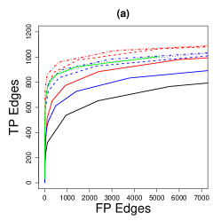
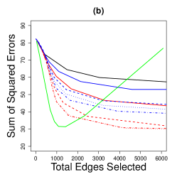
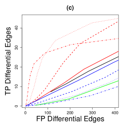
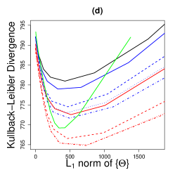
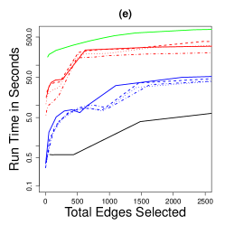
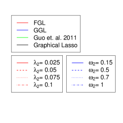
Figure 2: Performance of FGL, GGL, Guo et al. (2011)’s method, and the graphical lasso on simulated data with $150$ observations in each of 3 classes, and $500$ features. Black lines display models derived using the graphical lasso, green lines display the proposal of Guo et al. (2011), red lines display FGL, and blue lines display GGL. (a): The number of edges correctly identified to be nonzero (TP Edges) is plotted against the number of edges incorrectly identified to be nonzero (FP edges). (b): The sum of squared errors in edge values is plotted against the total number of edges estimated to be nonzero. (c): The number of edges correctly found to have values differing between classes (TP Differential Edges) is plotted against the number of edges incorrectly found to have values differing between classes (FP Differential Edges). (d): The dKL of the estimated models from the true models is plotted against the $\ell_{1}$ norm of the off-diagonal entries of the estimated precision matrices. (e): Running time (in seconds) is plotted against the number of non-zero edges estimated. Note the use of a log scale on the $y$-axis.

7.2 Performance as a function of $n$ and $p$

We now evaluate the effect of sample size $n$ and dimension $p$ on the performances of FGL and GGL.

7.2.1 Simulation set-up

We generate a pair of networks with $p=500$ much as described in Section 7.1.1, but with $K=2$ instead of $K=3$. The first network has 10 equal-sized components with power law degree distributions, and the second network is identical to the first in both edge identity and value, but with two components removed.

In addition to the 500-feature network pair, we generate a pair of networks with $p=1000$ features, each of which is block diagonal with $500\times 500$ blocks corresponding to two copies of the 500-feature networks just described. We generate covariance matrices from the networks exactly as described in Section 7.1.1.

7.2.2 Simulation results

For both the $p=500$ and the $p=1000$ networks, we simulate 100 datasets with $n=50$, $n=200$, and $n=500$ samples in each class. We run FGL with $\lambda_{1}=0.2,\lambda_{2}=0.1$ and GGL with $\lambda_{1}=0.05,\lambda_{2}=0.25$. We record in Table 1 dKL as well as the sensitivity and false discovery rate associated with detecting non-zero edges and detecting differential edges. In this simulation setting, accuracy of covariance estimation (as measured by dKL) improves significantly from $n=50$ to $n=200$, and improves only marginally with a further increase to $n=500$. Detection of edges improves throughout the range of $n$’s sampled: for both FGL and GGL, sensitivity improves slightly with increased sample size, and FDR decreases dramatically. Detection of edge differences is a more difficult problem, for which FGL performs well.

Table 1: Performances as a function of $n$ and $p$. Means over 100 replicates are shown for dKL, and for sensitivity (Sens.) and false discovery rate (FDR) of detection of edges (DE) and differential edge detection (DED).

$p$ $n$ dKL DE Sens. DE FDR DED Sens. DED FDR FGL 50 545.1 0.502 0.966 0.262 0.996 500 200 517.5 0.570 0.053 0.228 0.485 500 516.6 0.590 0.001 0.192 0.036 50 1119.3 0.600 0.970 0.245 0.998 1000 200 1035.0 0.666 0.063 0.223 0.557 500 1033.3 0.681 0.000 0.194 0.025 GGL 50 549.8 0.490 0.973 0.337 0.996 500 200 520.8 0.505 0.060 0.244 0.903 500 519.7 0.524 0.010 0.194 0.921 50 1127.9 0.587 0.976 0.316 0.998 1000 200 1041.7 0.615 0.061 0.239 0.908 500 1039.4 0.629 0.007 0.197 0.920

8 Analysis of lung cancer microarray data

We applied FGL to a dataset containing $22,283$ microarray-derived gene expression measurements from large airway epithelial cells sampled from 97 patients with lung cancer and 90 controls (Spira et al., 2007). The data are publicly available from the Gene Expression Omnibus (Barrett et al., 2005) at accession number GDS2771. We omitted genes with standard deviations in the bottom $20\%$ since a greater share of their variance is likely attributable to non-biological noise. The remaining genes were normalized to have mean zero and standard deviation one within each class. To avoid disparate levels of sparsity between the classes and to prevent the larger class from dominating the estimated networks, we weighted each class equally instead of by sample size in (2.4). Since our goal was data visualization and hypothesis generation, we chose a high value for the sparsity tuning parameter, $\lambda_{1}=0.95$, to yield very sparse network estimates. We ran FGL with a range of $\lambda_{2}$ values in order to identify the edges that differed most strongly, and settled on $\lambda_{2}=0.005$ as providing the most interpretable results. Application of Theorem 1 revealed that only 278 genes were connected to any other gene using the chosen tuning parameters. Identification of block diagonal structure using Theorem 1 and application of the FGL algorithm took less than two minutes. (Note that this data set is so large that it would be computationally prohibitive to apply the proposal of Guo et al. (2011)!) FGL estimated 134 edges shared between the two networks, 202 edges present only in the cancer network, and 18 edges present only in the normal tissue network. The results are displayed in Figure 3.

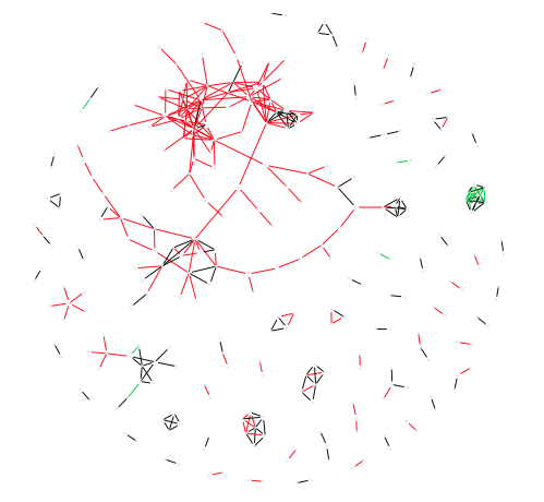
Figure 3: Conditional dependency networks inferred from 17,772 genes in normal and cancerous lung cells. 278 genes have nonzero edges in at least one of the two networks. Black lines denote edges common to both classes. Red and green lines denote tumor-specific and normal-specific edges, respectively.

The estimated networks contain many two-gene subnetworks common to both classes, a few small subnetworks, and one large subnetwork specific to tumor cells. Reassuringly, 45% of edges, including almost all of the two-gene subnetworks, connect multiple probes for the same gene. Many other edges connect genes that are obviously related, involved in the same biological process, or even coding for components of the same enzyme. Examples include TUBA1B and TUBA1C, PABPC1 and PABPC3, HLA-B and HLA-G, and SERPINB3 and SERPINB4. Recovery of these pairs suggests that FGL (and other network analysis tools) can generate high-quality hypotheses about gene co-regulation and functional interactions. This increases our confidence that some of the non-obvious two-gene subnetworks detected in this analysis may merit further investigation. Examples include DAZAP2 and TCP1, PRKAR1A and CALM3, and BCLAF1 and SERPB1. A complete list of subnetworks detected is available in the Supplementary Materials.

The small black and green network in Figure 3 suggests an interesting phenomenon. It contains multiple probes for two hemoglobin genes, HBA2 and HBB. In the normal tissue network, the probes for these genes are heavily interconnected both within and between the genes. In the tumor cells, while edges between HBA2 probes and between HBB probes are preserved, no edges connect the two genes. The abundance of connections between the two genes in healthy cells and the absence of connections in tumor cells may indicate a possible direction of future investigation.

The most promising results of this analysis arise from the large subnetwork (104 nodes for 84 unique genes) unique to tumor cells. Many of the subnetwork’s genes are involved in constructing ribosomes, including RPS8, RPS23, RPS24, RPS7p11, RPL3, RPL5, RPL10A, RPL14P1, RPL15, RPL17, RPL30 and RPL31. Other genes in the subnetwork further involve ribosome functioning: SRP14 and SRP9L1 are involved in recruiting proteins from ribosomes into the ER, and NACA inhibits the SRP pathway. Thus this subnetwork portrays a detailed web of relationships consistent with known biology. More interestingly, this network also contains two genes in the RAS oncogene family: RAB1A and RAB11A. Genes in this family have been linked to many types of cancer, and are considered promising targets for therapeutics (Adjei, 2008). These genes’ connections with ribosome activity in the tumor samples may indicate a relationship common to an important subset of cancers. Many other genes belong to this network, each indicating a potentially novel interaction in cancer biology.

9 Discussion

We have introduced the joint graphical lasso, a method for estimating sparse inverse covariance matrices on the basis of observations drawn from distinct but related classes. We employ an ADMM algorithm to solve the joint graphical lasso problem with any convex penalty function, and we provide explicit and efficient solutions for two useful penalty functions. Our algorithm is tractable on very large datasets ($>20,000$ features), and usually converges in seconds for smaller problems (500 features). Our joint estimation methods outperform competing approaches on a range of simulated datasets.

In the JGL optimization problem (2.4), the contribution of each class to the penalized log likelihood is weighted by its size; consequently, the largest class can have outsize influence on the estimated networks. By omitting the $n_{k}$ term in (2.4), it is possible to weight the classes equally to prevent a single class from dominating estimation.

We note that FGL and GGL’s reliance on two tuning parameters is a strength rather than a drawback: unlike the proposal of Guo et al. (2011), which involves a single tuning parameter that controls both sparsity and similarity, in performing FGL and GGL one can vary separately the amount of similarity and sparsity to enforce in the network estimates.

The joint graphical lasso has potential applications beyond those discussed in this paper. For instance, one could use it to shrink multiple classes’ precision matrices towards each other in order to define a classifier intermediate between quadratic discriminant analysis (QDA) and linear discriminant analysis (LDA) (Hastie et al., 2009). In fact, a similar approach has been taken in recent work (Simon & Tibshirani, 2012). In the unsupervised setting, it can be used in the maximization step of Gaussian model-based clustering in order to reduce the variance associated with estimating a separate covariance matrix for each cluster.

An R package implementing FGL and GGL will be made available on CRAN,
http://cran.r-project.org/.

Appendix 1: Modifying JGL to work on the scale of partial correlations

A reviewer suggested that under some circumstances, it may be preferable to encourage the $K$ networks to have shared partial correlations, rather than shared precision matrices. Below, we describe a simple approach for extending our FGL proposal to work on the scale of partial correlations. A similar approach can be taken to extend GGL. The extension relies on two insights.

1. $\rho_{ij}=-\frac{\sigma^{ij}}{\sqrt{\sigma^{ii}\sigma^{jj}}}$, where $\rho_{ij}$ is the true partial correlation between the $i$th and $j$th features, and where $\sigma^{ij}$ is the $(i,j)$th entry of the true precision matrix.

2. The algorithm for solving the FGL optimization problem can easily be modified to make use of the following penalty function:

   $$P(\{{\bf\Theta}\})=\sum_{k=1}^{K}\sum_{i\neq j}\lambda_{1,ij}|\theta^{(k)}_{ij}|+\sum_{k<k^{\prime}}\sum_{i,j}\lambda_{2,ij}|\theta^{(k)}_{ij}-\theta^{(k^{\prime})}_{ij}|,$$ (9.22)

where $\lambda_{t,ij}=\lambda_{t}/\sqrt{\hat{\sigma}^{ii}\hat{\sigma}^{jj}}$, $t=1,\ 2$, and where $\hat{\sigma}^{ii}$ is an estimate of the $i$th diagonal element of the $K$ precision matrices. (Here, we assume the $K$ precision matrices have shared diagonal elements.) The estimate $\{\hat{\sigma}^{ii}\}$ can be obtained in a number of ways, for instance by performing the graphical lasso on the samples from all $K$ data sets together. Then this approach will effectively result in applying a generalized fused lasso penalty to the partial correlations for the $K$ classes.

Appendix 2: Proofs of Theorems 1 and 2

Preliminaries to Proofs of Theorems 1 and 2

We begin with a few comments on subgradients. The subgradient of $|\theta_{ij}^{(k)}|$ with respect to $\theta_{ij}^{(k)}$ equals

$$\left\{\begin{array}[]{lll}1&\mbox{if $\theta_{ij}^{(k)}>0$}\\ -1&\mbox{if $\theta_{ij}^{(k)}<0$}\\ a&\mbox{if $\theta_{ij}^{(k)}=0$}\\ \end{array},\right.$$

for some $a\in[-1,1]$. The subgradient of $|\theta_{ij}^{(k)}-\theta_{ij}^{(k^{\prime})}|$ with respect to $(\theta_{ij}^{(k)},\theta_{ij}^{(k^{\prime})})$ for $k\neq k^{\prime}$ equals $(d,-d)$, where

$$d=\left\{\begin{array}[]{lll}1&\mbox{if $\theta_{ij}^{(k)}>\theta_{ij}^{(k^{\prime})}$}\\ -1&\mbox{if $\theta_{ij}^{(k)}<\theta_{ij}^{(k^{\prime})}$}\\ a&\mbox{if $\theta_{ij}^{(k)}=\theta_{ij}^{(k^{\prime})}$}\\ \end{array},\right.$$

for some $a\in[-1,1]$. Finally, the subgradient of $\sqrt{\sum_{k=1}^{K}(\theta_{ij}^{(k)})^{2}}$ with respect to $(\theta_{ij}^{(1)},\ldots,\theta_{ij}^{(K)})$ is given by

$$\left\{\begin{array}[]{ll}(\theta_{ij}^{(1)},\ldots,\theta_{ij}^{(K)})/\sum_{k=1}^{K}(\theta_{ij}^{(k)})^{2}&\mbox{if $\sum_{k=1}^{K}(\theta_{ij}^{(k)})^{2}>0$}\\ (\Upsilon_{1,ij},\ldots,\Upsilon_{K,ij})&\mbox{if $\theta_{ij}^{(1)}=\ldots=\theta_{ij}^{(K)}=0$}\\ \end{array},\right.$$

for some $\Upsilon_{1,ij},\ldots,\Upsilon_{K,ij}$ such that $\sum_{k=1}^{K}\Upsilon_{k,ij}^{2}\leq 1$.

To prove Theorem 1, we will use the following lemma.

Lemma 9.1.

The following two sets of conditions are equivalent:

• (A): $|n_{1}S_{1}|\leq\lambda_{1}+\lambda_{2}$, $|n_{2}S_{2}|\leq\lambda_{1}+\lambda_{2}$, and $|n_{1}S_{1}+n_{2}S_{2}|\leq 2\lambda_{1}$.

• (B): There exist $\Gamma_{1},\Gamma_{2},\Upsilon\in[-1,1]$ such that $-n_{1}S_{1}-\lambda_{1}\Gamma_{1}-\lambda_{2}\Upsilon=0$, and $-n_{2}S_{2}-\lambda_{1}\Gamma_{2}+\lambda_{2}\Upsilon=0$.

Proof.

We will begin by proving that $(B)$ implies $(A)$, and will then prove that $(A)$ implies $(B)$.

Proof that (B) $\Rightarrow$ (A):

First of all, $-n_{1}S_{1}-\lambda_{1}\Gamma_{1}-\lambda_{2}\Upsilon=0$ implies that $|n_{1}S_{1}|\leq\lambda_{1}+\lambda_{2}$, since $\Gamma_{1},\Upsilon\in[-1,1]$. Similarly, $-n_{2}S_{2}-\lambda_{1}\Gamma_{2}+\lambda_{2}\Upsilon=0$ implies that $|n_{2}S_{2}|\leq\lambda_{1}+\lambda_{2}$. Finally, summing the two equations in $(B)$ reveals that $n_{1}S_{1}+n_{2}S_{2}=-\lambda_{1}(\Gamma_{1}+\Gamma_{2})$, which implies that $|n_{1}S_{1}+n_{2}S_{2}|\leq 2\lambda_{1}$.

Proof that (A) $\Rightarrow$ (B):

Without loss of generality, assume that $n_{1}S_{1}\geq n_{2}S_{2}$. We split the proof into two cases.

1. Case 1: $n_{1}S_{1}-n_{2}S_{2}<2\lambda_{2}$.

   Let $\Gamma_{1}=\Gamma_{2}=\frac{-n_{1}S_{1}-n_{2}S_{2}}{2\lambda_{1}}$, and $\Upsilon=\frac{-n_{1}S_{1}+n_{2}S_{2}}{2\lambda_{2}}$.

   First, note that by (A), we know that $|n_{1}S_{1}+n_{2}S_{2}|\leq 2\lambda_{1}$. Therefore, $\Gamma_{1},\Gamma_{2}\in[-1,1]$. Second, note that Case 1’s assumption that $n_{1}S_{1}-n_{2}S_{2}<2\lambda_{2}$ implies that $\Upsilon\in[-1,1]$. Finally, we see by inspection that $-n_{1}S_{1}-\lambda_{1}\Gamma_{1}-\lambda_{2}\Upsilon=0$, and $-n_{2}S_{2}-\lambda_{1}\Gamma_{2}+\lambda_{2}\Upsilon=0$.

2. Case 2: $n_{1}S_{1}-n_{2}S_{2}\geq{2\lambda_{2}}$.

   Let $\Gamma_{1}=\frac{-n_{1}S_{1}+\lambda_{2}}{\lambda_{1}}$, $\Gamma_{2}=\frac{-n_{2}S_{2}-\lambda_{2}}{\lambda_{1}}$, and $\Upsilon=-1$. Then, by inspection, $-n_{1}S_{1}-\lambda_{1}\Gamma_{1}-\lambda_{2}\Upsilon=0$, and $-n_{2}S_{2}-\lambda_{1}\Gamma_{2}+\lambda_{2}\Upsilon=0$.

   It remains to show that $\Gamma_{1},\Gamma_{2},\Upsilon\in[-1,1]$. Trivially, $\Upsilon=-1\in[-1,1]$. From our assumption that $|n_{1}S_{1}|\leq\lambda_{1}+\lambda_{2}$, we know that $-1\leq\Gamma_{1}$. Moreover, by the assumptions that ${n_{1}S_{1}-n_{2}S_{2}}\geq{2\lambda_{2}}$ and $|n_{1}S_{1}+n_{2}S_{2}|\leq 2\lambda_{1}$, we have that

   $$\Gamma_{1}=\frac{-n_{1}S_{1}+\lambda_{2}}{\lambda_{1}}\leq\frac{-n_{1}S_{1}+\lambda_{2}\left(\frac{n_{1}S_{1}-n_{2}S_{2}}{2\lambda_{2}}\right)}{\lambda_{1}}=\frac{-n_{1}S_{1}-n_{2}S_{2}}{2\lambda_{1}}\leq 1.$$ (9.23)

   Therefore $\Gamma_{1}\in[-1,1]$.

   By the assumption that $|n_{2}S_{2}|\leq\lambda_{1}+\lambda_{2}$, we know that $\Gamma_{2}=\frac{-n_{2}S_{2}-\lambda_{2}}{\lambda_{1}}\leq 1$. From the assumptions that $n_{1}S_{1}-n_{2}S_{2}\geq 2\lambda_{2}$ and $|n_{1}S_{1}+n_{2}S_{2}|\leq 2\lambda_{1}$, we have that

   $$\Gamma_{2}=\frac{-n_{2}S_{2}-\lambda_{2}}{\lambda_{1}}\geq\frac{-n_{2}S_{2}-\lambda_{2}\left(\frac{n_{1}S_{1}-n_{2}S_{2}}{2\lambda_{2}}\right)}{\lambda_{1}}=\frac{-n_{1}S_{1}-n_{2}S_{2}}{2\lambda_{1}}\geq-1.$$ (9.24)

   Therefore $\Gamma_{2}\in[-1,1]$.

Thus we conclude (A) $\Rightarrow$ (B), and our proof of Lemma 9.1 is complete. ∎

We will make use of the following lemma in order to prove Theorem 2.

Lemma 9.2.

The following two conditions are equivalent:

• (A): There exist scalars $a_{1},\ldots,a_{K}$ such that $\sum_{k=1}^{K}a_{k}^{2}\leq 1$ and $n_{k}|S_{k}|\leq\lambda_{1}+\lambda_{2}a_{k}$ for all $k=1,\ldots,K$.

• (B): There exist scalars $\Gamma_{1},\ldots,\Gamma_{K}\in[-1,1]$ and $\Upsilon_{1},\ldots,\Upsilon_{K}$ such that $\sum_{k=1}^{K}\Upsilon_{k}^{2}\leq 1$ and $n_{k}S_{k}+\lambda_{1}\Gamma_{k}+\lambda_{2}\Upsilon_{k}=0$ for $k=1,\ldots,K$.

Proof.

We will begin by proving that $(B)$ implies $(A)$, and will then show that $(A)$ implies $(B)$.

Proof that ${(B)}\Rightarrow{(A)}$:

By $(B)$, $n_{k}|S_{k}|=|\lambda_{1}\Gamma_{k}+\lambda_{2}\Upsilon_{k}|\leq\lambda_{1}|\Gamma_{k}|+\lambda_{2}|\Upsilon_{k}|\leq\lambda_{1}+\lambda_{2}|\Upsilon_{k}|$. Letting $a_{k}=|\Upsilon_{k}|$, the result holds.

Proof that ${(A)}\Rightarrow{(B)}$:

Let $\Gamma_{k}$ and $\Upsilon_{k}$ take the following forms, for $k=1,\ldots,K$:

$$\Gamma_{k}=\begin{cases}-1&\mathrm{\;\;if\;\;}n_{k}S_{k}>\lambda_{1}\\ -n_{k}S_{k}/\lambda_{1}&\mathrm{\;\;if\;\;}-\lambda_{1}<n_{k}S_{k}<\lambda_{1}\\ 1&\mathrm{\;\;if\;\;}n_{k}S_{k}<-\lambda_{1}\end{cases}$$ (9.25)

$$\Upsilon_{k}=\begin{cases}(-n_{k}S_{k}+\lambda_{1})/\lambda_{2}&\mathrm{\;\;if\;\;}n_{k}S_{k}>\lambda_{1}\\ 0&\mathrm{\;\;if\;\;}-\lambda_{1}<n_{k}S_{k}<\lambda_{1}\\ (-n_{k}S_{k}-\lambda_{1})/\lambda_{2}&\mathrm{\;\;if\;\;}n_{k}S_{k}<-\lambda_{1}\end{cases}$$ (9.26)

First of all, we note by inspection that $\Gamma_{k}\in[-1,1]$ and that $n_{k}S_{k}+\lambda_{1}\Gamma_{k}+\lambda_{2}\Upsilon_{k}=0$ for $k=1,\ldots,K$. It remains to show that $\sum_{k=1}^{K}\Upsilon_{k}^{2}\leq 1$. Specifically, we will show that $\Upsilon_{k}^{2}\leq a_{k}^{2}$ for $k=1,\ldots,K$. To see why this is the case, note that if $-\lambda_{1}<n_{k}S_{k}<\lambda_{1}$ then $0=\Upsilon_{k}^{2}\leq a_{k}^{2}$. And if $n_{k}S_{k}>\lambda_{1}$ or $n_{k}S_{k}<-\lambda_{1}$, then $\Upsilon_{k}^{2}=\left(\frac{n_{k}|S_{k}|-\lambda_{1}}{\lambda_{2}}\right)^{2}\leq a_{k}^{2}$. ∎

Proof of Theorem 1

We first consider the claim for the case $K=2$. By the Karush-Kuhn-Tucker (KKT; see e.g. Boyd & Vandenberghe 2004) conditions, a necessary and sufficient set of conditions for $\{{\bf\Theta}\}$ to be the solution to the JGL problem is that

$$0 = n_{1}({\bf\Theta}^{(1)})^{-1}-n_{1}{\bf S}^{(1)}-\lambda_{1}{\bf\Gamma}_{1}-\lambda_{2}\bf\Upsilon$$

$$0 = n_{2}({\bf\Theta}^{(2)})^{-1}-n_{2}{\bf S}^{(2)}-\lambda_{1}{\bf\Gamma}_{2}+\lambda_{2}\bf\Upsilon,$$ (9.27)

where ${\Gamma}_{1,ij}$ is the subgradient of $|\theta_{ij}^{(1)}|$ with respect to $\theta_{ij}^{(1)}$, ${\Gamma}_{2,ij}$ is the subgradient of $|\theta_{ij}^{(2)}|$ with respect to $\theta_{ij}^{(2)}$, and $\Upsilon_{ij}$ is the subgradient of $|\theta_{ij}^{(1)}-\theta_{ij}^{(2)}|$ with respect to $\theta_{ij}^{(1)}$.

Let $C_{1}$ and $C_{2}$ be a partition of the $p$ variables into two nonoverlapping sets, with $C_{1}\cap C_{2}=\emptyset$, $C_{1}\cup C_{2}=\{1,\ldots,p\}$. Consider the matrices

$${\bf\Theta}^{(1)}=\left(\begin{array}[]{cc}{\bf\Theta}^{(1)}_{1}&0\\ 0&{\bf\Theta}^{(1)}_{2}\end{array}\right),\;\;{\bf\Theta}^{(2)}=\left(\begin{array}[]{cc}{\bf\Theta}^{(2)}_{1}&0\\ 0&{\bf\Theta}^{(2)}_{2}\end{array}\right),$$ (9.28)

where ${\bf\Theta}^{(1)}_{1}$ and ${\bf\Theta}^{(2)}_{1}$ solve the JGL problem on the features in $C_{1}$, and ${\bf\Theta}^{(1)}_{2}$ and ${\bf\Theta}^{(2)}_{2}$ solve the JGL problem on the features in $C_{2}$. By inspection of (9.27), ${\bf\Theta}^{(1)}$ and ${\bf\Theta}^{(2)}$ solve the entire JGL optimization problem if and only if for all $i\in C_{1}$, $j\in C_{2}$, there exist $\Gamma_{1,ij},\Gamma_{2,ij},\Upsilon_{ij}\in[-1,1]$ such that

$$-n_{1}S_{ij}^{(1)}-\lambda_{1}\Gamma_{1,ij}-\lambda_{2}\Upsilon_{ij} = 0$$

$$-n_{2}S_{ij}^{(2)}-\lambda_{1}\Gamma_{2,ij}+\lambda_{2}\Upsilon_{ij} = 0.$$ (9.29)

Therefore, by Lemma 9.1, the proof of the claim for the case $K=2$ is complete.

The derivation of the necessary condition for the case $K>2$ is simple and we omit it here.

Proof of Theorem 2

We note that Theorem 2’s condition (4.19) is equivalent to the following:

$$|n_{k}S^{(k)}_{ij}|\leq\lambda_{1}+\lambda_{2}a_{ij,k}\mathrm{\;\;for\;all\;\;}i\in C_{1},\;j\in C_{2},\;k=1,\ldots,K$$ (9.30)

where $a_{ij,1},\ldots,a_{ij,K}$ are scalars that satisfy $\sum_{k=1}^{K}a_{ij,k}^{2}\leq 1$. We will prove that (9.30) is necessary and sufficient for the variables in $C_{1}$ to be completely disconnected from those in $C_{2}$ in each of the resulting network estimates.

By the KKT conditions, a necessary and sufficient set of conditions for $\{{\bf\Theta}\}$ to be the solution to the JGL problem is that

$$0=n_{k}({\bf\Theta}^{(k)})^{-1}-n_{k}{\bf S}^{(k)}-\lambda_{1}{\bf\Gamma}_{k}-\lambda_{2}{\bf\Upsilon}_{k}$$ (9.31)

for $k=1,\ldots,K$. In (9.31), ${\Gamma}_{k,ij}$ is the subgradient of $|\theta_{ij}^{(k)}|$ with respect to $\theta_{ij}^{(k)}$, and $({\Upsilon}_{1,ij},\ldots,{\Upsilon}_{K,ij})$ is the subgradient of $\sqrt{\sum_{k=1}^{K}(\theta_{ij}^{(k)})^{2}}$ with respect to $(\theta_{ij}^{(1)},\ldots,\theta_{ij}^{(K)})$.

Let $C_{1}$ and $C_{2}$ be a partition of the $p$ variables into two nonoverlapping sets, with $C_{1}\cap C_{2}=\emptyset$, $C_{1}\cup C_{2}=\{1,\ldots,p\}$. Consider the matrices of the form

$${\bf\Theta}^{(k)}=\left(\begin{array}[]{cc}{\bf\Theta}^{(k)}_{1}&0\\ 0&{\bf\Theta}^{(k)}_{2}\end{array}\right)$$ (9.32)

for $k=1,\ldots,K$, where ${\bf\Theta}^{(1)}_{1},\ldots,{\bf\Theta}^{(K)}_{1}$ solve the JGL problem on the features in $C_{1}$, and ${\bf\Theta}^{(1)}_{2},\ldots,{\bf\Theta}^{(K)}_{2}$ solve the JGL problem on the features in $C_{2}$. By inspection of (9.31), ${\bf\Theta}^{(1)},\ldots,{\bf\Theta}^{(K)}$ solve the entire JGL optimization problem if and only if for all $i\in C_{1}$, $j\in C_{2}$, there exist $\Gamma_{1,ij},\ldots,\Gamma_{K,ij}\in[-1,1]$ and $\Upsilon_{1,ij},\ldots,\Upsilon_{K,ij}$ satisfying $\sum_{k=1}^{K}\Upsilon_{k,ij}^{2}\leq 1$ such that

$$-n_{k}S_{ij}^{(k)}-\lambda_{1}\Gamma_{k,ij}-\lambda_{2}\Upsilon_{k,ij}=0$$ (9.33)

Therefore, by Lemma 9.2, the proof is complete.

Appendix 3: Additional simulations for two-class datasets

We first present results for a simulation study similar to the one in Section 7.1, but with only two classes. Taking an approach similar to the one described in Section 7.1, we defined two networks with $p=500$ features belonging to ten equally sized unconnected subnetworks, each with a power law degree distribution. Of the ten subnetworks, eight have the same structure and edge values in both classes, and two are present in only one class. Class 1’s network has 490 edges, 94 of which are not present in class 2. We generated covariance matrices as described in Section 7.1.1. Again, we simulated 100 datasets with $n=150$ observations per class. The results shown in Figure 4 are similar to the results in Section 7.1.2.

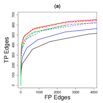
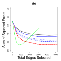
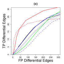
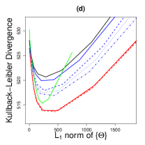
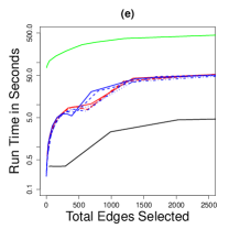
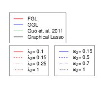
Figure 4: Performance of FGL, GGL, Guo et al. (2011)’s method, and the graphical lasso on simulated data with $150$ observations in each of 2 classes, and $500$ features corresponding to ten equally sized unconnected subnetworks drawn from a power law distribution. Details are as given in Figure 2.

We also simulated data with an entirely different network structure. Instead of the block-diagonal network structure used in the previous simulations, in this simulation we generated data drawn from a single large power law network. We defined class 1’s network to be a single power law network with only one component and generated ${\bf\Sigma}_{1}$ as described in Section 7.1.1. We then identified a branch in this network connected to the rest of the network through only one edge. We then let ${\bf\Sigma}_{2}^{-1}$ equal ${\bf\Sigma}_{1}^{-1}$, except for the elements corresponding to the edges in the selected branch, which were set to be zero instead. Finally, we defined ${\bf\Sigma}_{2}$ by inverting ${\bf\Sigma}_{2}^{-1}$, and generated the two classes’ data using ${\bf\Sigma}_{1}$ and ${\bf\Sigma}_{2}$. This yielded distributions based on two power law networks that were identical except for a missing branch in class 2. Class 1’s network has 499 edges, 104 of which are not present in class 2. We simulated 100 datasets with $n=150$ observations per class. Figure 5 shows the results, averaged over the 100 data sets. Again, FGL and GGL were superior to or competitive with the other methods.

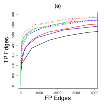
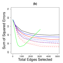
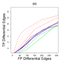
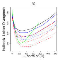
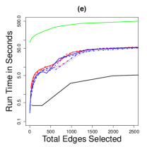
Figure 5: Performance of FGL, GGL, Guo et al. (2011)’s method, and the graphical lasso on simulated data with $150$ observations in each of 2 classes, and $500$ features corresponding to a single large power law network. Details are as given in Figure 2.

Appendix 4: Network structure used in simulations

The network structure for the simulations described in Section 7.1 is displayed in Figure 6. Black edges are shared between all three classes’ networks, green edges are present only in classes 1 and 2, and red edges are present only in class 1.

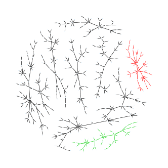
Figure 6: Network used to generate simulated datasets for Figure 2 in Section 7.1.2. Black edges are common to all three classes, green edges are present only in classes 1 and 2, and red edges are present only in class 1.

References

- (1)
- Adjei (2008) Adjei, A. (2008), ‘K-ras as a target for lung cancer therapy’, Journal of Thoractic Oncology 3(6), S160–S163.
- Ahmed & Xing (2009) Ahmed, A. & Xing, E. (2009), ‘Tesla: Recovering time-varying networks of dependencies in social and biological studies’, Proc. Natl. Acad. Sci. 29, 11878–11883.
- Barrett et al. (2005) Barrett, T., Suzek, T., Troup, D., Wilhite, S., Ngau, W., Ledoux, P., Rudnev, D., Lash, A., Fujibuchi, W. & Edgar, R. (2005), ‘NCBI GEO: mining millions of expression profiles–database and tools’, Nucleic Acids Research 33, D562–D566.
- Boyd et al. (2010) Boyd, S., Parikh, N., Chu, E., Peleato, B. & Eckstein, J. (2010), ‘Distributed optimization and statistical learning via the alternating direction method of multipliers’, Foundations and Trends in Machine Learning 3(1), 1–122.
- Boyd & Vandenberghe (2004) Boyd, S. & Vandenberghe, L. (2004), Convex Optimization, Cambridge University Press.
- Chen & Sharp (2004) Chen, H. & Sharp, B. (2004), ‘Content-rich biological network constructed by mining pubmed abstracts’, BMC Bioinformatics 5:147.
- Friedman, Hastie, Hoefling & Tibshirani (2007) Friedman, J., Hastie, T., Hoefling, H. & Tibshirani, R. (2007), ‘Pathwise coordinate optimization’, Annals of Applied Statistics 1, 302–332.
- Friedman, Hastie & Tibshirani (2007) Friedman, J., Hastie, T. & Tibshirani, R. (2007), ‘Sparse inverse covariance estimation with the graphical lasso’, Biostatistics 9, 432–441.
- Friedman et al. (2010) Friedman, J., Hastie, T. & Tibshirani, R. (2010), ‘A note on the group lasso and a sparse group lasso’, Technical report, Department of Statistics, Stanford University .
- Guo et al. (2011) Guo, J., Levina, E., Michailidis, G. & Zhu, J. (2011), ‘Joint estimation of multiple graphical models’, Biometrika 98(1), 1–15.
- Hastie et al. (2009) Hastie, T., Tibshirani, R. & Friedman, J. (2009), The Elements of Statistical Learning; Data Mining, Inference and Prediction, Springer Verlag, New York.
- Hocking et al. (2011) Hocking, L., Joulin, A. & Bach, F. (2011), ‘Clusterpath: An algorithm for clustering using convex fusion penalties’, Proceedings of the 28th International Conference on Machine Learning .
- Hoefling (2010a) Hoefling, H. (2010a), personal communication.
- Hoefling (2010b) Hoefling, H. (2010b), ‘A path algorithm for the fused lasso signal approximator’, Journal of Computational and Graphical Statistics 19(4), 984–1006.
- Kolar et al. (2010) Kolar, M., Song, L., Ahmed, A. & Xing, E. (2010), ‘Estimating time-varying networks’, Annals of Applied Statistics 4 (1), 94–123.
- Kolar & Xing (2009) Kolar, M. & Xing, E. (2009), ‘Sparsistent estimation of time-varying discrete markov random fields’, Manuscript, arXiv:0907.2337 .
- Lauritzen (1996) Lauritzen, S. (1996), Graphical Models, Oxford Science Publications.
- Li et al. (2011) Li, S., Hsu, L., Peng, J. & Wang, P. (2011), ‘Bootstrap inference for network construction’, Manuscript, arXiv:1111.5028v1 .
- Mazumder & Hastie (2012) Mazumder, R. & Hastie, T. (2012), ‘Exact covariance-thresholding into connected components for large-scale graphical lasso’, Journal of Machine Learning Research 13, 723–736.
- Meinshausen & Buhlmann (2010) Meinshausen, M. & Buhlmann, P. (2010), ‘Stability selection (with discussion)’, Journal of the Royal Statistical Society, Series B 72, 417–473.
- Meinshausen (2007) Meinshausen, N. (2007), ‘Relaxed lasso’, Computational Statistics and Data Analysis 52, 374–393.
- Meinshausen & Bühlmann (2006) Meinshausen, N. & Bühlmann, P. (2006), ‘High dimensional graphs and variable selection with the lasso’, Annals of Statistics 34, 1436–1462.
- Mohan et al. (2012) Mohan, K., Chung, M., Han, S., Fazel, M., Witten, D. & Lee, S. (2012), ‘Structured sparse learning of multiple Gaussian graphical models’.
- Peng et al. (2009) Peng, J., Wang, P., Zhou, N. & Zhu, J. (2009), ‘Partial correlation estimation by joint sparse regression model’, Journal of the American Statistical Association 104(486), 735–746.
- Rothman et al. (2008) Rothman, A., Levina, E. & Zhu, J. (2008), ‘Sparse permutation invariant covariance estimation’, Electronic Journal of Statistics 2, 494–515.
- Simon & Tibshirani (2012) Simon, N. & Tibshirani, R. (2012), ‘Discriminant analysis with adaptively pooled covariance’, Manuscript, arXiv:1111.1687 .
- Song et al. (2009a) Song, L., Kolar, M. & Xing, E. (2009a), ‘Keller: Estimating time-evolving interactions between genes’, Bioinformatics 25 (12), i128–i136.
- Song et al. (2009b) Song, L., Kolar, M. & Xing, E. (2009b), ‘Time-varying dynamic bayesian networks’, Proceeding of the 23rd Neural Information Processing Systems .
- Spira et al. (2007) Spira, A., Beane, J., Shah, V., Steiling, K., Liu, G., Schembri, F., Gilman, S., Dumas, Y., Calner, P., Sebastiani, P., Sridhar, S., Beamis, J., Lamb, C., Anderson, T., Gerry, N., Keane, J., Lenburg, M. & Brody, J. (2007), ‘Airway epithelial gene expression in the diagnostic evaluation of smokers with suspect lung cancer’, Nature Medicine 13(3), 361–366.
- Tarjan (1972) Tarjan, R. (1972), ‘Depth-first search and linear graph algorithms’, SIAM Journal on Computing 1(2), 146–160.
- Tibshirani (1996) Tibshirani, R. (1996), ‘Regression shrinkage and selection via the lasso’, J. Royal. Statist. Soc. B. 58, 267–288.
- Tibshirani (2012) Tibshirani, R. (2012), personal communication.
- Tibshirani et al. (2005) Tibshirani, R., Saunders, M., Rosset, S., Zhu, J. & Knight, K. (2005), ‘Sparsity and smoothness via the fused lasso’, J. Royal. Statist. Soc. B. 67, 91–108.
- Witten et al. (2011) Witten, D., Friedman, J. & Simon, N. (2011), ‘New insights and faster computations for the graphical lasso’, Journal of Computational and Graphical Statistics 20(4), 892–900.
- Witten & Tibshirani (2009) Witten, D. & Tibshirani, R. (2009), ‘Covariance-regularized regression and classification for high-dimensional problems’, J. Royal. Stat. Soc. B. 71(3), 615–636, PMCID:PMC2806603.
- Yuan & Lin (2007a) Yuan, M. & Lin, Y. (2007a), ‘Model selection and estimation in regression with grouped variables’, Journal of the Royal Statistical Society, Series B 68, 49–67.
- Yuan & Lin (2007b) Yuan, M. & Lin, Y. (2007b), ‘Model selection and estimation in the Gaussian graphical model’, Biometrika 94(10, 19–35.
- Zhou et al. (2008) Zhou, S., Lafferty, J. & Wasserman, L. (2008), ‘Time varying undirected graphs’, The 21st Annual Conference on Learning Theory (COLT 2008), Helsinki, Finland .