Pulsar Emission Geometry and Accelerating Field Strength

Abstract

The high-quality Fermi LAT observations of gamma-ray pulsars have opened a new window to understanding the generation mechanisms of high-energy emission from these systems. The high statistics allow for careful modeling of the light curve features as well as for phase resolved spectral modeling. We modeled the LAT light curves of the Vela and CTA 1 pulsars with simulated high-energy light curves generated from geometrical representations of the outer gap and slot gap emission models, within the vacuum retarded dipole and force-free fields. A Markov Chain Monte Carlo maximum likelihood method was used to explore the phase space of the magnetic inclination angle, viewing angle, maximum emission radius, and gap width. We also used the measured spectral cutoff energies to estimate the accelerating parallel electric field dependence on radius, under the assumptions that the high-energy emission is dominated by curvature radiation and the geometry (radius of emission and minimum radius of curvature of the magnetic field lines) is determined by the best fitting light curves for each model. We find that light curves from the vacuum field more closely match the observed light curves and multiwavelength constraints, and that the calculated parallel electric field can place additional constraints on the emission geometry.

I INTRODUCTION

The pulsar emission mechanism is not well understood. Magnetospheric particle acceleration is likely responsible for the observed emission, but the emission geometry is unknown. One can gain some insight by comparing light curves derived from geometrical emission models with observed pulsar light curves. Observations of pulsars by the Fermi Gamma-ray Space Telescope Large Area Telescope (LAT) Atwood2009 have shown that the high-energy emission likely originates in the outer magnetosphere PSRCat . We simulated high-energy light curves from geometrical versions of two standard high-altitude emission models, the outer gap (OG) Romani_OG and slot gap (SG) Muslimov_SG , and from a third, modified SG model with azimuthal asymmetry in emissivity due to a naturally occurring offset dipole (aSG) Harding_aSG . These models were considered within two field geometries, the vacuum retarded dipole (VRD) and force-free (FF) Contopoulos_FF fields. We compared the resulting light curves with the LAT light curves of the Vela pulsar and PSR J0007+7303, the CTA 1 pulsar, to constrain the systems’ geometries, and calculated the model-dependent magnitude of the accelerating electric field $E_{||}$ in the VRD field.

II LIGHT CURVE MODELING

To model the LAT light curves, we first simulated pulsar light curves from geometrical representations of the SG, aSG, and OG emission zones within the VRD and FF fields, following the simulation method of Dyks2004 . The $B$ field defined in the observer’s frame is transformed to the co-rotating frame (CF) Bai_FF and photons are emitted tangent to B in the CF prior to calculation of the aberration. We assume constant emissivity along the field lines in the CF. The azimuthal asymmetry in the polar cap (PC) angle for the aSG model is calculated for each inclination angle $\alpha$ as in Harding_aSG (see also Harding_theseproc ). For a given $\alpha$, gap width $w$ (in units of open volume coordinates $r_{\mathrm{ovc}}$, as in Dyks2004 ), and maximum emission altitude $r$, the code outputs the dimensionless emission intensity and the minimum and maximum radii of curvature, $\rho_{\mathrm{min}}$ and $\rho_{\mathrm{max}}$, emission radii $r_{\mathrm{min}}$ and $r_{\mathrm{max}}$, and local field magnitude $|B|_{\mathrm{min}}$ and $|B|_{\mathrm{max}}$, at all observer angles $\zeta$ and rotation phases $\phi$.

We simulated light curves for a fiducial rotation period of 0.1 s on a 4-dimensional grid of $\alpha$, $\zeta$, $w$, and $r$. Our simulation resolutions are $1^{\circ}$ in $\alpha$ for the VRD field and $15^{\circ}$ for the FF magnetosphere; $1^{\circ}$ in $\zeta$; $0.01\,r_{\mathrm{ovc}}$ in $0\,r_{\mathrm{ovc}}\leq w\leq 0.3\,r_{\mathrm{ovc}}$; and $0.1\,R_{\mathrm{lc}}$ in $0.7\,R_{\mathrm{lc}}\leq r\leq 2.0\,R_{\mathrm{lc}}$, where $R_{\mathrm{lc}}=c/\Omega$ is the light cylinder radius. Emission is allowed out to a cylindrical radius $r_{\mathrm{cyl}}=0.98\,R_{\mathrm{lc}}$ for the OG model and $r_{\mathrm{cyl}}=0.95\,R_{\mathrm{lc}}$ for the SG models.

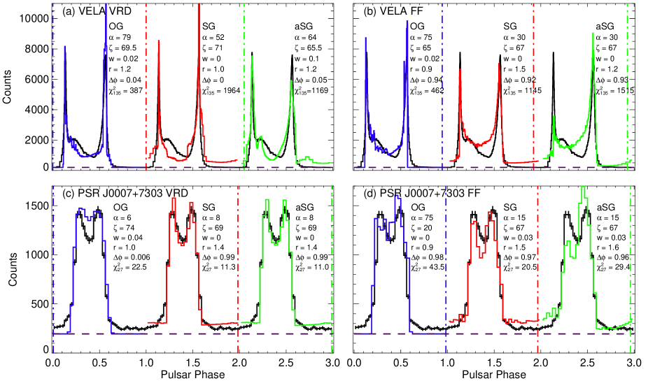
Figure 1: Light curve modeling results for Vela and PSR J0007+7303. The absolute best fit parameters are given next to each model; uncertainties in individual parameters vary, but are typically of order $\sim 10$%. In all panels, the light curve is shown in black. Blue curves show the best fit OG light curve, red the best fit SG light curve, and green the best aSG light curve. Vertical dot-dashed lines show phase zero of the model light curve of corresponding color; the phase of the line is the same as the listed $\Delta\phi$, and is the phase of emission coming from the closest magnetic pole. The horizontal purple dashed lines show the background count level. Panel (a) shows results for the Vela pulsar with the VRD field, (b) Vela with the FF field, (c) PSR J0007+7303 with the VRD field, and (d) PSR J0007+7303 with the FF field.

LAT light curves were constructed from photons in an angular radius $\theta<\mathrm{max}[1.6-3\mathrm{log}_{10}(E),1.3]$ from the pulsar Vela_2 . The PSR J0007+7303 light curve has 32 fixed-width bins, and was taken from CTA1_2 . The Vela light curve has 140 fixed-count bins of $\sim 3000$ photons each. The background of PSR J0007+7303, 195 counts/bin, was found using the Fermi tool gtsrcprob as in CTA1_2 . The emission in the off-peak above the background level was assumed to be magnetospheric in origin (but see CTA1_2 for details). The Vela background was found to be 204 counts/bin using the off-peak (phases 0.8-1, where no magnetospheric emission was detected in our spectral fits) counts in the energy-dependent PSF of the pulsar.

We used a Markov Chain Monte Carlo (MCMC) maximum likelihood routine Verde2003 to search the parameter space for the combination of ($\alpha$, $\zeta$, $w$, $r$, $\Delta\phi$) that best reproduced the LAT light curves. The fifth parameter, $\Delta\phi$, is the amount by which a model light curve must shift in phase in order to best match the LAT light curve. The MCMC begins at a random point in parameter space, calculates the likelihood $L$, and moves in a random direction to a new point in space to calculate $L$ again. If $L/L_{\mathrm{former}}>1$ or $>\mathrm{rand}[0,1)$, $L$ is saved in a chain; the routine runs until the chain contains the user-specified number of steps. Many chains were run to explore the whole parameter space. We used Wilks’ theorem, $\Delta\,$ln$\,L=-\Delta\chi^{2}/2$, to calculate $L$ at each point in parameter space. To perform a fit, we subtracted the background level from the LAT light curve, re-binned the model to match the data, and normalized the model to the total counts in the LAT light curve. For each fit in the vacuum case, we ran 200 chains with 20 steps each to adequately sample the parameter space. For the FF fits, we ran 20 chains of 20 steps each for each $\alpha$. Multi-wavelength constraints on $\alpha$ and $\zeta$ were considered after fitting. Our fit results are shown in Figure 1. Each plot shows three instances of the LAT light curve with the best OG, SG, and aSG light curve superposed. The zero phases of each model, corresponding to the nearest magnetic pole, are given by the vertical lines, and the background levels with horizontal lines.

We find that for the (a) VRD and (b) FF fields, the OG model (blue) statistically fits the Vela light curve better than either SG model. The SG (red) produces too much off-peak emission, leading to high $\chi^{2}$ values. The aSG (green) reduces the background significantly, leading to a much better fit. The aSG also qualitatively fits the peak emission well, as its main peaks are the correct approximate height and an inner peak is present. All three fits have $\zeta$ close to the value determined from the X-ray torus geometry [10], $\zeta\sim 64^{\circ}$. $\Delta\phi$ is consistent with the observed phase lag between the radio and $\gamma$-ray peaks for the VRD models; however, for the FF case, $\Delta\phi$ is too large.

For the pulsar in CTA 1, the SG models fit much better than the OG in both field geometries. There is no constraint on $\Delta\phi$ due to the lack of a radio detection. The VRD geometry in (c) produces much better fits than the FF in (d); there is little difference between the SG and aSG due to the small $\alpha$. A larger FF $\alpha$ leads to a larger PC offset, which lowers the first peak. The large difference between $\alpha$ and $\zeta$ is consistent with the pulsar being radio-quiet due to geometry–the radio beam would not cross our line of sight for such a large $|\alpha-\zeta|$.

III CALCULATION OF $E_{||}$

The $\gamma$-ray spectra of pulsars are well fit by an exponentially cut-off power law,

$$\frac{dN}{dE}=N_{0}\left(\frac{E}{E_{0}}\right)^{-\Gamma}\exp{\left[-\left(\frac{E}{E_{\mathrm{c}}}\right)^{b}\right]}\,\mathrm{ph}\,\,\mathrm{cm}^{-2}\,\mathrm{s}^{-1}\,\mathrm{MeV}^{-1}$$ (1)

where $N_{0}$ is the differential flux, $E_{0}$ the energy scale, $\Gamma$ the power law index, and $E_{\mathrm{c}}$ the cutoff energy; $b=1$ results in a simple exponential cutoff, while $b<1$ gives a sub-exponential cutoff and $b>1$ a super-exponential cutoff. For phase averaged spectra, $b<1$ due to blending of $E_{\mathrm{c}}$ as it varies with phase (e.g. Vela_2 ), while $b$ is consistent with (and is fixed to) 1 in individual phase bins.

In current models of pulsar emission, at energies above $\sim 100\,$MeV the emission is dominated by curvature radiation. Particles reach the radiation reaction limit at Lorentz factors $\gamma_{\mathrm{CR}}\sim 10^{7}$. In this limit, the curvature radiation cutoff energy $E_{\mathrm{CR}}$ is related to $E_{||}$ and $\rho_{\mathrm{c}}$ by

$$E_{\mathrm{CR}}=\frac{3}{2}\frac{\lambdabar}{\rho_{\mathrm{c}}}\gamma^{3}_{\mathrm{CR}}=0.32\lambda_{\mathrm{c}}\left(\frac{E_{||}}{e}\right)^{3/4}\rho_{\mathrm{c}}^{1/2}$$ (2)

Assuming all emission with $E>100\,$MeV is due to pure curvature radiation and that the VRD is the true $B$ field structure, we calculated $E_{||}$ in each light curve phase bin. We used the simulated minimum radii of curvature ($\rho_{\mathrm{c}}=\rho_{\mathrm{min}}$) from the best fit VRD light curves of §3 and the measured cutoff energies ($E_{\mathrm{CR}}=E_{\mathrm{c}}$) in each phase bin. The cutoff energies are given in CTA1_2 for PSR J0007+7303. We updated the Vela 0.1–100 GeV phase resolved spectral results with 30 months of LAT data, following the method of Vela_2 with 3000 pulsed counts per bin, and used our measured cutoff energies for the Vela $E_{||}$ calculation. As an example, Figure 2 shows the measured $E_{\mathrm{c}}$, the simulated $\rho_{\mathrm{min}}$, $r_{\mathrm{min}}$, and $|B|_{\mathrm{max}}$, and the calculated $E_{||}$ for the Vela pulsar peak emission (phases $0\leq\phi\leq 0.8$), using the best fit parameters from the VRD SG geometry.

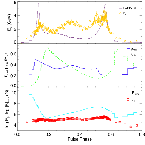
Figure 2: Example of simulated and measured values described in §3. (a) The LAT light curve of Vela (purple) and measured $E_{\mathrm{c}}$ with phase (yellow diamonds). (b) Simulated $\rho_{\mathrm{min}}$ (solid blue) and $r_{\mathrm{min}}$ (dashed green) for the best VRD SG fit parameters. (c) Simulated $|B|_{\mathrm{max}}$ (solid cyan) and calculated $E_{||}$ (red squares) for the best VRD SG fit parameters.

We explore how the parallel electric field varies with emission altitude. We have calculated $E_{||}$ in each phase bin for the best fit vacuum OG and SG model parameters. Because the value of $|B|_{\mathrm{max}}$ corresponds to $r_{\mathrm{min}}$, we have plotted $E_{||}$ and $E_{||}/|B|_{\mathrm{max}}$ with minimum emission radius for the OG and SG models in Figure 3.

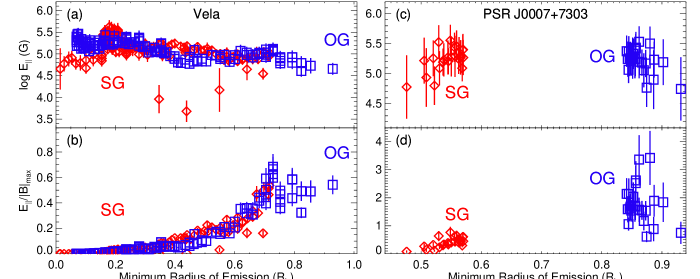
Figure 3: $E_{||}$ (a) and the ratio of $E_{||}/|B|_{\mathrm{max}}$ (b) for the OG (blue squares) and SG (red diamonds) models that best fit the Vela LAT light curve. (c) Same as (a) for PSR J0007+7303. (d) Same as (b) for PSR J0007+7303.

For both emission models, Vela has overall a $\sim\,$constant or gradually varying $E_{||}$ with altitude (panel $(a)$ of Figure 3), which is expected (e.g. Vela_2 ). In panel $(b)$, the value of $E_{||}$ is compared with $|B|_{\mathrm{max}}$. As expected for an $E$ field induced by $B$, the ratio $E_{||}/|B|_{\mathrm{max}}<1$ for all $r_{\mathrm{min}}$ out to the light cylinder radius (near and beyond $1\,R_{\mathrm{lc}}$, the vector components of B are less certain and are not included in this calculation).

For PSR J0007+7303, the magnitude of $E_{||}$ with $r_{\mathrm{min}}$ is consistent with a constant (panel $(c)$), and its values are similar to those calculated for Vela. Note that the geometrical parameters obtained from the light curve fits are very different from those of Vela, leading to a different range of $r_{\mathrm{min}}$ for PSR J0007+7303. The ratio $E_{||}/|B|_{\mathrm{max}}<1$ for the best fit SG model, but it is $>1$ for the best fit parameters of the OG model. There are instances in, for example, a non-ideal magnetosphere Kalapotharakos2011 where $E_{||}$ may be $>|B|$. In the case of the vacuum field, in which there are no currents, the only source of $E_{||}$ is induction by $B$, and therefore $E_{||}$ cannot be larger than $|B|_{\mathrm{max}}$. In this particular case, then, we find that the combination of the OG model and VRD field we have used does not approximate the physical environment of the pulsar magnetosphere and/or the geometry of the emission zone.

IV CONCLUSIONS

We have evaluated the geometries of the slot gap and outer gap emission models, and the vacuum retarded dipole and force-free magnetic field solutions, by comparing the simulated light curves with the LAT light curves of Vela and PSR J0007+7303 and finding the geometrical model parameters that best reproduce the data in each case. In general, the OG has no off-peak emission (this is largely responsible for the OG fitting Vela the best and PSR J0007+7303 the worst), while the SG models do a better job of reproducing wing emission but over-predict the off-peak emission. Introducing azimuthal asymmetry of the PC angle in the aSG model leads to a reduction in the off-peak emission level, improving upon the SG model light curve fits within the VRD field. In the FF field, however, aSG light curves tend to have a much reduced first peak, leading to significantly worse light curve fits.

The first $\gamma$-ray peak occurs at later phase in FF light curves, so values of $\Delta\phi$ are larger in the FF magnetosphere than in the VRD field. Physically, $\Delta\phi$ cannot be larger than the phase lag between the radio and first $\gamma$-ray peak unless the radio beam model is highly contrived. The FF field requires a $\Delta\phi$ larger than this phase lag for Vela. This suggests that the true pulsar magnetosphere may be significantly different from the FF magnetosphere.

For Vela, all fits within the VRD field have $\zeta$ close to the expected value of $64^{\circ}$, and all have reasonable values of $|\alpha-\zeta|$ such that the radio emission is observable. Interestingly, the aSG model has $\zeta$ closest to $64^{\circ}$, and while its $\chi^{2}$ is poor, it is an improvement over the SG and qualitatively reproduces well the major features (two main peaks and inner peak) of the pulsed emission. The FF fits also get close to the correct $\zeta$ value, but only the OG has an acceptable $|\alpha-\zeta|$, while the best fit SG models are consistent with a radio-quiet pulsar. Both field structures lead to large $|\alpha-\zeta|$ for PSR J0007+7303, consistent with the lack of detected radio emission.

We calculated the model-dependent $E_{||}$ for the OG and SG geometries, and found that it is constant or slowly varying with emission radius. Comparing $E_{||}$ with $|B|_{\mathrm{max}}$ leads to the interesting result that for PSR J0007+7303, $E_{||}>|B|_{\mathrm{max}}$ for the OG parameters that best fit the LAT light curve. This is not consistent with the VRD where $|E|<|B|$, and thus disfavors the OG model in the VRD geometry at the location in parameter space where the best light curve fit is found. The calculation of $E_{||}$ can therefore be used as a diagnostic of the model magnetosphere and emission geometry, in addition to the light curve fitting.

We cannot rule in favor of the SG or OG from these light curve fits. As the models are purely geometrical, we expect to reproduce only dominant light curve features, and our statistical fits are poor. The vacuum field produces better light curve fits than the force-free field. However, we note that the resolution in $\alpha$ of our FF models is much lower than in the VRD, so further modeling with higher resolution is needed to confirm this result. We have demonstrated that light curve modeling leads to constraints on the geometry of individual systems, and that the phase lag is an important diagnostic in comparing magnetic field structures. The model-dependent calculation of $E_{||}$, and comparison with the model $|B|_{\mathrm{max}}$, can additionally be used to constrain both the magnetosphere and emission geometry.

- (1) Abdo et al. 2010, ApJS 187, 460.
- (2) Abdo et al. 2010, ApJ 713, 154.
- (3) Abdo et al. 2011 (arXiv:1107.4151)
- (4) Atwood et al. 2009, ApJ 697, 1071.
- (5) Bai & Spitkovsky 2010, ApJ 715, 1282.
- (6) Contopoulos & Kalapotharakos 2010, MNRAS 404, 767.
- (7) Dyks et al. 2004, ApJ 614, 869.
- (8) Harding & Muslimov 2011, ApJ 726, 10.
- (9) Harding et al. 2011, these proceedings.
- (10) Kalapotharakos et al. 2011 (arXiv:1108.2138)
- (11) Muslimov & Harding 2004, ApJ 606, 1143.
- (12) Ng & Romani 2008, ApJ 673, 411.
- (13) Romani & Yadigaroglu 1995, ApJ 438, 314.
- (14) Verde et al. 2003, ApJS 148, 195.