Magnetic field of young star RW Aur

PACS numbers: 97.10.Bt; 97.10.Ld; 97.10.Gz; 97.10.Me

Key words: Stars – individual: RW Aur, T Tau – T Tauri stars – magnetic field – accretion – wind

Abstract

Results of longitudinal magnetic field $B_{z}$ measurements for young star RW Aur A are presented. We found that $B_{z}$ in the formation region of He I 5876 line’s narrow component varies from $-1.47\pm 0.15$ kG to $+1.10\pm 0.15$ kG. Our data are consistent with a stellar rotational period of $\simeq 5.6^{d}$ and with a model of two hotspots with an opposite polarity of magnetic field and with a difference in a longitude about $180^{o}.$ The spot with $B_{z}<0$ is located at the hemisphere above the midplane of RW Aur’s accretion disc and the spot with $B_{z}>0$ is below the midplane.

The following upper limits for $B_{z}$ (at $3\sigma$ level) were found after averaging of all our observations: 180 G for photosperic lines, 220 G and 230 G for formation regions of H_α and [OI] 6300 lines respectively. Upper limit 600 G were found in the region where broad components of emisson lines form.

For two cases out of 11 we observed the field in a formation region of a blue absorption wing of Na I D lines i.e. in an outflow: $B_{z}=-180\pm 50$ G and $-810\pm 80$ G.

Radial velocity of RW Aur’s photospheric lines averaged over all our observations is $\simeq+10.5$ km s^-1 what is 5.5 km s^-1 less than value derived ten years earlier by Petrov et al. (2001). In this connection, we discuss a possibility that RW Aur is not a binary but a triple system.

Introduction

T Tauri Stars are young $(t<10^{7}$ yr) low mass $(M\leq 2\,M_{\odot})$ stars at a stage of a gravitational contraction towards the main sequence. Magnetic fields determine an activity of TTS and play a crucial role in an evolution of angular momentum of these objects, therefore a question about strength and topology of the magnetic field is one of the fundamental questions of physics of young stars. Magnetic field was found in $\sim 10$ TTSs at the moment, and for some of them an information about its structure has been retrieved – see Donati & Landstreet (2009) and references therein.

RW Aur was included in the original list of T Tauri stars compiled by Joy (1945). The year before Joy and van Biesbroeck (1944) have discovered that the star (RW Aur A) has a companion (RW Aur B) at the distance $\simeq 1.2^{\prime\prime}$. It was found later that both components are so-called classical T Tauri stars (CTTS), whose activity is due to accretion of matter from protoplanetary disc (Bertout, 1989). Recently images of the discs were obtained for both components of the system in the submillimeter region (Cabrit et al., 2006). Contribution of the secondary to the overall optical flux does not exceed a few percent (Petrov et al., 2001), therefore it can be assumed that features of optical spectra described below belong to the primary.

Optical spectra of RW Aur were investigated by many researches – see Petrov et al. (2001); Alencar et al. (2005); Petrov & Kozack (2007) and references therein. It was found that the spectrum has a multicomponent structure which includes:

1) a photospheric absorption K1-K4 spectrum superimposed with emission continuum and narrow absorption lines with radial velocities close to that of photospheric lines;

2) absorption components in red wings of some lines that indicate gas inflow onto the star with velocity up to 400 km s^-1;

3) absorption components at blue wings of some lines, which indicate a gas outflow from stellar vicinity with a velocity greater than 200 km s^-1. The outflowing gas is collimated into two jets with an opposite orientation at large distances from the star (Hirth et al. 1994). Lines of [O I] and [S II] are originated in these jets;

4) emission lines of different elements which are (in a differnt degree) superposition of a broad (FWHM$\sim 100-200$ km s^-1) and narrow (FWHM $\sim 50$ km s^-1) components. The components are most likely formed in different regions.

Petrov et al. (2001) have found periodic variations of radial velocities of photospheric lines with an amplitude about 6 km s^-1 and a period $\simeq 2.77$ days. The same period was found for variations of radial velocity $V_{r}^{NC}$ an equivalent width $EW_{NC}$ of narrow emission component of He I 5876 line as well as an equivalent width EW_RA of an absorption feature in line’s red wing. Velocities $V_{r}^{ph}$ and $V_{r}^{NC}$ vary in antiphase and phase curves of $EW_{NC}$ and $EW_{RA}$ are shifted relative to the curve $V_{r}^{ph}$ to one fourth of the period. Similar behaviour of the narrow components and absorptions at the red wing is also observed for some other lines. What about broad components of emission lines it turned out that they vary with a period of about 5.5 days, i.e. twice slower than $V_{r}^{ph}.$

These features of RW Aur spectrum can be explained by a model of non-axisymmetric magnetospheric accretion. Petrov et al. (2001) have considered two possible reasons for a violation of an axisymmetry. The first reason is an existence of low-mass companion with an orbital period of 2.77 days. It was assumed that an interaction of the companion and the disc results in a fall of disc matter towards RW Aur A in a form of stream, which rotates together with the satellite around the central star.

An alternative hypothesis assumes that RW Aur A is a single star with a period of axial rotation $P\simeq 5.5$ days and a magnetic axis is tilted relative to a rotational axis. If stellar magnetic field is not too much differ from a dipole field then gas accreting from the disc forms two streams, falling onto opposite hemispheres of the star (Romanova et al., 2003). So-called hot spots arises at the footstep of the streams such as both spots should be visible in the case of RW Aur A what can explain why variations of photospheric and emission lines parameters occur with a period twice smaller than rotational one.

Magnetic field measurements allow to choose between these hypotheses because in the case of a single star magnetic field in hotspots should changes its sign to opposite after a half of the period.

The only attempt to measure magnetic field in RW Aur was made by Symington et al. (2005) who observed the star three times: December,5 2001, December, 21 and 23 2002. But results of these measurements even averaged over night have low precision ($0.46\pm 0.24$ kG, $0.20\pm 1.18$ kG, $0.28\pm 0.39$ kG correspondingly) and cannot be used to choose between the models of a single and a binary star.

New results of measurements of magnetic field longitudinal component in RW Aur A are presented here. We succeded to confirm the model of two hotspots with opposite magnetic field polarities and to found strong magnetic field (up to $\simeq 0.8$ kG) in RW Aur A’s outflow.

Observations and data reduction

The method we use to measure magnetic field is based on the fact that so-called $\sigma$-components resulted in Zeeman splitting are polarized circularly such as oppositely polarized components are located on different sides of the central wavelength $\lambda_{0}$. If magnetic field in a line formation region has a longitudinal component $B_{z}$ then the right- and left-hand polarized components will be shifted relative to each other to

$$\Delta\lambda_{rl}\simeq 2.3\cdot 10^{-2}\,g\,{\left({\lambda_{0}\over 5000}\right)}^{2}\,B_{z},$$

where g is the Lande g-factor of the line under consideration, $\Delta\lambda_{rl},$ $\lambda_{0}$ are in Å and $B_{z}$ is in kG. This relation allows to found the longitudinal magnetic field component averaged over the line formation region by measuring $\Delta\lambda$ from two spectra observed in the right- and left-hand polarized light.

Our observations were carried out in January-February 2006, December 2007, January 2008 and January 2009 with the Main Stellar Spectrograph (Panchuk, 2001) of 6-m telescope of Special Astrophysical Observatory equipped with a polarization $\lambda/4$-plate and a double slicer (Chountonov, 2004). 18 spectra of RW Aur have been observed. The spectrograph slit width $0.^{\prime\prime}5$ provided a spectral resolution of $R\sim 15000$ in $5540-6600$ ÅÅ  spectral band.

Spectra were processed as follows (Chountonov et al., 2007). Dark current, night sky emission and detector bias as well as cosmic ray traces were removed in a standard way, using routines from the MIDAS software package. A spectrum of a thorium-argon lamp was used for wavelength calibration. The spectra are transformed into the stellar rest frame, i.e. the Earth radial velocity and the average radial velocity of RW Aur ($+10.5$ km s^-1) were subtracted. Hereafter all velocities of spectral features will be specified in the stellar rest frame.

Each observed spectrum covered a range $\Delta\lambda$ about 360 Å . The center of spectra was near He I 5876 or Na I D lines in 11 cases and shifted to the red on a few hundred Å  in other 7 spectra. We will refer to these spectra as ”blue”  and ”red”  respectively. The log of observations is presented in Table 1.

To measure the difference between line positions in the spectra with opposite polarizations we used a version of the crosscorrelation method (Johnstone & Penston, 1986) for the confidence level $\alpha=0.68$ what corresponds to 1 $\sigma$ error. To exclude systematic instrumental errors our observations were organized as follows.

Between exposures the superachromatic quarter-wave phase plate was rotated in such a way that the right- and left-hand polarized spectra on the CCD array changed places. Let $\Delta\lambda^{(1)}_{rl}$ be the difference between the positions of a certain line in the spectra with opposite polarizations measured at the initial position of the phase plate and $\Delta\lambda^{(1)}_{rl}$ be the same quantity measured after the plate’s rotation. Then the difference

$$\Delta\lambda_{rl}=\frac{\Delta\lambda^{(1)}_{rl}+\Delta\lambda^{(2)}_{rl}}{2}$$

is free from systematic errors the main of which is spectrograph’s slit tilt. Thus two exposures of the star are required to measure the line shift. Exposure time was about 20 minutes. In Table 1 each pair of expositions labeled as one observation, hence each estimation of $B_{z}$ was carried out using 4 spectra.

The signal-to-noise ratio from Table 1 is estimated as $\sigma_{V}^{-1}$, where $\sigma_{V}$ – standard deviation calculated on Stokes $V$-curve, from which a large-scale trend was subtracted.

Table 1: Log of observations.

JD 245…	$\Delta\lambda$, Å	SNR	$V_{r}^{ph},$ km s-1	$\sigma_{Vr},$ km s-1
3746.30	5575.7 - 5941.6	370	2.3	3.6
3748.30	5575.2 - 5941.2	790	10.6	1.7
3749.33	5575.1 - 5941.2	520	2.6	2.0
3784.29	5741.2 - 6107.2	450	17.0	1.5
3784.41	6166.6 - 6532.1	370	13.3	2.0
3786.43	5743.7 - 6109.5	390	15.9	1.7
3786.49	6169.0 - 6534.3	300	18.9	1.8
4460.26	5585.2 - 5951.1	430	6.7	1.7
4460.56	6074.2 - 6439.7	590	16.1	2.3
4460.69	5599.0 - 5964.9	380	-	-
4461.25	5599.1 - 5965.1	560	4.2	1.3
4461.41	6075.4 - 6440.9	670	16.6	3.0
4461.56	5630.6 - 5996.5	610	5.7	2.0
4461.68	6070.9 - 6436.4	320	11.9	2.8
4486.27	5737.4 - 6103.2	470	4.6	1.6
4486.47	6218.3 - 6583.5	590	8.7	3.9
4846.34	5796.0 - 6161.8	480	10.8	0.7
4846.44	6247.2 - 6612.3	510	11.4	1.7

We observed magnetic star 53 Cam several times to test our instrumental set-up and data reduction process. For example January,20 2008 we found $B_{z}=0.34\pm 0.11$ kG what is in a good agreement with the ephemeris value $B_{z}=0.35$ kG (Hill et al., 1998).

In some cases we subtracted a veiled photospheric spectrum from observed one using the method described by Hartigan et al. (1989). The template star was HD 138716 (spectral type K1 IV), a spectrum of which was retrieved from UVES library (Bagnulo et al. 2003) and corrected for radial velocity of $+50$ km s$-1$ derived by comparison with theoretical spectrum from the VALD database (Kupka et al., 1999). Lines in HD 138716 spectrum were artificially broadened by a convolution with Gaussian with $\sigma=15-20$ km s^-1.

Results

The following lines were used in our blue spectra to measured $B_{z}:$ photospheric lines (we correlated them together), He I 5876, Na I D₂ 5890.0 and Na I D₁ 5895.9. Fe I 5659 line also was used when it fell inside the wavelength band. Results of these measurements are listed in Table 2.

Generally speaking He I 5876 line consists of six fine structure components resulted from allowed transitions between $2p$ ${}^{3}P_{0,1,2}^{o}$ and $3d$ ${}^{3}D_{1,2,3}$ levels. The maximum wavelength difference between components is 0.36 Å  or $\simeq 18$ km s^-1 in velocity scale. The central wavelength was accepted to be equal to 5875.6 Å derived by averaging component’s wavelengths with weights proportional to statistical weights of their upper level. He I 5876 line’s Lande factor $g$ was accepted to be equal to 1.1.

We supposed that mentioned above Fe I 5659 emission line is a blend of three Fe I lines with $\lambda$ 5658.53 Å, 5658.66 Å  and 5658.82 Å. We consider this blend as one line with Lande factor $g=1.0$.

Table 2: Results of $B_{z}$ measurements from blue spectra.

			He I 5876		Na I D		Fe I 5659		The Photosphere
N	JD 245…	$\varphi$	$B_{z}$	$\sigma_{B}$	$B_{z}$	$\sigma_{B}$	$B_{z}$	$\sigma_{B}$	$B_{z}$	$\sigma_{B}$
1	3746.30	0	$-0.43$	0.25	$+0.08$	0.08	$+0.17$	0.30	$+0.23$	0.10
2	3748.30	0.36	$-1.47$	0.15	$-0.18$	0.05	$-0.15$	0.30	$+0.07$	0.20
3	3749.33	0.54	$-1.01$	0.20	$-0.81$	0.08	$-0.10$	0.36	$+0.11$	0.30
4	3784.29	0.81	$+1.10$	0.15	$-0.03$	0.08			$-0.83$	0.30
5	3786.43	0.20	$-0.11$	0.35	$+0.13$	0.08			$-0.04$	0.20
6	4460.26	0.04	$-0.82$	0.25	$+0.05$	0.08	$+0.36$	0.30	$+0.26$	0.20
7	4460.69	0.12	$-0.98$	0.25	$-0.02$	0.08	$+0.64$	0.42	$+0.03$	0.30
8	4461.25	0.22	$-1.04$	0.15	$+0.02$	0.08	$+0.47$	0.36	$+0.12$	0.20
9	4461.56	0.27	$-1.11$	0.15	$+0.09$	0.05	$+0.11$	0.48	$+0.12$	0.20
10	4486.27	0.71	$+0.50$	0.20	$-0.11$	0.08			$-0.02$	0.20
11	4846.34	0.28	$-1.19$	0.15	$+0.03$	0.08			$+0.10$	0.10
Magnetic field strength $B_{z}$ and its uncertainty $\sigma_{B}$ are expressed in kG.
$\varphi$ – phase of axial rotation for $P=5.576^{d}$ period.

Absorption photospheric lines, [O I] 6300.3 line, lines of Si II $6347.1+6371.4$ doublet and Fe II 6432.7 line always fell into the red spectra in contrast to Fe II 6456.4 and Fe II 6516.1 lines. To measure $B_{z}$ in the photosphere we correlate all appropriate lines together as well as in the case of field’s measurement in the formation region of Si II or Fe II lines. Lande factors of Fe II and photospheric lines were adopted from the VALD database (Kupka et al., 1999) and assumed to be equal to 1 for [O I] 6300.3 and Si II lines. In the case of blended photospheric lines $g$-factors were averaged with weights of a central depth. The results of the field measurements for the red spectra are presented in Table 3.

$H_{\alpha}$ line twice (JD 2454486.47 and 2454846.44) fell into the spectral region and we found $B_{z}=+130\pm 100$ G and $+40\pm 100$ G in its formation region correspondingly assuming $g=1.$

Table 3: Results of $B_{z}$ measurements from red spectra.

	[O I] 6300		Si II		Fe II		The photosphere
JD 245…	$B_{z}$	$\sigma_{B}$	$B_{z}$	$\sigma_{B}$	$B_{z}$	$\sigma_{B}$	$B_{z}$	$\sigma_{B}$
3784.41	$+0.32$	0.24	$-0.03$	0.20	$-0.09$	0.20	$-0.22$	0.20
3786.49	$-0.12$	0.24	$-0.58$	0.60	$-0.11$	0.20	$+0.18$	0.20
4460.56	$+0.06$	0.29	$+0.07$	0.40			$+0.05$	0.10
4461.41	$-0.08$	0.19	$-0.89$	0.40			$+0.17$	0.10
4461.68	$-0.09$	0.19	$-0.35$	0.60			$+0.15$	0.20
4486.47	$+0.20$	0.14	$+0.08$	0.50	$+0.02$	0.10	$-0.04$	0.10
4846.44	$+0.06$	0.14	$-1.17$	0.50	$-0.11$	0.10	$+0.07$	0.10

Magnetic field was not detected at $3\sigma$-level in photospheric lines and at $2\sigma$-level in formation regions of H${}_{\alpha},$ Fe I, Fe II, Si II and [O I] 6300 lines. $B_{z}$ upper limits in the photosphere and in the [O I] 6300 line formation region (after averaging over all measurements at $3\sigma$-level) are 180 G and 230 G correspondingly.

Fe I and Fe II emission lines have similar profiles and consist solely of the broad component. Therefore using these lines we measure the field in a region where the broad component is formed. As far as shapes and equivalent widths of the broad components are variable (Petrov et al., 2001) there is no sence to average the field over time. Depending on the night, upper limits (at $3\sigma$-level) for Fe II lines lie between 300 and 600 G – see Table 3.

Magnetic field was detected in He I 5876 line formation region. The field has a different sign in different moments – see Fig. 1 on which spectrum of a veiled photosphere was subtracted from Stokes $I$-profile.

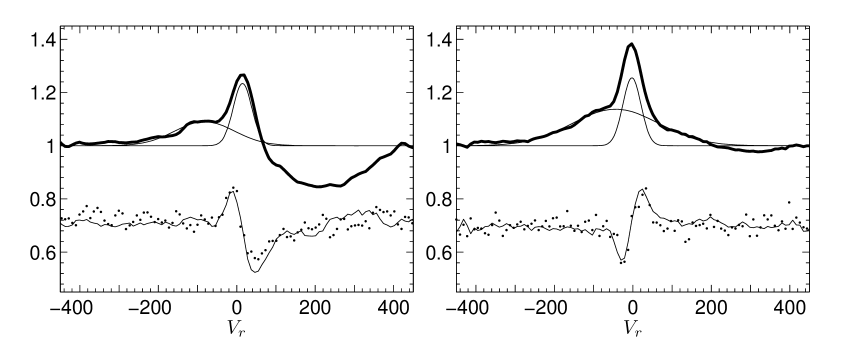
Figure 1: Stokes $I$ and $V$ profiles of He I 5876 line for JD 2453748.30 (left panel) and JD 2453784.29 (right panel). Solid bold line represents $I$-profile normalized to the continuum level. Solid thin lines are Gaussians which correspond to a narrow and a broad components. Dots represents observed Stokes $V$-profile on which model $V$-profile was overplotted by a solid thin line. Both $V$-profiles were multiplied by 10 times and shifted to 0.7 for readability. An abscissa is the velocity in km s^-1 from the line center $\lambda_{0}=5875.6$ Å.

For illustrative purposes we computed model $V$-profiles. After the field and corresponding shift $\Delta\lambda_{rl}$ between right- and left polarized profiles had been derived, we computed the difference between two $I$-profiles, the first of them was shifted by $\Delta\lambda_{rl}/2$ to the left and the second was shifted by the same amount to the right. Having divided the difference by $I(\lambda)$, we simulated a model $V$-profile. It can be seen that in an emission part of the $I$-profile the model $V$-profile well approximates observed one and clearly indicates that the field in observations presented on the left and right panels of Fig. 1 has the opposite sign.

Also we have detected twice (JD 2453748.30 and 2453749.33) at $>3\sigma$-level $B_{z}$ in Na I D line formation region – see Table 3. Lande factor for both lines of the doublet was assumed to be equal $1.33$ (Frish, 2010). The Stokes $I$ and $V$ profiles for Na I D lines at the mentioned moments are shown on Fig. 2. Model $V$-profile for Na I D lines was computed in the same manner as for He I 5876 Å  line.

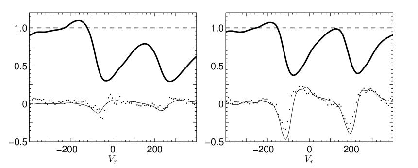
Figure 2: The same as in Fig. 1, but for Na I D doublet lines. The left panel corresponds to the moment JD 2453748.30 and the right panel to JD 2453749.33. In contrast to the previous figure observational and model $V$-curves, although were multiplied by 10 times, but were not shifted along ordinate axis. In addition the spectrum of a veiled photosphere was not removed on this figure. Zero point of abscissa axis corresponds to the center of D₂ line $(\lambda=5889.95$ Å).

In the conclusion of this section note the following. It can be found from table 1 of Petrov et al. (2001) paper that RW Aur’s radial velocity of photospheric lines averaged over all obsrvations with $\sigma^{-2}$ weight is equal to $+16.0$ km s^-1. The same quantity derived from our observations is equal to $+10.5$ km s^-1. Possible reasons of the discrepancy will be discussed in the Conclusion.

Magnetic field in the hotspots

As was noted in the Introduction some lines in RW Aur’s spectrum have redshifted absorption feature extended up to the velocity $\simeq 400$ km s^-1 (see e.g. the left panel of Fig. 1) indicating matter infall with the same velocity. Accreted gas should be deccelerated near stellar surface in the shock and abruptly heated up at the shock front to $T\sim 10^{6}\,K.$ Post shock zone is the region were thermal and kinetic energy of accreted matter is radiated away in X-ray and far UV bands so gas cools down, deccelerates and finally gradually settles to the stellar surface. The source of an emission continuum are regions at the footstep of accretion streams, which absorb the hard radiation of the shock and re-emit it mainly in the region from 0.3 to 1 $\mu.$ These regions are used to call hotspots although their temperature is $<9000$ K (Lamzin, 1995; Calvet & Gullbring, 1998).

It was found about 20 years ago that many emission lines in CTTS’s spectra are superposition of so-called narrow and broad components which probably formed in regions with different physical conditions – see e.g. Batalha et al. (1996) and references therein. In the case of RW Aur lines of ionized metals and He I have two-component structure, He II 4686 has no broad component and vice versa hydrogen lines and other neutrals have no significant narrow component (Petrov et al., 2001).

Fig. 1) demonstrates how emission part of He I 5876 line’s $I$-profile can be decomposed onto two Gaussians, which correspond to narrow and broad components. As was mentioned in the Introduction Petrov et al. (2001) have found that radial velocity of the narrow component $V_{r}^{NC}$ varied with a period of about 2.77 days around a mean velocity $\simeq+10$ km s^-1 with an amplitude $\simeq 15$ km s^-1.

Petrov et al. (2001) suggested that narrow components are formed in the hotspot(s) i.e. at the stellar surface. But it would be more precisely to say that they are formed above the photosphere of the hotspot, i.e. in the post shock cooling zone where helium atoms and first ions of metals appear due to recombination from higher ionization states. This remark helps to explain in natural way why narrow components have small positive velocity relative to the photosphere. It becames also clear why radial velocity of He II 4686 line is greater than $V_{r}^{NC}$ of He I 5876 line (Petrov et al., 2001): He⁺ ions appears behind the shock front before helium atoms and thus have greater velocities.

However in the case of RW Aur the accretion shock is placed very close to the stellar surface. Indeed an existence of a veiling continuum with a flux at $\lambda=5500$ Å  exceeding the photospheric one by 2-3 times (Petrov et al., 2001) suggests that pre-shock gas density is greater than $10^{11}$ sm${}^{-3}.$ Hence, a distance between the shock front and the stellar photosphere is much smaller than the stellar radius (Lamzin, 1995) what means that narrow components are formed practically at the stellar surface.

It can be seen from the comparison of observed $I$-profile and modeled $V$-profile on Fig. 1 that the difference $F_{\lambda}^{r}-F_{\lambda}^{l}$ is maximal where $I$-profile has a steep gradient. Therefore the shape of an observed $V$-profile of He I 5876 does not constrain a region of the strong $B_{z}$ by only a formation region of the narrow component. We found that if to assume a priori (i.e. before cross corellation procedure) that $B_{z}=0$ in the broad component then then field averaged over the narrow component increases by no more than 1 $\sigma_{B}$.

There is no doubt that the field changes its polarity. In the frame of magnetospheric accretion model this fact can be naturally explained by a change of an orientation of the hotspot relative to the Earth due to stellar axial rotation. It means that the variations of the field should be periodical with the period of the stellar axial rotation.

On Fig. 3 phase curves of observed $B_{z}$ derived over the He I 5876 line are shown for the period of 2.77 days. Our observations cover a time span of a few years and during the time a geometry and strength of the field could change: Donati et al. (2008) have discovered such changes for CTTS BP Tau by a comparison of stellar magnetogramms obtained with a time span of 10 month.

To minimize the effect of a physical variability of the field, we considered separately two sets of observations from Table 2, which contain 5 observations (in Table the sets are separated by a horizontal line). The first set (left panel) contains observations, which were carried out during 40 days and the second set (right panel) – the next five observations covered a time span of 26 days. A global changing of a magnetic structure over times less than 40 days seems unlikely, therefore the observational variations of the magnetic field during each set is caused by the axial rotation. What about the last observation, it was carried out 360 days after tenth observation and does not shown on Fig. 3.

Figure 3: A phase curve of variations of $B_{z}$ (kG) in a region of the He I 5876 line formation for $P=2.77$ days. Numeration of the dots on the figure corresponds to the numeration of spectra in Table 2. An ordinate is the field in kG. $\varphi=0$ phase corresponds to the dot # 1 on a right panel and to the dot # 6 on a left panel.

The figure suggests that in the first set $B_{z}$ changes from $+1.1\pm 0.15$ kG to $-1.47\pm 0.15$ kG during $\simeq 15$ minutes (the time, which correspond to a phase difference of the dots 4 and 2). In the second set nearly the same changing of the field strength occurred during a time span of $<50$ minutes (the dots 8 and 10), and the field recovered to an initial level after $<3$ hours (the dot 9). Such kind of variations cannot be explained by only an orbital motion of the star with $P\simeq 2.77$ due to an existence of a close companion. We found that the same statement is valid for any period in the range from 2.5 to 2.9 days that includes all possible values of a ”short”  $(\sim 2.7^{d})$ period for RW Aur A (Petrov et al., 2001).

One the other hand, we have found that for a number of values $P$ in the range from 5.5 to 5.7 days a smooth dependence $B_{z}=B_{z}(\varphi)$ could be obtained even without a phase shift between the sets. An example of such curve is shown on Fig. 4 for $P=5.576^{d}$ but similar smooth curve turns out for $P=5.6659^{d}.$ In other words for $P\sim 5.6$ days observed variability of $B_{z}$ can be explained as the result of rotational modulation only, i.e. assuming that geometry and field strength in the accretion zone did not change significantly during three years of the observations.

Figure 4: Phase curve of variations of $B_{z}$ (kG) with $P=5.576^{d}$ for He I 5876 line (triangles) and for Na D doublet lines (open circles).

Having only 11 measurements of $B_{z}$ we cannot derive a certain period of the axial rotation of RW Aur A as well as make a conclusion concerning a variability of a geometry and/or physical conditions in the accretion zone from January 2006 to January 2009. However, we can certainly argue that our results contradict to the rotational period $\simeq 2.77^{d},$ but well consist with $P\simeq 5.6^{d},$ which corresponds to the model of two hotspots with opposite polarities of the field and located in opposite hemispheres.

In the frame of the model observed peculiarities of RW Aur A spectrum can be explained in the following way (Petrov et al., 2001). Temperature increases with height above hotspot’s photosphere what results in appearence of emission lines. The strongest lines appear in the spectrum as the narrow components of helium and ionized metals lines, but more faint lines blend absorption lines of the photosphere to some extent. The hotspots move relative to the Earth due to stellar rotation. Due to this reason radial velocities of narrow components $V_{r}^{NC}$ vary as well as a center of gravity of the photospheric lines what looks like a variation of their radial velocity $V_{r}^{ph}.$ This effect explains why $V_{r}^{NC}$ and $V_{r}^{ph}$ vary in the antiphase.

It can be explained in the same way why a phase curve of He I 5876 line’s narrow component equivalent width $EW_{NC}$ is shifted by one fourth of the rotational period relative to $V_{r}^{NC}(\varphi)$ curve. Indeed when the center of each spot crosses the plane formed by the Earth and stellar rotational axis (the central meridian), $V_{r}^{NC}\simeq 0$ and observed area of the spot and therefore $EW_{NC}$ have maximum values. After 1/4 of the period the spot center is close to a limb and modulus of $V_{r}^{NC}$ has a maximum but $EW_{NC}$ has a minimum.

Our data are insufficient to reconstruct a magnetic map of the star, so we will give below only semi-qualitative constraints on a geometry and parameters of accretion zones.

A relation between $B_{z}$ measured over the He I 5876 line and an equivalent width of the narrow component of the line is shown on Fig. 5. Bear in mind written above it follows from the figure that maximal values of $\mid B_{z}\mid$ is reached when the hotspots cross the central meridian and are close to zero when hotspots are near stellar limb. One can conclude therefore that magnetic field lines in the spots make large angle relative to stellar surface, what means that toroidal component of the field in the spots is much less than poloidal one.

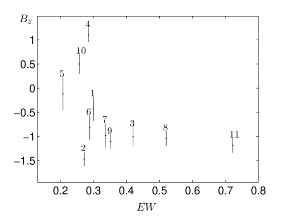
Figure 5: A dependence of $B_{z}$ modulus (kG) on equivalent width of the narrow component of the He I 5876 line (Å).

It can be seen from Fig. 1 that when $B_{z}$ has large negative value (the left panel) the helium line demonstrates deep redshifted absorption feature which has velocity extention up to $+400$ km s^-1 and vice versa in the case of large positive field (the right panel) we observe shallow absorption. It is a particular case of the general trend: when the field increases from negative to positive values, the equivalent width of red absorption decreases. It can be seen more clear if to use equivalent width of the far redshifted part of the profile and additionaly subtract veiled photosphere – see Fig. 6. Note that the main uncertainty in $EW_{RA}$ is due to uncertainty in veiling determination.

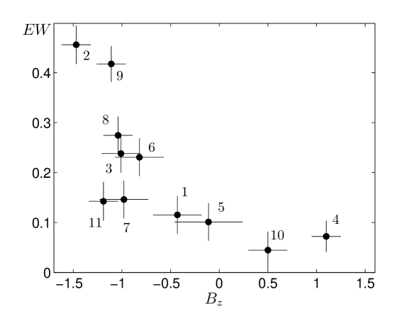
Figure 6: A dependence of equivalent width of absorption feature (Å) of the He I 5876 line derived in the range from $+200$ to $+400$ km s^-1 on the field $B_{z}$ (kG).

Because negative values of $B_{z}$ appear more frequently than positive $B_{z}$, we conclude that a spot with $B_{z}<0$ is located in a hemisphere above a midplane of an accretion disc relative to the Earth (the ”upper” spot) and a spot with $B_{z}>0$ is below the disc (the ”low” spot). One can conclude that longitudes of the upper and low spots differ by $\simeq 180^{o}$ because variations of photospheric lines radial velocities are well convolved with period $\simeq 2.77^{d}\simeq P/2.$ The lower spot can be observed from the Earth if its stellar latitude $\theta<i,$ where $i\simeq 65^{o}$ is the inclination of the stellar rotational axis to the line of sight (see the end of this section).

Maximal (absolute) values of field $\left|B_{z}\right|$ we observed in the upper and low spots differ from each other 1.5-2 times. If spots have nearly identical parameters then the same ratio must take place for averaged cosines of angles between the field lines and the line of sight for moments when the spots cross the central meridian. It follows from the modelling we carried out (assuming the field of the star is dipol and intensity in the He I 5876 line is nearly isotropic) that such cosine ratio could be obtained if spots located at latitudes $30^{o}<\theta<50^{o}.$

Red wing absorption of the helium line is formed in accreted gas of pre-shock zone. It can be easily seen that when the upper spot is visible from the Earth accretion stream is projected onto larger area of stellar surface than in the case when we observe low spot. We suppose that just due to this reason $EW_{RA}$ is much less when upper spot crosses the central meridian than in the case when low spot passes throug the same meridian.

As was noted before in the case of RW Aur A accretion shock front is located very close to stellar surface. Therefore pre-shock zone is always projected onto underlying hotspot. Apparently it is the reason why $EW_{RA}$ has never reached zero. It is interesting to note that absorption feature in the red wing of the He I 5876, Na I 5898 as well as O I 7773 lines (Petrov et al., 2001) extends up to +400 km s^-1 in all spectra that we know. In other words at any position of the spots relative to the Earth we observe the constant red cutoff velocity of the red wing. It can be explained by assuming that $V_{m}=400$ is the largest velocity of the accreting gas and the field lines come out of the spots in a broad interval of angles.

If the mass of RW Aur A $M_{*}\simeq 1.3\,M_{\odot}$ (White & Ghez, 2001) then corotation radius for rotational period $P\simeq 5.6$ is:

$$R_{c}={\left({GM_{*}P^{2}\over 4\pi^{2}}\right)}^{1/3}\simeq 14.5\,R_{\odot}\simeq 7.6\,R_{*},$$

where $R_{*}\simeq 1.9\,R_{\odot}$ is the stellar radius (see the end of this section). As far as matter can not freez into magnetic field lines at distance $r>R_{c}$ free-fall velocity at the stellar surface is smaller than $V_{u}$ value defined by equation:

$${GM_{*}\over R_{*}}-{GM_{*}\over R_{c}}={V_{u}^{2}\over 2},$$

what means that $V_{u}\simeq 480$ km s^-1.

If to replace $V_{u}$ by $V_{m}$ then it follows from the same equation that gas should start to fall along magnetic field lines from distance $R_{f}\simeq 2.6\,R_{*}\simeq 4.9\,R_{\odot}$ to reach stellar surface with velocity 400 km s^-1.

Let us discuss in brief the question about the value of angle between rotational axis of RW Aur A and the line of sight. Hirth et al. (1994) have discovered a bipolar jet of RW Aur. Studying temporal variations of the jet structure López-Martín et al. (2003) have found that the angle between the jet and the line of sight is $i=46^{o}\pm 3^{o}.$ Cabrit et al. (2006) have found discs around both components of RW Aur and concluded that the jet is oriented along circumprimary rotational axis of RW Aur A disk, such as $i$ found by López-Martín is a lower limit and in fact $45^{o}<i<60^{o}.$ If the rotational axes of the disc and the star are aligned, then the inclination of RW Aur A also must be bounded between $45^{o}$ and $60^{o}.$ Similar estimate was derived by Alencar et al. (2005) in modeling hydrogen and Na D line profiles in the frame of disc wind model: $55^{o}<i<65^{o}.$

Petrov & Kozack (2007) have argued that irregular light variability of RW Aur A is mostly associated with eclipses by dust clouds. Taking into account existed estimate $i\simeq 45^{o}$ of López-Martín et al. (2003) Petrov & Kozack supposed that the dust clouds are formed in the disc wind, because the star could not be occulted by the disc itself at such inclination. However as far as $i=45^{o}$ is turned out to be a lower limit one can suppose that the dust clouds are inhomogeneities in the disc and then at least internal regions of the disc shoul be inclined to the line of sight by an angle significantly greater than $45^{o}.$

Note finally that observed value $v_{e}\sin i=17.2\pm 1.5$ km s^-1 (Hartmann & Stauffer, 1989). If RW Aur A’s rotational period is $P\simeq 5.6$ days then $R_{*}\sin i\simeq 1.9\pm 0.2$ $R_{\odot}$ what can be consistent with the estimate of the stellar radius $R_{*}=1.7\pm 0.3$ $R_{\odot}$ (White & Ghez, 2001) within uncertainties only at large $i.$ Taking in to account all these arguments we regard as reasonable estimates $i\approx 65^{o},$ $R_{*}\simeq 1.9$ $R_{\odot}.$

A magnetic field at an outer boundary of a magnetosphere and in a wind

As follows from Tabl. 2 and 3 $B_{z}$-values did not differ always from zero within errors of measurements in formation region of iron lines, which have only broad component. The example of JD 2453784 night (when we found $B_{z}=+1.10\pm 0.15$ kG in He I 5876 line formation region but $B_{z}=-0.09\pm 0.20$ kG over Fe II lines) clearly demonstrates that magnetic field strength is different in formation regions of narrow and broad components of emission lines. Another example is JD 2454846 night when $B_{Z}$ in the broad component was $-0.11\pm 0.10$ kG but $-1.19\pm 0.15$ kG in He I narrow component. Thus our data confirm the viewpoint according to which narrow and broad components are formed in different regions.

Gómez de Castro & Verdugo (2003) argued that broad components are formed at outer boundary of stellar magnetosphere within an internal ring-like region of the disk. A half-width of the broad components in RW Aur spectra, except for H_α-line, is $\simeq 200$ km s^-1 at continuum level $\simeq 200$ km s^-1 what consists with a projection of orbital (keplerian) velocity to the line of sight at distance $R_{f}\simeq 2.6\,R_{*}$ from the star:

$$V_{K}=\sqrt{{GM\over R_{f}}}\,\sin i.$$

Remind that $R_{f}$ is the distance from which free-falling gas reaches velocity about 400 km s^-1 at the surface of the star.

Another nontrivial result of our observations is detection of magnetic field in the formation region of Na I D lines in two spectra out of 11. The detection is out of doubts in these two cases: firstly $B_{z}$ differs from zero at more than $3\,\sigma$ (see Table 2) and secondly $V$-curves have similar shapes for both lines of the doublet – see Fig. 2. It is very important to note that field strength up to $\simeq 0.8$ kG was found in the region where line’s profile from $\simeq-180$ to 0 km s^-1 is formed, i.e. in the outflow.

Existence of sodium atoms in the wind indicates that gas temperature in the outflow is relatively low $(T<10^{4}$ K) while gas moves with velocities up to $V_{w}\sim 200$ km s^-1 what follows from an extension of Na I D₂ line’s blue wing. Thus $V_{w}$ is more than one order of magnitude greater than local sound velocity, what means that the outflow is driven by nonthermal, probably magneto-rotational mechanism, and the outflow is launched from the disc rather than from stellar surface (Cabrit, 2007; Matt & Pudritz, 2007).

According to Table 2 magnetic field strength variations occurred in the following way during the first three nights of our observations. At the first night $B_{z}$ in the spots and in the wind was zero at $3\,\sigma$-level. Two days later $B_{z}$ has reached its maximum value $-1.45\pm 0.15$ kG in the upper spot and was equal to $-0.18\pm 0.05$ kG in the wind. At the next night $B_{z}$ has decreased to $-1.01\pm 0.20$ kG in the upper spot but increased up to $-0.81\pm 0.08$ kG in the wind.

Bear in mind discussion in the previous Section this sequence of events can be interpreted in the following way. At the first night the upper spot was located near stellar limb and then $B_{z}$ in the wind was zero. Two days later when the spot has passed through the central meridian wind’s field became noticeble and reached its maximal value one day later. Note that this conclusion (sequence of events) does not depend on precise (unknown) value of stellar rotation period $P.$ But if $P$ indeed equal to $5.576^{d}$ then it follows from phase curve shown on Fig.4 that the longitude component of wind’s magnetic field has detectable strength only at certain orientation of the system relative to the observer, reaching its maximum value at approximately $1/4$ of rotation period after passage of upper spot throug the central meridian. Of course it is true only if the discovered field is related with (quasi)stationary gas outflow rather than a fortuitous gas ejection.

To explain observed profiles of H${}_{\beta},$ H_γ and Na I D lines that are originated in RW Aur outflow Alencar et al., (2005) suggested phenomenological model of the disc wind which is launched from narrow $(\Delta r/r\ll 1)$ region near inner boundary of accretion disc. As far as the aim of these authors was to reproduce time-averaged line profiles they considered axisymmetric outflow and achieved reasonable agreement with observations.

Similar picture of the outflow has been reproduced by Romanova et al. (2009) in numerical MHD simulations. It turned out that in an axisymmetric case, when stellar rotational axis coincides with magnetic dipole axis, the outflow is launched from narrow region at the boundary between the disc and stellar magnetosphere and forms thin-walled cone with a cone half-angle $\simeq 30^{o}-40^{o}$ (so called conical wind). Test simulations for non-axisymmetric case, when the angle between rotational and magnetic axes was $30^{o},$ have shown that the outflow in the cone occurred as before from the internal boundary of the disc and with the same cone angle but with azimuthal inhomogeneities of gas parameters. It can be said that in the wind (above and below the disc) a spiral stream is formed. Inside the stream gas density and field strength are higher than in the rest part of the outflow.

This picture is in a qualitative agreement with observations of RW Aur: firstly, blueshifted absorption Na D₂ line is present permanently (Alencar et al., 2005), secondly, a non-zero field $B_{z}$ was observed only when the upper spot was near the central meridian.

At the first glance it seems that observed value $B_{z}\simeq 0.8$ kG is too strong for a wind because for the magnetic field strength about 2 kG at the stellar surface the field strength at $r\simeq 2.6$ $R_{*}$ should be $\sim 0.1$ kG. However in the model of conical wind the disc compresses stellar magnetosphere what should increase the field strengs at the base of the stream.

Conclusion

We obtained 18 measurements of RW Aur A average magnetic field’s longitudinal component between 2006 and 2009 yrs. Our data scaterred in time and can not be used for Zeeman imaging but a number of nontrivial conclusions were obtained.

First of all one can definitely state that results of our observations contradict to hypothesis that explains periodical variations of RW Aur A photospheric line’s radial velocity as the result of orbital motion with a period of $\simeq 2.77^{d}.$ At the same time our data consist with Petrov et.al (2001) model of two hotspots with opposite magnetic field polarities that located in opposite hemispheres, such as stellar axial rotational period $P\simeq 5.6^{d}.$

Our data are insufficient to derive precise period but we found that for $P=5.576^{d}$ and $P=5.6659^{d}$ $B_{z}$-phase curves have the following features:

1) maximum and minimum values of $B_{z}$ in the spots are shifted in phase by $\simeq 0.5$ what is expected in the case of two spots with longitude difference near $180^{o};$

2) longitudinal component of magnetic field in RW Aur A’s wind becomes significant within a certain interval of the phase curve, i.e. at a certain orientation of the system relative to the Earth, reaching the maximum nearly 1/4 of the period after the passage of upper spot throug the central meridian. It can be considered as an argument that discovered magnetic field in the wind is related with a (quasi)stationary outflow rather than sporadic gas ejection.

We found that average value of RW Aur A’s photospheric lines radial velocity $V_{r}^{ph}$ is smaller by 5 km s^-1 than value found by Petrov et al. (2001). This discrepancy is seemed to be significant because the amplitude of $V_{r}^{ph}$ variations due to stellar rotation is $\simeq 6$ km s${}^{-1}.$ We have found two papers which contains results of more old measurements of RW Aur’s $V_{r}^{ph}$ measurements: the paper of Herbig (1977), which contains only one measurement, and the paper of Hartmann et al. (1986), which includes 13 measurements close in time. All available data are shown on Fig. 7. Parabola was drawn throught average values of Hartmann et al., Petrov et.al and our data (dashed line).

Figure 7: Variations of radial velocities of RW Aur photospheric lines. Single measurement of Herbig (1977) is depicted by filled circle and measurements of Hartmann et al. (1986), Petrov et al. (2001) and our data are shown with open circles, triangles and squares respectively. The dashed line is drawn through average values of each subset.

The measurements presented on the figure are insufficient for an unambiguous conclusion about secular variations of RW Aur’s radial velocity and additional observations are necessary. However one can conclude that variations of $V_{r}^{ph}$ by a few km s^-1 during $\sim 10$ years cannot be explained by RW Aur B that located at a distance more than 100 a.u. from the primary. Thus we return again, but on different grounds than Petrov et al. (2001), to a possibility that RW Aur is a triple system with orbital period of hypothetic RW Aur C of several decades.

We thank S. Alencar and P. P. Petrov for the spectra provided to us as well as D. O. Kudryavtsev and D. A. Smirnov for the help with observations.

References

- [1] Alencar S. H. P., Basri G., Hartmann L., Calvet N., Astron. Astrophys. 440, 595 (2005).
- [2] [0.3cm]
- [3] Babcock H. W., Astrophys. J. Suppl. Ser. 3, 141 (1958).
- [4] [0.3cm]
- [5] Bagnulo S., Jehin E., Ledoux C. et al., ESO Messenger 114, 10 (2003).
- [6] [0.3cm]
- [7] Batalha C. C., Stout-Batalha N. M., Basri G., Nerra M. A. O., Astrophys. J. Suppl. Ser. 103, 211 (1996).
- [8] [0.3cm]
- [9] Bertout C., Ann. Rev. Astron. Astrophys. 27, 351 (1989).
- [10] [0.3cm]
- [11] Cabrit S., Pety J., Pesenti N., Dougados C., Astron. Astrophys. 452, 897 (2006).
- [12] [0.3cm]
- [13] Cabrit S., ”Star-Disk Interaction in Young Stars” Proc. IAU Symp. 243, 2007 J. Bouvier & I. Appenzeller, eds., p.203 (2007)
- [14] [0.3cm]
- [15] Calvet N., Gullbring E., Astrophys. J. 509, 802 (1998).
- [16] [0.3cm]
- [17] Chountonov G. A., Magnetic stars: Proc.of the Intern.Conf., N.Arkhyz, Eds. Yu. V. Glagolevskij, D. O. Kudryavtsev, I. I. Romanyuk, Moscow, p.286 (2004).
- [18] [0.3cm]
- [19] Chountonov G. A., Smirnov D. A., Lamzin S. A., Astronomy Letters 33, 38 (2007).
- [20] [0.3cm]
- [21] Donati J.-F., Jardine M. M., Gregory S. G. et al., MNRAS 386, 1234 (2008).
- [22] [0.3cm]
- [23] Donati J.-F., Landstreet J. D., Ann. Rev. Astron. Astrophys. 47, 333 (2009).
- [24] [0.3cm]
- [25] Frish S. E., ”Optical spectra of atoms” (in Russian), SPb., ”Lan” (2010).
- [26] [0.3cm]
- [27] Gómez de Castro A. I., Verdugo E., Astrophys. J. 597, 443 (2003).
- [28] [0.3cm]
- [29] Hartigan P., Hartmann L., Kenyon S. et al., Astrophys. J. Suppl. Ser. 70, 899 (1989).
- [30] [0.3cm]
- [31] Hartmann L., Hewett R., Stahler R., Matheiu R. D., Astrophys. J. 309, 275 (1986).
- [32] [0.3cm]
- [33] Hartmann L., Stauffer J. R., Astron. J. 97, 873 (1989).
- [34] [0.3cm]
- [35] Herbig G. H., Astrophys. J. 214, 747 (1977).
- [36] [0.3cm]
- [37] Hill G. M., Bohlender D. A., Landstreet J. D. et al., MNRAS 297, 236 (1998).
- [38] [0.3cm]
- [39] Hirth G. A., Mundt R., Solf J., Ray T. P., Astrophys. J. 427, L99 (1994).
- [40] [0.3cm]
- [41] Johnstone R. M., Penston M. V., MNRAS 219, 687 (1986).
- [42] [0.3cm]
- [43] Joy A. H., van Biesbroeck G., Publ. Astron. Soc. Pacific 56, 123 (1944).
- [44] [0.3cm]
- [45] Joy A. H., Astrophys. J. 102, 168 (1945).
- [46] [0.3cm]
- [47] Kupka F., Piskunov N., Ryabchikova T. A. et al., Astron. Astrophys. Suppl. Ser. 138, 119 (1999).
- [48] [0.3cm]
- [49] Lamzin S. A., Astron. Astrophys. 295, L20 (1995).
- [50] [0.3cm]
- [51] López-Martín L., Cabrit S., Dougados C., Astron. Astrophys. 405, L1 (2003).
- [52] [0.3cm]
- [53] Matt S., Pudritz R. E., ”Star-Disk Interaction in Young Stars” Proc. IAU Symp. 243, 2007 J. Bouvier & I. Appenzeller , eds., p.299 (2007).
- [54] [0.3cm]
- [55] Panchuk V. E., Preprint SAO RAS N 154 (2001)
- [56] [0.3cm]
- [57] Petrov P. P., Gahm G. F., Gameiro J. F. et al.,Astron. Astrophys. 369, 993 (2001).
- [58] [0.3cm]
- [59] Petrov P. P., Kozack B. S., Astron. Rep. 51, 500 (2007).
- [60] [0.3cm]
- [61] Romanova M. M., Ustyugova G. V., Koldoba A. V. et al., Astrophys. J. 595, 1009 (2003).
- [62] [0.3cm]
- [63] Romanova M. M., Ustyugova G. V., Koldoba A. V., Lovelace R. V. E., MNRAS 399, 1802 (2009).
- [64] [0.3cm]
- [65] Symington N. H., Harries T. J., Kurosawa R., MNRAS 356, 1489 (2005).
- [66] [0.3cm]
- [67] White R. J., Ghez A. M., Astrophys. J. 556, 265 (2001).